From Drivers to Athletes – Modeling and Simulating Cross-Country Sking Marathons

Abstract

Traffic flow of athletes in classic-style cross-country ski marathons, with the Swedish Vasaloppet as prominent example, represents a non-vehicular system of driven particles with many properties of vehicular traffic flow such as unidirectional movement, the existence of lanes, and, moreover, severe traffic jams. We propose a microscopic acceleration and track-changing model taking into account different fitness levels, gradients, and interactions between the athletes in all traffic situations. The model is calibrated on microscopic data of the Vasaloppet 2012 Using the multi-model open-source simulator MovSim.org, we simulate all 15 000 participants of the Vasaloppet during the first ten kilometers.

1 Introduction

Traffic jams are not only observed in vehicular traffic but also in the crowd dynamics of mass-sport events, particularly cross-country ski marathons. The Swedish Vasaloppet, a 90-km race with about 15 000 participants, is the most prominent example (cf. Fig. 1). Several other races attract up to 10 000 participants. Consequently, “traffic jams” among the athletes occur regularly. They are not only a hassle for the athletes but also pose organisational or even safety threats. While there are a few scientific investigations of the traffic around such events ahmadi2011analysis , we are not aware of any investigations on the crowd dynamics of the skiers themselves.

Unlike the athletes in running or skating events TGF13-running , the skiers in Marathons for the classic style (which is required in the Vasaloppet main race) move along fixed tracks, i.e., the traffic flow is not only unidirectional but lane based. This allows us to generalize car-following and lane changing models TreiberKesting-Book to formulate a microscopic model for the motion of skiers.

Simulating the model allows event managers to improve the race organization by identifying (and possibly eliminating) bottlenecks, determining the optimum number of starting groups and the maximum size of each group, or optimizing the starting schedule TGF13-running .

We propose a microscopic acceleration and track-changing model for cross-country skiers taking into account different fitness levels, gradients, and interactions between the athletes in all traffic situations. After calibrating the model on microscopic data of jam free sections of the Vasaloppet 2012, we apply the open-source simulator MovSim.org movsim to simulate all 15 000 participants of the Vasaloppet during the first ten kilometers. The simulations show that the initial jam causes a delay of up to 40 minutes which agrees with evidence from the data.

The next section introduces the model. In Section 3, we describe the calibration, the simulation, and the results. Section 4 concludes with a discussion.

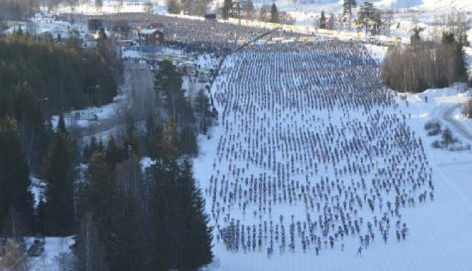
Figure 1: Starting phase of the Vasaloppet 2012.

2 The Model

Unlike the normal case in motorized traffic, the “desired” speed (and acceleration) of a skier is restricted essentially by his or her performance (maximum mechanical power $P=P_{\rm max}$), and by the maximum speed $v_{c}$ for active propulsion ($P=0$ for $v\geq v_{c}$). Since, additionally, $P\to 0$ for $v\to 0$, it is plausible to model the usable power as a function of the speed as a parabola,

$$P(v,v_{c})=4P_{\rm max}\frac{v}{v_{c}}\left(1-\frac{v}{v_{c}}\right)\theta(v_{c}-v),$$ (1)

where $\theta(x)=1$ if $x\geq 0$, and zero, otherwise. While the maximum mechanical power is reached at $v_{c}/2$, the maximum propulsion force $F_{\rm max}=4P_{\rm max}/v_{c}$, and the maximum acceleration

$$a_{\rm max}=\frac{4P_{\rm max}}{mv_{c}},$$ (2)

is reached at zero speed. The above formulas are valid for conventional techniques such as the “diagonal step” or “double poling”. However, if the uphill gradient (in radian) exceeds the angle $\alpha_{\rm slip}=a_{\rm max}/g$ (where $g=9.81\,\mathrm{m/s^{2}}$), no forward movement is possible in this way. Instead, when $\alpha>\alpha_{\rm max}/2$, athletes use the slow but steady “fishbone” style described by (1) with a lower maximum speed $V_{c2}$ corresponding to a higher maximum gradient $4P_{\rm max}/(gmv_{c_{2}})$. In summary, the propulsion force reads

$$F(v,\alpha)=\left\{\begin{array}[]{ll}P(v,v_{c})/v&\alpha<\alpha_{\rm max}/2\\ P(v,v_{c2})/v&{\mbox{ otherwise.}}\end{array}\right.$$ (3)

Balancing this force with the inertial, friction, air-drag, and gravitational forces defines the free-flow acceleration $\dot{v}_{\rm free}$:

$$m\dot{v}_{\rm free}=F(v)-\frac{1}{2}c_{d}A\rho v^{2}-mg(\mu_{0}+\alpha).$$ (4)

If the considered skier is following a leading athlete (speed $v_{l}$) at a spatial gap $s$, the free-flow acceleration is complemented by the decelerating interaction force of the intelligent-driver model (IDM)TreiberKesting-Book leading to the full longitudinal model

$$\frac{{\rm d}v}{{\rm d}t}={\mbox{ min}}\left\{\dot{v}_{\rm free},\,a_{\rm max}\left[1-\left(\frac{s^{*}(v,v_{l})}{s}\right)^{2}\right]\right\},$$ (5)

where the desired dynamical gap of the IDM depends on the gap $s$ and the leading speed $v_{l}$ according to

$$s^{*}(v,v_{l})=s_{0}+\max\left(0,\,vT+\frac{v(v_{l}-v)}{2\sqrt{a_{\rm max}b}}\right).$$ (6)

Besides the ski length, this model has the parameters $c_{d}A\rho/m$, $\mu_{0}$, $P_{\rm max}/m$, $v_{c}$ (defining $a_{\rm max}$), $v_{c2}$, $s_{0}$, $T$, and $b$ (see Table 1). It is calibrated such that the maximum unobstructed speed $v_{\rm max}$ on level terrain, defined by $F(v_{\rm max},0)-c_{d}A\rho v_{\rm max}^{2}/2-mg\mu_{0}=0$, satisfies the observed speed distributions on level unobstructed sections (Fig. 2).

2.1 Lane-changing model

We apply the general-purpose lane−changing model MOBIL TreiberKesting-Book . Generally, lane changing and overtaking is allowed on either side and crashes are much less avoided than in vehicular traffic, so, the symmetric variant of the model with zero politeness and rather aggressive safety settings is appropriate. Lane changing takes place if it is both safe and advantageous. The safety criterion is satisfied if, as a consequence of the change, the back skier on the new track is not forced to decelerate by more than his or her normal deceleration ability $b$:

$$\frac{{\rm d}v_{\rm back,new}}{{\rm d}t}\geq-b.$$ (7)

A change is advantageous if, on the new track, the athlete can accelerate more (or needs to decelerate less) than on the old track:

$$\frac{{\rm d}v_{\rm front,new}}{{\rm d}t}\geq\frac{{\rm d}v_{\rm actual}}{{\rm d}t}+\Delta a,$$ (8)

where the only new parameter $\Delta a$ represents some small threshold to avoid lane changing for marginal advantages. Note that for mandatory lane changes (e.g., when a track ends), only the safety criterion (7) must be satisfied.

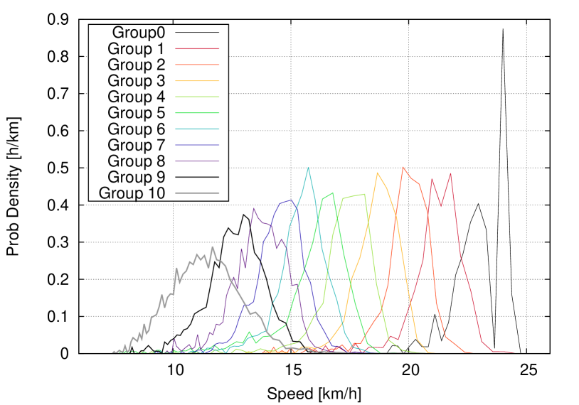
Figure 2: Speed density functions for the section between Station 1 and 2 for each starting group. No jams were observed in this section.

Table 1: Model parameters of the proposed longitudinal model

Parameter	Typical Value ($4^{\rm th}$ starting group)
ski length $l$	2 m
Mass $m$ incl. equipment	80 kg
air-drag coefficient $c_{d}$	0.7
frontal cross section $A$	$1\,\mathrm{m^{2}}$
friction coefficient $\mu_{0}$	0.02
maximum mechanical power $P_{\rm max}$	150 W
limit speed for active action $v_{c}$	6 m/s
time gap $T$	0.3 s
minimum spatial gap $s_{0}$	0.3 m
normal braking deceleration $b$	$1\,\mathrm{m/s^{2}}$
maximum deceleration $b_{\rm max}$	$2\,\mathrm{m/s^{2}}$

3 Simulation Results

We have simulated all of the 15 000 athletes of the Vasaloppet 2012 for the first 10 km (cf. Fig. 3) by implementing the model into the open-source traffic simulator MovSim.org. The starting field includes 70 parallel tracks (cf. Fig. 1) where the 10 starting groups (plus a small elite group) are arranged in order. Further ahead, the number of tracks decreases gradually down to 8 tracks at the end of the uphill section for $x\geq 7\,\mathrm{km}$. The uphill gradients and the course geometry (cf. Fig. 3) were obtained using Google Earth.

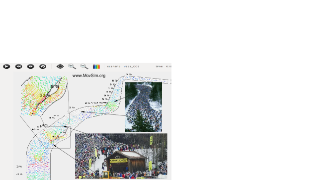
Figure 3: Screenshot of the MovSim Simulation of the first 10 km of the Vasaloppet 2012 (center) with an enlargement of the diverge-merge section (left top). Also shown are two photos of the crowd flow at the corresponding sections (right).

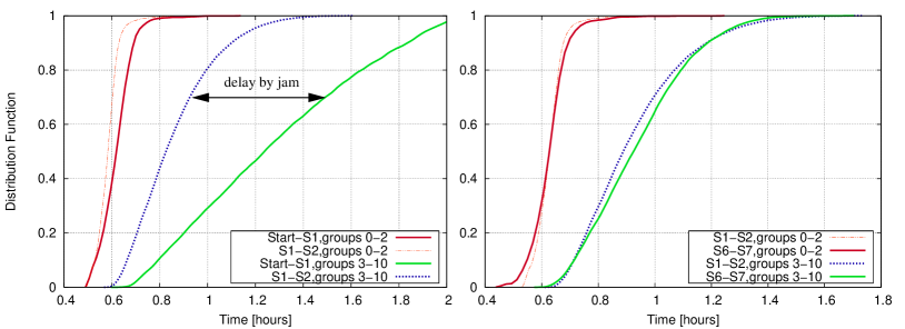
Figure 4: Distribution functions of the split times from the start to Station S1 (left), S1 to S2 (left and right), and S6 to S7 (right), shown separately for the fastest groups (elite and groups 1 and 2) and the remaining groups 3 to 10. All three sections take about the same time. Major jams occur only for the groups 3 to 10 and only between the start and S1.

As in the real event, we simulated a mass start. While the initial starting configuration dissolves relatively quickly, massive jams form at the beginning of the gradient section, particularly at the route divide (inset of Fig. 3). In summary, the delays due to the jams accumulated up to 40 minutes for the last starting groups which agrees with the macroscopic flow-based analysis of the split-time data (Fig. 4).

4 Conclusion

Using the open-software MovSim, we have quatitatively reproduced the congestions and stop-and-go waves on the first ten kilometers of the Vasaloppet Race 2012. The jams leading to a delay of up to 40 minutes are caused a steep uphill section and a simultaneous reduction of the number of tracks. Further simulations have also shown that eliminating the worst bottlenecks by locally adding a few tracks only transfers the jams to locations further downstream. In contrast, replacing the mass start (which is highly controversial) by a wave start with a five-minute delay between the starting groups would essentially eliminate the jams without the need to reduce the total number of participants.

References

- (1) P. Ahmadi, Analysis of traffic patterns for large scale outdoor events a case study of vasaloppet ski event in sweden, Thesis, Royal Institute of Technology.
- (2) M. Treiber, Crowd Flow Modeling of Athletes in Mass Sports Events - a Macroscopic Approach. In this proceedings.
- (3) M. Treiber, A. Kesting, Traffic Flow Dynamics: Data, Models and Simulation, Springer, Berlin, 2013.
- (4) A. Kesting, R. Germ, M. Budden, M. Treiber, MovSim – Multi-model Open-source Vehicular Simulator, www.movsim.org.