Crowd Flow Modeling of Athletes in Mass Sports Events - a Macroscopic Approach

Abstract

. We propose a macroscopic model in form of a dispersion-transport equation for non-congested flow of the athletes which is coupled to a kinematic-wave model for congested flow. The model takes into account the performance (i.e., free-flow speed distributions) of the athletes in the different starting groups. The model is calibrated and validated on data of the German Rennsteig Half Marathon 2012 and the Swedish Vasaloppet 2012 cross-country ski race. Simulations of the model allow the event managers to improve the organization by determining the optimum number of starting groups, the maximum size of each group, whether a wave start with a certain starting delay between the groups is necessary, or what will be the effects of changing the course. We apply the model to simulate a planned course change for the Rennsteig Half Marathon 2013, and determine whether critical congestions are likely to occur.

1 Introduction

Mass-sport events for runners, cross-country skiers, or other athletes, are increasingly popular. Prominent examples include the New York Marathon, the Vasaloppet cross-country ski race in Sweden, and the nightly inline-skating events taking place in nearly every major European city. Due to their popularity (the number of participants is typically in the thousands, sometimes in the ten thousands), “traffic jams” occur regularly (Fig. 1). They are not only a hassle for the athletes (since the time is ticking) but also pose organisational or even safety threats, e.g., because a spillback from a jam threatens to overload a critical bridge. Nevertheless, scientific investigations of the athletes’ crowd flow dynamics TreiberKesting-Book are virtually nonexisting.

Figure 1: Jams at the Swedish Vasaloppet cross-country race 2012 (left) and at the Rennsteig Marathon 2012 (right).

The crowd dynamics can be described by two-dimensional active-particle systems Helbing-01aa . Unlike the situation in general pedestrian traffic, the flow is unidirectional since all athletes share the same destination (the finishing line). This means, the dynamics is equivalent to that of mixed unidirectional vehicular traffic flow which may be lane-based, as in cross-country ski races in the classic style TGF13-ski , or not, as in running events but also in mixed vehicular traffic flow in many developing countries Arasan-mixedTraffic . The uni-directionality allows to simplify the mathematical description to a macroscopic, one-dimensional model for the motion along the longitudinal (arc-length) coordinate.

In this contribution, we formulate a macroscopic dispersion-transport model for free flow which is coupled to a kinematic-wave model for congested flow. We calibrate and validate the model by data of the Rennsteig 2012 Half Marathon and the Vasaloppet 2012 and apply it to simulate the effects of a planned course change for the next Rennsteig Half Marathon 2013 to avoid the overloading of a critical bridge.

In the next section, we develop the macroscopic model and show its workings on data of past running and ski events. In Section 3, we apply it to simulate organisational changes for the Rennsteig Half Marathon 2013. Finally, Sec. 4 gives a discussion.

2 The Macroscopic Model

Our proposed macroscopic model has two components for free and congested traffic, respectively. Since, in free traffic, individual performance differences translate into different speeds, we formulate the free-traffic part as a multi-class model. In contrast, “everybody is treated equal” in congested traffic, so a simple single-class kinematic-wave model is sufficient. During the simulation, the free-traffic part provides the spatio-temporally changing traffic demand (athletes per second). A congestion arises as soon as the local demand exceeds the local capacity. The resulting moving upstream boundary of the jam is subsequently described by standard shock-wave kinematics.

2.1 Free Traffic Flow

In most bigger mass sports events, the athletes are classified according to performance into starting groups. All groups start either simultaneously (“mass start”, Fig. 2 (a)), or sequentially with fixed delays between the groups which, then, are also called waves (“wave start”, Fig. 2 (b)).

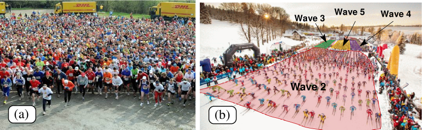
Figure 2: Two possible starting schemes. (a) mass start (Rennsteig Marathon 2012); (b) wave start (Jizerska Padesatka 50 km, 2012).

Generally, each athlete wears an individual RFID chip recording the starting and finishing time, and also split times when passing refreshment stations along the course. The information of the starting groups is highly useful since the speed distribution within each group is much narrower than that for the complete field. Thus, by considering each group individually, the model makes more precise predictions.

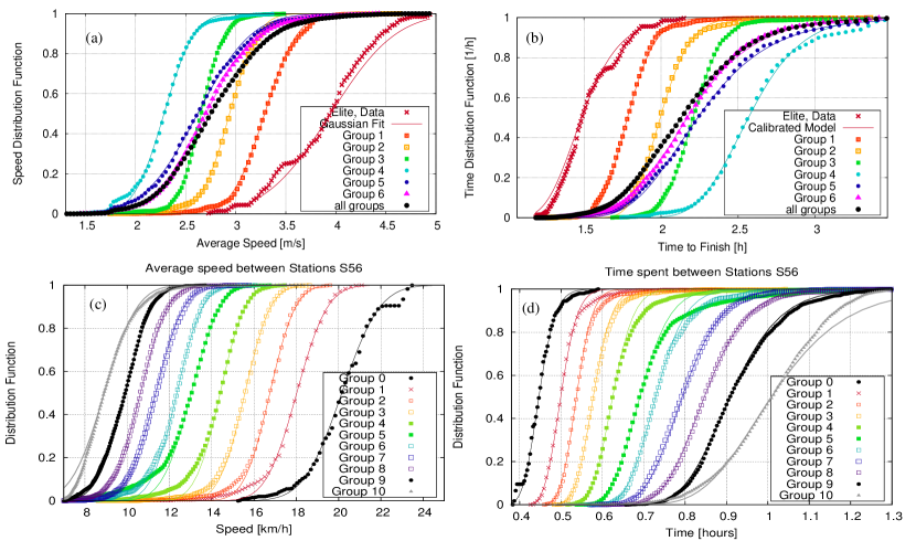
Figure 3: Distribution of the average speeds (left) and times (right) of the different starting groups at the Rennsteig Half Marathon 2012 (whole race, top) and at the Vasaloppet 2012 (a 9 km section between the stations 5 and 6, bottom). Symbols: data; curves: model.

Figure 3 shows the distributions of the final times of the German Rennsteig Half Marathon and the time for a section of the Vasaloppet 2012 where no major jams are observed. We fitted the data of each group by Gaussians parameterized, for reasons of robustness, by the median and the inter-quartile gap instead of the arithemic mean and standard deviation. We infer that, in the absence of major disturbances, the speed distribution within each group is nearly Gaussian. Significant deviations are only observed (i) for the small elite groups due to platooning, (ii) for the low-speed tails. (Generally, the low-speed tails are fatter compared to Gaussians. However, at the Vasaloppet, the slowest athletes are taken out of the race thus reversing this effect.)

Using the normal kinematic relation $T=L/v$ for the time $T$ that athletes of group $k$ take to cover the distance $L$ at speed $v$, we obtain by elementary probability theory following relation between the density functions $f^{v}_{k}(v)$ of the speed and the (non-Gaussian) density function $f^{T}_{k}(T|L)$ of the needed time,

$$f^{T}_{k}(T|L)=\frac{L}{T^{2}}f^{v}_{k}\left(\frac{L}{T}\right).$$ (1)

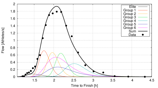
Figure 4: Partial flows $Q_{k}(x,t)$ of the different starting groups (mass start) at the finish at 21.1 km (colored curves) and total flow according to (2) (thick curve) compared with the actual flow (data points).

Finally, we assume that the relative performance of an athlete persists throughout the race. In other words, in free traffic, a fast runner remains fast and a slow athlete slow. This means, the flow dynamics obeys a dipersion rather than a diffusion equation. Specifically, we assume constant speed distributions on flat terrain and identical relative speed changes for inhomogeneities such as uphill or downhill gradients. In the following, we will assume a flat terrain, for notational simplicity.

Denoting the number of athletes in each group by $n_{k}$ and assuming a wave start where group $k$ starts a time delay $\tau_{k}$ after the starting gun goes off (indicating the start of the first and elite waves), the free-traffic demands $Q_{\rm free}(x,t)$ and densities $\rho_{\rm free}(x,t)$ read

$$Q_{\rm free}(x,t) = \sum_{k}Q_{k}(x,t-\tau_{k}),\quad Q_{k}(x,t)=n_{k}f^{T}_{k}(t|x),$$ (2)

$$\rho_{\rm free}(x,t) = \sum_{k}\rho_{k}(x,t-\tau_{k}),\quad\rho_{k}(x,t)=\frac{t}{x}\,Q_{k}(x,t),$$ (3)

where $Q_{k}$ and $\rho_{k}$ are set to zero for time arguments $t-\tau_{k}\leq 0$. Figure 4 shows that the model prediction for the total traffic demand $Q_{\rm free}(x,t)$ at the finish line fits well with the data (possibly, the small deviation at the peak is due to congestions). Thus, we are now able to estimate the free-flow traffic demand upstream of a congestion at any location and at any time during the race. Moreover, we now can anticipate the consequences of organisational changes such as realizing a wave start rather than a mass start (Fig. 5).

Figure 5: Simulated effect of a wave start on the local flow of athletes (all starting groups) at different locations from $x=2\,500\,\mathrm{m}$ to the finish. (a) Reference (mass start), (b) delay of 5 min.

2.2 Kinematic-Wave Model for Congested Crowds

We propose a quasi-onedimensional Lighthill-Whitham-Richards model with a triangular fundamental diagram. In terms of the local capacity $C(x)$ (maximum number of athletes per second that can pass a cross section at location $x$), the free-flow speed $V_{0}$, and the maximum local one-dimensional density (athletes per meter) $\rho_{\rm max}(x)$, the fundamental diagram can be expressed by TreiberKesting-Book

$$Q_{e}(\rho)=\max\left[V_{0}\rho,\frac{C(\rho_{\rm max}-\rho)}{\rho_{\rm max}-C/V_{0}}\right].$$ (4)

Notice that the observed capacity $C$ increases weakly with the maximum speed $V_{0}$ such that $V_{0}$ essentially cancels out in the congested branch of (4). A traffic breakdown arises if, at any location or time, the free-flow demand $Q_{\rm free}(x,t)$ exceeds the local capacity $C_{B}$ at a bottleneck $x=x_{B}$ (where the capacity is at a local minimum). The resulting congested traffic region has a one-dimensional density

$$\rho_{\rm cong}(x)=\rho_{\rm max}(x)\left(1-\frac{C_{B}}{C(x)}\right)+\frac{C_{B}}{V_{0}}.$$ (5)

The congestion has a stationary downstream front at the bottleneck location $x_{B}$ while the upstream front $x_{\rm up}(t)$ is moving according to the shock-wave formula

$$\frac{{\rm d}x_{\rm up}}{{\rm d}t}=\frac{C_{B}-Q_{\rm free}(x,t)}{\rho_{\rm cong}(x)-\rho_{\rm free}(x,t)}.$$ (6)

The congestion dissolves as soon as $x_{\rm up}(t)$ crosses $x_{B}$ in the downstream direction. Finally, the free-traffic flow downstream of the congested region has a constant flow $Q_{\rm free}^{\rm down}(x,t)=C_{B}$ equal to the bottleneck capacity.

Both the local capacities and maximum densities are proportional to the local width $w(x)$ of the course:

$$C(x)=J_{\rm max}w(x),\quad\rho_{\rm max}(x)=\rho_{\rm max}^{\rm 2d}w(x).$$ (7)

The maximum flow density (specific capacity) $J_{\rm max}$ and the maximum 2d density $\rho_{\rm max}^{\rm 2d}$ are model parameters depending on the kind of race and on the local conditions (e.g., gradients). From past congestions, we can estimate $\rho_{\rm max}^{\rm 2d}=2\,\mathrm{m^{-2}}$ and $J_{\rm max}=1.5\,\mathrm{(ms)^{-1}}$ for running competions on level terrain (which is comparable to normal unidirectional pedestrian flows), and $\rho_{\rm max}^{\rm 2d}=0.7\,\mathrm{m^{-2}}$, $J_{\rm max}=0.6\,\mathrm{(ms)^{-1}}$ for level-terrain cross-country ski events.

3 Simulating Scenarios for a Marathon Event

At the 2012 Rennsteig Half Marathon, there were six starting groups. The last group contained significantly more participants. For 2013, the managers plan eight groups of equal size $n_{k}\leq 850$, with the first five groups sorted to performance, and the last three groups available for the runners for which no previous performance are known or who registered too late. Based on the 2012 data, we set the average speeds to $v_{1}=3.5\,\mathrm{m/s}$, $v_{2}=3.1\,\mathrm{m/s}$, $v_{3}=2.7\,\mathrm{m/s}$, $v_{4}=2.4\,\mathrm{m/s}$, $v_{5}=2.1\,\mathrm{m/s}$, and $v_{6}=v_{7}=v_{8}=2.7\,\mathrm{m/s}$. All speed variances are assumed to be $\sigma_{v}^{2}=0.15\,\mathrm{m^{2}/s^{2}}$.

Due to external constraints, the course of the 2013 Marathon must be changed. There are several options:

• Scenario 1: Mass start. The 5 m wide starting section has a capacity of 7 athletes/s. The first bottleneck at $x=1\,000\,\mathrm{m}$ is a 7% uphill gradient section of 4.5 m width. At $x=2\,200\,\mathrm{m}$, the athletes encounter a 3.5 m wide downhill section. The critical bottlenecks, however, consist of a bridge at $x=3\,000\,\mathrm{m}$ (level, 3 m wide), and, 100 m afterwards, a steep uphill gradient (11%) where the course has a width of 3.5 m.

• Scenario 1a: As Scenario 1, but wave start with a delay of 300 s per wave

• Scenario 1b: As Scenario 1a, but the capacity of the starting section has been reduced to 5.5 athletes/s.

• Scenario 2: The course is reorganized such that the 7% gradient is at $x=1\,400\,\mathrm{m}$, the downhill bottleneck at $x=2\,700\,\mathrm{m}$, and the bridge with the subsequent steep uphill section at $x=5\,700\,\mathrm{m}$ and 5 800 m, respectively.

Based on past experience, the maximum 2d density is set to $\rho_{\rm max}^{\rm 2d}=2\,\mathrm{m^{-2}}$ and the specific capacities to $J_{\rm max}=1.5\,\mathrm{(ms)^{-1}}$ for level sections (including the bridge), and $1.2\,\mathrm{(ms)^{-1}}$, $1.0\,\mathrm{(ms)^{-1}}$, and $1.3\,\mathrm{(ms)^{-1}}$ for the 7%, 11%, and the downhill gradients, respectively. Figure 6 displays the resulting fundamental diagrams for the bridge (capacity $C=4.5\,\mathrm{s^{-1}}$) and the subsequent uphill section ($C=3.5\,\mathrm{s^{-1}}$)

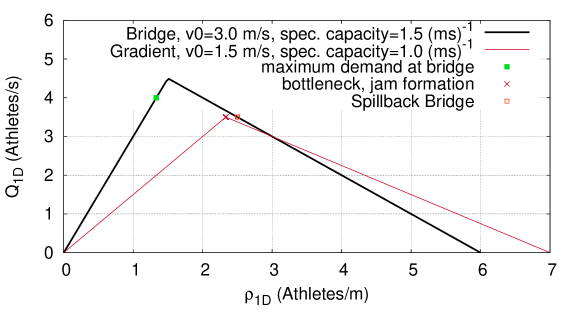
Figure 6: Fundamental diagram for different situations of the simulation of the Rennsteig Half Marathon 2013 (see the main text for details.)

While some congestions are unavoidable, we must require that there is no significant congestion on the 60 m long bridge itself because this may result in dangerous overloading.

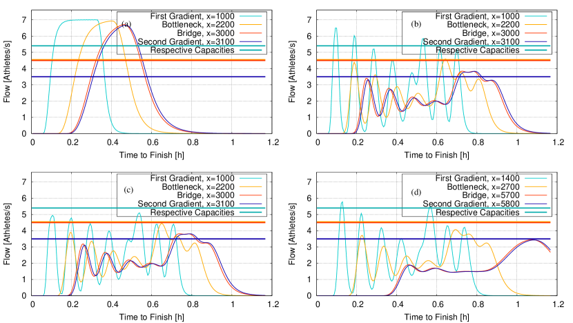
Figure 7: Two simulated scenarios for the Rennsteiglauf Half Marathon 2013. The horizontal lines give the capacities of the various bottlenecks of the course, and the curves of the same color the predicted demands at these positions.

Figure 7 shows the main results: With a mass start (Fig. 7(a)), massive jams will form at and upstream of all the bottlenecks, including a spillback to the bridge, so this is no option. Adopting a wave start (Fig. 7(b)) reduces the congestion at the first bottleneck to a tolerable level. Furthermore, jams are no longer expected at the downhill bottleneck while the bridge itself has even capacity to spare. However, the demand exceeds the capacity of the steep uphill section leading to a supply-demand mismatch of up to about 150 athletes (the area between the blue curve and the blue capacity line of Fig. 7(b)). This corresponds to a jam of about 150 m, i.e., there is a spillback with a density of 2.5 athletes/m (cf. Fig. 6) onto the bridge. Reducing the initial capacity of the starting field to 5.5 athletes/s (Fig. 7(c)) does not help much in this situation. Only a rearrangement of the course with the bridge section located further away from the start yields a significant improvement with the only (minor) jam expected at the uncritical first bottleneck.

4 Discussion

We have proposed a macroscopic dispersion-transport model that allows managers of mass-sports events to assess the implications of changing the course, or the spatio-temporal organization of the start, without prior experiments. As a general rule, critical bottlenecks should be moved as far away from the start as possible. If the situation remains critical, a wave start and/or a restriction of the number of participants will be necessary.

References

- (1) M. Treiber, A. Kesting, Traffic Flow Dynamics: Data, Models and Simulation, Springer, Berlin, 2013.
- (2) D. Helbing, Traffic and related self-driven many-particle systems, Reviews of Modern Physics (2001) 1067–1141.
- (3) M. Treiber, R. Germ, A. Kesting, From Drivers to Athletes – Modeling and Simulating Cross-Country Skiing Marathons. In this proceedings.
- (4) V. Arasan, R. Koshy, Methodology for modeling highly heterogeneous traffic flow, Journal of Transportation Engineering 131 (7) (2005) 544–551.