Reflection From the Strong Gravity Regime in a $z=0.658$ Gravitationally Lensed-Quasar

Abstract

The co-evolution of a supermassive black hole with its host galaxy[1] through cosmic time is encoded in its spin[2, 3, 4]. At $z>2$, supermassive black holes are thought to grow mostly by merger-driven accretion leading to high spin. However, it is unknown whether below $z\sim 1$ these black holes continue to grow via coherent accretion or in a chaotic manner[5], though clear differences are predicted[3, 4] in their spin evolution. An established method[6] to measure the spin of black holes is via the study of relativistic reflection features[7] from the inner accretion disk. Owing to their greater distances, there has hitherto been no significant detection of relativistic reflection features in a moderate-redshift quasar. Here, we use archival data together with a new, deep observation of a gravitationally-lensed quasar at $z=0.658$ to rigorously detect and study reflection in this moderate-redshift quasar. The level of relativistic distortion present in this reflection spectrum enables us to constrain the emission to originate within $\lesssim 3$ gravitational radii from the black hole, implying a spin parameter $a=0.87^{+0.08}_{-0.15}$ at the $3\sigma$ level of confidence and $a>0.66$ at the $5\sigma$ level. The high spin found here is indicative of growth via coherent accretion for this black hole, and suggests that black hole growth between $0.5\lesssim z\lesssim 1$ occurs principally by coherent rather than chaotic accretion episodes.

When optically-thick material, e.g. an accretion disc, is irradiated by hard X-rays, some of the flux is reprocessed into an additional ‘reflected’ emission component, which contains both continuum emission and atomic features. The most prominent signature of reflection from the inner accretion disc is typically the relativistic iron K$\alpha$ line (6.4–6.97$\rm\thinspace keV$; rest frame)[8] and the Compton reflection hump[7] often peaking at $20-30$$\rm\thinspace keV$ (rest-frame). However, the deep gravitational potential and strong Doppler shifts associated with regions around black holes will also cause the forest of soft X-ray emission lines in the $\sim 0.7-2.0$$\rm\thinspace keV$ range to be blended into a smooth emission feature, providing a natural explanation for the “soft-excess” observed in the X-ray spectra of nearby active galactic nuclei (AGNs)[9, 10]. Indeed, both the iron line and the soft excess can be used to provide insight into the nature of the central black hole and to measure its spin[10]. Prior studies have revealed the presence of a soft-excess in $\gtrsim 90\%$ of quasars at[11, 12] $z\lesssim 1.7$, and broad Fe-lines are also seen in $\lesssim 25\%$ of these objects[11, 13], suggesting that reflection is also prevalent in these distant AGNs. However, due to the inadequate S/N resulting from their greater distances, the X-ray spectra of these quasars were necessarily modeled using simple phenomenological parameterizations[12, 14].

Gravitational lensing offers a rare opportunity to study the innermost relativistic region in distant quasars[15, 16], by acting as a natural telescope and magnifying the light from these sources. Quasars located between $0.5\lesssim z\lesssim 1$ are considerably more powerful than local Seyferts and are known to be a major contributor to the Cosmic X-ray background[17], making them objects of particular cosmological importance. 1RXS J113151.6-123158 (hereafter RX J1131-1231) is a quadruply imaged quasar at redshift $z=0.658$ hosting a supermassive black hole ($\rm M_{BH}\sim 2\times 10^{8}\hbox{$\rm\thinspace M_{\odot}$}$)[18] gravitationally lensed by an elliptical galaxy at $z=0.295$ [19]. X-ray and optical observations exhibited an intriguing flux-ratio variability between the lensed images, which was subsequently revealed to be due to significant gravitational micro-lensing by stars in the lensing galaxy[15, 16].

Taking advantage of gravitational micro-lensing techniques, augmented by substantial monitoring with the Chandra X-ray observatory, a tight limit of the order of $\sim 10$ gravitational radii (${\rm r_{g}=GM/c^{2}}$) was placed[20] on the maximum size of the X-ray emitting region in RX J1131-1231, indicative of a highly compact[21] source of emission ($\lesssim 3~{}{\rm billion~{}km}$, or $\lesssim 20~{}{\rm AU}$). The lensed nature of this quasar provides an excellent opportunity to study the innermost regions around a black hole at a cosmological distance (the look-back time for RX J1131-1231 is $\sim 6.1$ billion years), and to this effect Chandra and XMM-Newton have to-date accumulated nearly 500$\rm\thinspace ks$ of data on RX J1131-1231.

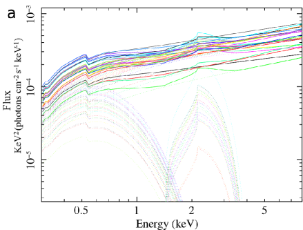
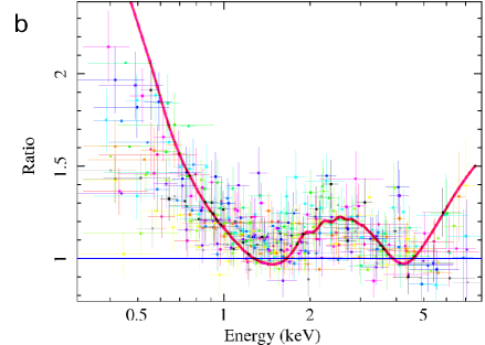
Figure 1: a: Phenomenological models for all 27 Chandra observations of Image B fit with a DISKBB component to mimic the soft excess as well as a RelLine line profile to account for the residuals in the 2-4$\rm\thinspace keV$ range and a power-law for the continuum. The normalisation of the various components as well as as the power-law indices are allowed to vary between epochs, however, the intrinsic column density, the ionisation state (related to the centroid of the line), emissivity profile and inclination of the disk are assumed to be unchanging between the various epochs. b: Ratio plot made in a similar manner as in Extended Data Fig. 2 for all 27 epochs. The solid magenta line is the baseline theoretical best fit model-to-power-law ratio expected from the self-consistent REFLIONX model found for epoch 23. The data have been rebinned for visual clarity.

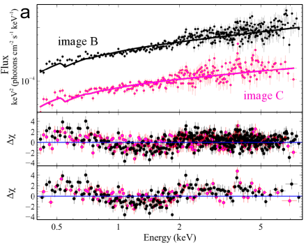
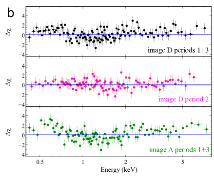
Figure 2: a: Co-added Chandra spectra of Images B (black) and C (magenta) during all observations. The spectra are shown fit with a simple power-law, and the residuals to this model are shown in units of 1$\sigma$ deviations in the middle panel. The data in the bottom panel have been rebinned for display purposes. (b:) Co-added spectra of Periods 1 and 3 (black) and Period 2 (magenta) of Image-D shown as residuals to a simple power-law together with Gaussians similar to that shown in ref[16]. The residuals to this model are shown in units of 1$\sigma$ deviations. The bottom panel shows similar residuals for the corresponding Periods 1+3 of Image-A. The data have been rebinned for display purposes.

Starting with the Chandra data, fits with a model consisting of a simple absorbed powerlaw continuum, both to the data from individual lensed images (Extended Data Fig. 1) and to the co-added data (Extended Data Fig. 2,4,5), reveal broad residual emission features both at low energies ($\lesssim 2$ keV rest frame, the “soft-excess”) and around the iron K energies (3.5–7 keV rest frame), characteristic signatures of relativistic disk reflection[10, 23]. To treat these residuals, we consider two template models based on those commonly used to fit the spectra of Seyferts[24, 6] and stellar mass black hole binaries[25], and which have also at times been used to model local quasars[26]. The first is a simple phenomenological combination of a power-law, a soft-thermal disk and a relativistic Fe-line component (baseline-simple), and the second employs a self-consistent blurred-reflection model together with a power-law (baseline-reflection). In addition, both models include two neutral absorbers; the first to account for possible intrinsic absorption at the redshift of the quasar; and the second to account for Galactic absorption.

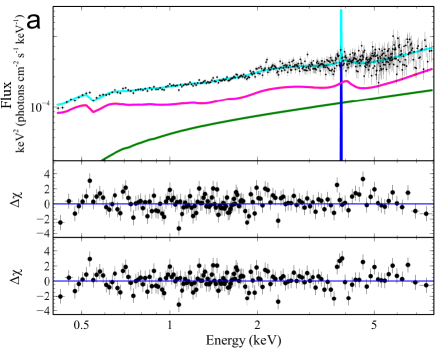
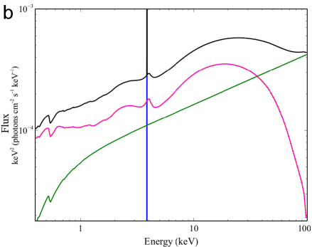
Figure 5: a: Co-added spectrum of all Chandra epochs. The spectrum was fit with a physically motivated, self consistent model for both the soft-excess and the broad iron line. The residuals to the model is shown in the middle panel. The REFLIONX, power-law and narrow Gaussian components are shown in magenta green and blue respectively, with the total model shown in cyan. The bottom panel shows the residuals without the narrow Gaussian component. (Panel b:) Extrapolated model showing a reflection dominated continuum. The data was rebinned for display purposes.

We first statistically confirm the presence of reflection features in RX J1131-1231 using baseline-simple. Least-squares fits were made to all the individual Chandra spectra of image-B simultaneously, allowing only the normalisations of the various components and the power-law indices to vary (Extended Data Fig. 1). The thermal-component, used here as a proxy for the soft-excess, is required at $>10\sigma$ and an F-test indicates that the addition of a relativistic emission line to the combined Chandra data of image-B is significant at greater than the 99.9% confidence level. Tighter constraints ($>5\sigma$) on the significance of the relativistic iron line can be obtained by co-adding all Chandra data to form a single, time-averaged spectrum representative of the average behaviour of the system (Figure 2 and Extended Data Fig. 5).

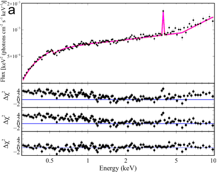
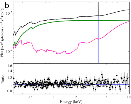
Figure 6: a: XMM-Newton EPIC-PN spectrum of RX J1131-1231. (Top) unfolded spectrum showing the total broken powerlaw together with a soft excess and narrow Gaussian in magenta. The second panel from the top shows the residuals upon removal of the soft component, the narrow line and break in the powerlaw. The following panel shows the fit with the addition of a break in the powerlaw and the bottom panel shows the best phenomenological fit to the XMM-Newton data. b: XMM-Newton data now fit with the Baseline-reflection model. The reflection component is again shown in magenta, with the total, powerlaw and narrow line shown in black, green and blue respectively. The bottom panel shows the ratio to this model. The data have been rebinned for display purposes.

The XMM-Newton observation also shows the clear presence of a soft excess below $\sim 1.2$$\rm\thinspace keV$, again significant at $>5\sigma$, and thanks to its high effective area above $\sim 5\hbox{$\rm\thinspace keV$}$, it also displays the presence of a hardening at high energies (Extended Data Fig. 6). An F-test indicates that a break in the powerlaw at $\sim 5$$\rm\thinspace keV$ (Figure 2) is significant at the $3.6\sigma$ level of confidence. This hardening is consistent with the expectation of a reflection spectrum and can be characterised with the Compton reflection hump[7].

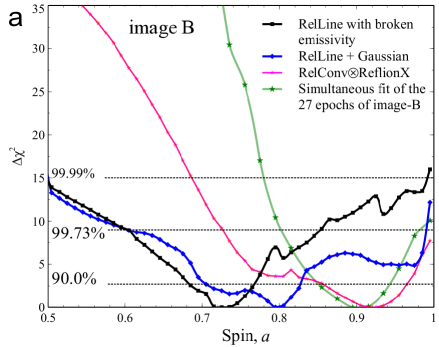
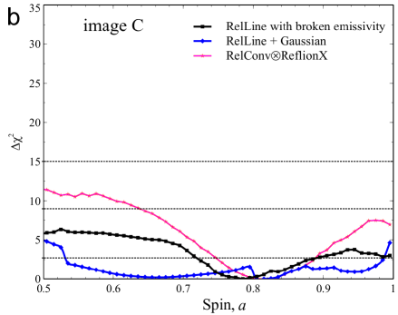
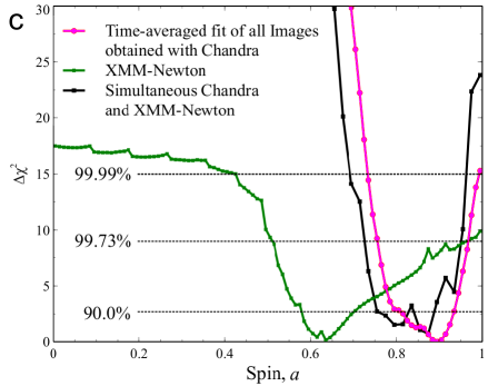
Figure 3: Goodness-of-fit versus spin parameter for the co-added spectrum of Images-B (panel a) and C (panel b). By co-adding the spectra we are probing the time averaged behaviour of the reflection spectrum. Fits were made with the spin parameter varying from 0.495 to 0.995 in steps of 0.01. The blue contours were made using the relativistic line model RelLine assuming a broken emissivity profile and a further narrow Gaussian line at 6.4$\rm\thinspace keV$. The black contours assumes a broken emissivity without an extra narrow Gaussian line. Finally, the magenta contours are for the self-consistent REFLIONX model together with the RelConv blurring kernel and a Gaussian line at 6.4$\rm\thinspace keV$ (see text for details). We have also included for Image-B, the contour (green) found for the time-resolved analyses described in §6. Panel c: Co-added spectrum of all Chandra (magenta contours), XMM-Newton (green contours) and simultaneous data (black contour). These contours are made with the Baseline-reflection model. The dotted lines show the 99.99%, 99.73% ($3\sigma$) and 90% confidence limit.

The unprecedented data quality for this moderate-$z$ quasar ($\sim$100,000 counts in the 0.3-8 $\rm\thinspace keV$ energy range from each of the Chandra and XMM-Newton datasets) enables us to apply physically motivated, self-consistent models for the reflection features. We proceed by using the baseline-reflection model to estimate the spin parameter through a variety of analyses, including time-resolved and time-averaged analyses of individual Chandra images, utilising its superior angular resolution, and through analysis of the average spectrum obtained from all four lensed images with XMM-Newton. During the time-resolved analysis, the black hole spin parameter as well as the disk inclination and emissivity profile were kept constant from epoch to epoch, while the normalisations of the reflection and power-law components, as well as the ionisation state of the disk and the power-law indices were allowed to vary between epochs (see online SI for further details). In all cases, we obtain consistent estimates for the black hole spin, which imply RX J1131-1231 hosts a rapidly rotating black hole (Extended Data Fig. 3 and Extended Data Tables 1,2). Finally, in order to optimise the S/N and obtain the best estimate of the spin parameter we fit the combined Chandra and XMM-Newton data of RX J1131-1231 simultaneously with the baseline-reflection model and find $a=0.87^{+0.08}_{-0.15}~{}{\rm Jc/GM^{2}}$ at the $3\sigma$ level of confidence ($a>0.66~{}{\rm Jc/GM^{2}}$ at the $5\sigma$ level; Figure 3).

The tight constraint on the spin of the black hole in this gravitationally lensed quasar represents a robust measurement of black hole spin beyond our local universe. The compact nature of the X-ray corona returned by the relativistic reflection model used herein confirms the prior micro-lensing analysis[15, 16], and hence moves the basic picture of X-ray emission in quasars away from large X-ray coronae[27] that may blanket at least the inner disk, and more towards a compact emitting region in the very innermost parts of the accretion flow, consistent with models for the base of a jet[28].

In addition to constraining the immediate environment and spin of the black hole, the analysis presented herein has implications for the nature of the Cosmic X-ray background. The best-fit baseline-reflection model to the time-averaged Chandra and XMM-Newton spectra (Extended Data Figs. 5,6) suggest that the source is at times reflection dominated, i.e., we find the ratio of the reflected to the illuminating continuum in the Chandra (XMM-Newton) data to be ${\rm f_{reflect}/f_{illum}}=2.3\pm 1.2~{}(0.47\pm 0.15)$ in the 0.1 – 10$\rm\thinspace keV$ band (local frame; Extended Data Table 2). However, it must be noted that uncertainties in the size of the microlensed regions could affect the absolute value of this ratio. Nonetheless, this analysis clearly demonstrates the presence of a significant contribution from a reflection component to the X-ray spectrum of this $z=0.658$ quasar. The properties of RX J1131-1231 are consistent[11, 13, 12, 14, 16] with the known observational characteristics of quasars at $0.5\lesssim z\lesssim 1$, and our results suggest that the relativistic reflection component from the large population of unobscured quasars expected in this epoch[17] could significantly contribute in the 20–30$\rm\thinspace keV$ band of the Cosmic X-ray background.

Although questions have previously been raised over whether reflection is a unique interpretation for the features observed in AGNs, the amassed evidence points towards this theoretical framework[24, 29], and reached culmination with the launch of NuSTAR and the strong confirmation of relativistic disk reflection from a rapidly spinning supermassive black hole at the centre of the nearby galaxy NGC 1365[6]. Nonetheless, there still remain possible systematic uncertainties, for example, due to the intrinsic assumption that the disk truncates at the innermost stable circular orbit. Simulations have been performed specifically aimed at addressing the robustness of this assumption[30], which find that emission within this radius is negligible, especially for rapidly rotating black holes, as is the case here.

The ability to measure cosmological black hole spin brings with it the potential to directly study the co-evolution of the black hole and its host galaxy[1]. The ultimate goal is to measure the spin in a sample of quasars as a function of redshift and to make use of the spin distribution as a window on the history of the co-evolution of black hole and galaxies[4]. Our measurement of the spin in RX J1131-1231 is a step along that path, and introduces a possible means to begin assembling a sample of supermassive black hole spins at moderate red-shift with current X-ray observatories.

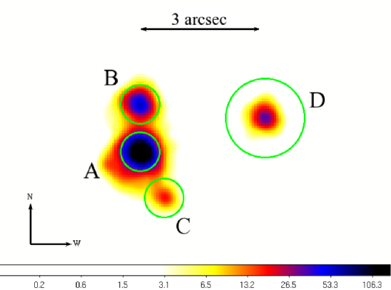
Figure 1: Chandra image of RX J1131-1231. This representative image of a single epoch was made using subpixel techniques in the 0.3-8$\rm\thinspace keV$ energy range (SI) and is shown here smoothed with a Gaussian ($\sigma=$ 0.25”). The green circles show the source extraction regions. For images A–C, we used a radius of 0.492”, whereas the source region for image D was set to 0.984”. Individual source and background regions were made for all 30 observations and spectra were extracted from the unsmoothed images.

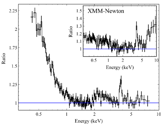
Figure 2: Broad iron line, soft and hard excess in RX J1131-1231. The main panel shows the co-added Chandra data over all epochs for all 4 images. The data was fit in a phenomenological manner with a model consisting of an absorbed power-law with an index of $\Gamma=1.60\pm 0.04$ for the continuum, a thermal disk component with a temperature of $0.19\pm 0.02$$\rm\thinspace keV$ to account for the soft-excess, and a broad relativistic line with energy constrained to lie between 6.4–6.97$\rm\thinspace keV$ (rest-frame; the Baseline-simple model). The ratio is shown after setting the normalisation of the disk, relativistic line and narrow line component to zero in order to better highlights these features. The inset shows the XMM-Newton data fit with a $\Gamma=1.83$ powerlaw. The best fit, phenomenological model for the XMM-Newton data requires the presence of a soft excess which can again be characterised by a thermal disk component with a temperature of $0.22\pm 0.03\hbox{$\rm\thinspace keV$}$, a powerlaw with an index $\Gamma=1.83^{+0.07}_{-0.03}$ up to a break at $E_{\rm break}=5.5^{+0.5}_{-2.2}\hbox{$\rm\thinspace keV$}$, at which point it hardens to $\Gamma=1.28^{+0.33}_{-0.19}$. This hardening is interpreted as the Compton reflection hump. Both co-added spectra shown here probe the time-averaged behaviour of RX J1131-1231. Quoted errors refers to the 90% confidence limit and the error bars are 1$\sigma$.

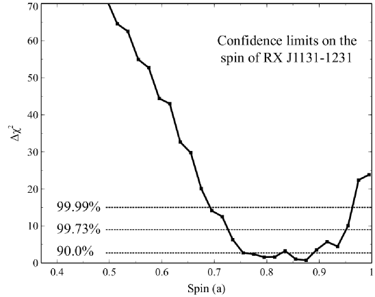
Figure 3: Goodness-of-fit versus the spin parameter of the supermassive black hole in RX J1131-1231. Fits were made with the spin parameter varying from 0.495 to 0.995 in steps of 0.02 with all all parameters of the model allowed to vary. The contour was made adopting a model consisting of a power-law together with a relativistic blurred reflection by an accretion disk, as well as two neutral absorbers; one at the redshift of the quasar and another local to our Galaxy (the Baseline-reflection model). The fit was made to the co-added spectra from both XMM-Newton and Chandra simultaneously, with the assumption that the spin of the black hole, the inclination of the accretion disk and the total hydrogen in our line of sight does not change between observations. The dotted lines show the 99.99%, 99.73% ($3\sigma$) and 90% confidence limit where it becomes clear that the supermassive black hole in RX J1131-1231 must be rotating with a spin $a=0.87^{+0.08}_{-0.15}~{}{\rm Jc/GM^{2}}$ at the $3\sigma$ level of confidence.

Methods Summary

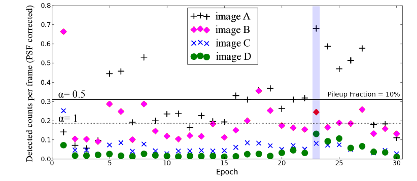
Figure 7: Detected Counts per Frame as a function of observation epoch. The counts have been PSF-corrected in order to account for the size of the extraction region. As such, the counts presented are approximately a factor of 1.69, 1.71, 1.69 and 1.21 higher that that observed for images A, B, C and D respectively. We show with solid and dotted horizontal lines the expected 10% pileup fraction assuming a grade migration parameter of $\alpha=1$ and 0.5, respectively. The highlighted epoch corresponds to that used in the in-depth study of possible spectral distortions due to pile-up/cross contamination. We use this epoch to assess the implication of high count rate on our results as it presents the greatest chance of cross-contamination due to the peak brightness of Image-A. The work highlighted in the Online methods clearly shows that the features observed in this epoch is consistent with those observed in all, fainter, observations.

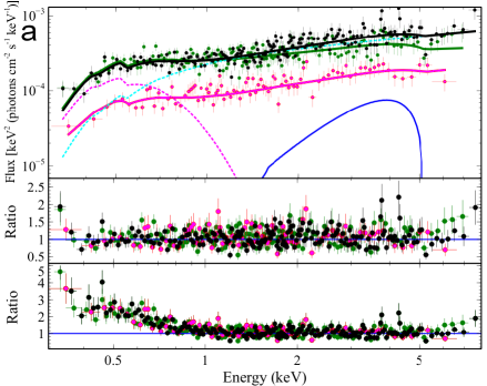
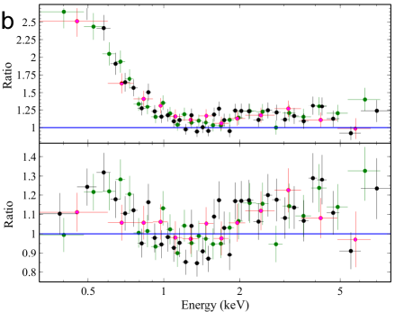
Figure 8: a: Chandra Spectra of images-B, C and D from the observation made on 2009 November 28. This observation is highlighted in Extended Data Fig. 1 and is representative of the brightest Chandra epochs used in this work. It is also the observation in which Image-A is at its brightest and therefore presents the largest chance of cross contamination as sources are only $\sim 1$$\rm\thinspace arcsec$ apart. The spectra were fit phenomenologically with a combination of a power-law, DISKBB and RelLine line profile to describe the continuum, soft excess and iron emission feature respectively. The ratio to the model are shown both with (centre) and without (bottom) the disk component representing the soft-excess. The spectra of image-B, C and D are shown in black, magenta and green respectively. The power-law, DISKBB and RelLine components for image-B are shown in cyan, magenta, and blue respectively with the total model shown as solid lines for the 3 images. b: Data-to-model ratio obtained after removing the RelLine and DISKBB components (top) and after refitting with a single power-law (bottom). The ratio for images B, C and D are shown in black, magenta and green respectively and have been rebinned for display purposes. Despite the different flux levels between these 3 images, it is clear that the residuals to a simple powerlaw remains similar, suggesting that pileup is not significant in the brightest observations Image-B.

We produced images for all 30 individual Chandra pointings (Figure 1; see Online Methods for details), and spectra were extracted over the 0.3-8.0$\rm\thinspace keV$ energy band for each of the 4 lensed images in each observation (all energies are quoted in the observed frame unless stated otherwise). Previous studies[16] have demonstrated that certain lensed images/epochs might suffer from a moderate level of pileup[22]. As such, we exclude spectra that displayed any significant level of pile-up in all further analysis (see Online Methods for details and Extended Data Figs. 7,8). The remaining spectra sample a period of $\sim 8$ years which allows for both a time-resolved and time-averaged analysis of RX J1131-1231. We also analyse a deep XMM-Newton observation taken in July 2013, which provides an average spectrum of the four lensed images over the 0.3–10.0 keV energy range.

Acknowledgements  R.R. thanks the Michigan Society of Fellows and NASA for support through the Einstein Fellowship Program, grant number PF1-120087. All authors thank the ESA XMM-Newton Project Scientist Norbert Schartel and the XMM-Newton planning team for carrying out the DDT observation. The scientific results reported in this article are based on data obtained from the Chandra Data Archive.

Author Contributions  R.R. performed the data reduction and analysis of all the data reported here. The XMM-Newton data was reduced by both R.R and M.R. The pileup study was carried out by R.R, J.M and M.R. The text was composed, and the paper synthesised by R.R, with help from D.W and M.R. The smoothed subpixel images were made by R.R and M.R. All authors discussed the results and commented on the manuscript.

Author Information  Reprints and permissions information is available at www.nature.com/reprints. The authors declare that they have no competing financial interests. Correspondence and requests for materials should be addressed to R. C. Reis. (email: rdosreis@umich.edu).

Online Methods

1 Data Reduction

1.1 Chandra:

All publicly available data on RX J1131-1231 was downloaded from the Chandra archive. As of March 13, 2013, this totalled 30 individual pointings and 347.4$\rm\thinspace ks$ of exposure, during a baseline of nearly 8 years starting on April 12, 2004 (ObsID 4814) and ending on November 9, 2011 (ObsID 12834). We refer the reader to[1, 20, 16] for details of the observations. We note that the work presented herein includes one extra epoch that was not used in the work of [16]. This further observation (ObsID 12834) added 13.6$\rm\thinspace ks$ to their sample. Starting from the raw files, we reprocessed all data using the standard tools available[2] in CIAO 4.5 and the latest version of the relevant calibration files, using the chandra_repro script.

Subpixel images were created for each observation and one such image is shown in Figure 1 of the main manuscript (observation made on November 28, 2009; Sequence Number 702126; Obs ID number 11540). Sub-pixel event repositioning and binning techniques are now available[3], which improve the spatial resolution of Chandra beyond the limit imposed by the ACIS pixel size ($0.492^{\prime\prime}\times 0.492^{\prime\prime}$). This algorithm, EDSER, is now implemented in CIAO and the standard Chandra pipeline. Rebinning the raw data to 1/8 the native pixel size takes advantage of the telescope dithering to provide resolution $\sim 0.25^{\prime\prime}$. The EDSER algorithm now makes ACIS-S the highest resolution imager onboard the Chandra X-ray Observatory. For an example, see[4] for a detailed imaging study of the nuclear region of NGC 4151.

Spectra were obtained from circular regions of radius 0.492$\rm\thinspace arcsec$ centred on Images-A, B and C as shown in Figure 1 and from a circular region of radius 0.984$\rm\thinspace arcsec$ for the relatively isolated Image-D. Background spectra were taken from regions of the same size as the source located 4” away. In the case of images-B and C, the backgrounds were taken from regions north and south of the sources, respectively. Due to the high flux present in image-A, the presence of a read-out streak was clear in some observations. In those cases, the background for image-A was taken from a region centred on the read-out streak 4” to the east of the source. When the readout streak intercepted image-D, the background for the latter was taken from a region also centred on the readout streak 4” to the NW. In all other cases, the background for image-D was taken from a region to the west of the source. Source and background spectra were then produced using specextract in a standard manner with the correctpsf parameter set to “yes”.

We produced 4 spectra representing images-A, B, C and D for each of the 30 epochs as well as 4 corresponding background for each epoch. All spectra were fit in the 0.3-8.0$\rm\thinspace keV$ energy range (observed frame) unless otherwise noted, and the data were binned using GRPPHA  to have a minimum of 20 counts per bin to assure the validity of ${\chi^{2}}$ fitting statistics.

Some observations are known[16] to suffer from the effects of pile-up[5, 22], we explore in § 2 the effect this might have on the results.

1.2 XMM-Newton:

We were awarded a 93$\rm\thinspace ks$ observation with XMM-Newton via the Director’s Discretionary Time program (Obs ID: 0727960301) starting on 2013-07-06. The observation was made with both the EPIC-PN and EPIC-MOS in the small window mode to ensure a spectrum free of pile-up. The level 1 data files were reduced in the standard manner using the SAS v11.0.1 suite, following the guidelines outlined in the XMM-Newton analysis threads which can be found at (http://xmm.esac.esa.int/sas/current/documentation/threads/. Some background flaring was present in the last $\sim 30$$\rm\thinspace ks$ of the observation and this was removed by ignoring periods when the 10–12$\rm\thinspace keV$ (PATTERN$==0$) count rate exceeded 0.4 ct/s, again following standard procedures. Spectra were extracted from a 30$\rm\thinspace arcsec$ radius region centered on the source with the background extracted from a source free 52$\rm\thinspace arcsec$ radius region elsewhere on the same chip. The spectra were extracted after excluding bad pixels and pixels at the edge of the detector, and we only consider single and double patterned events. Response files were created in the standard manner using RMFGEN and ARFGEN. Finally, the spectrum was rebinned with the tool GRPPHA  to have at least 25 counts per channel and was modelled over the 0.3-10$\rm\thinspace keV$ range. We also have experimented with specgroup and grouped the data to a minimum S/N of 3, 5 and 10. We find that in all cases, the results are statistically indistinguishable from the “group min 25” command in GRPPHA .

As the observation was taken in the small window mode with a live time of 71% the final good exposure, after the exclusion of the background flares identified with EPIC-PN, was 59.3$\rm\thinspace ks$. The observed EPIC-PN flux of $\sim 1.41\hbox{$\rm\thinspace count~{}s^{-1}$}$ is $\sim 20$ times below the levels where pile-up is expected to occur for this observational mode (see XMM-Newton documentations at
http://xmm.esac.esa.int/external/xmm_user_support/documentation/uhb/epicmode.html.

The EPIC-PN camera has the highest collecting area across the full 0.3–10.0$\rm\thinspace keV$ band, and it is also the best calibrated camera for spectral fitting, therefore we have chosen to base our analysis on the spectrum obtained with this detector. However, we note that similar conclusions are also found with the EPIC-MOS. The EPIC-PN XMM-Newton spectrum is explored fully in the online SI.

2 Photon Pile-up and Chandra

2.1 Defining photon pile-up and the use of pile-up fraction:

Pile-up occurs at high fluxes when multiple photons impact a detector pixel at approximately the same time (i.e., less than the detector frame time), and are recorded as a single event of higher energy. A thorough description of the impact of pile-up in the X-ray spectra of bright sources observed by Chandra can be found in the Chandra ABC guide to pileup at
http://cxc.harvard.edu/ciao/download/doc/pileup_abc.pdf
In the document described above, the concept of “pile-up fraction” is used as a diagnostic of the level of pile-up experienced in a given observation. The pile-up fraction is expressed as a function of “Detected Counts per Frame” in Figure 3 of that work, where it is clear that even for the unrealistic case where all piled events are retained as ‘good events’ (i.e. a grade migration parameter of $\alpha=1$), the pile-up fraction remains below 10% at $\sim 0.18$ detected counts per frame. For the suggested grade migration parameter of $\alpha=0.5$, the 10% pile up level is closer to $\sim 0.3$ detected counts per frame.

We shown in Extended Data Fig. 7, the detected counts per frame over the entire 0.1-12$\rm\thinspace keV$ energy band for all images during the 30 epochs presented here. This quantity should not be confused with the count rate of a given observation, as it depends on the ACIS-frame time employed during the observation. Nor is it to be confused with the unknown incident counts per detector frame. For a summary of the frame-time (we use frame-time to mean the sum of the static exposure time for a frame plus the charge transfer time), and exposure employed in the various observations presented here, see Table 1 of [16]. Note that the ACIS frame time for ObsId 12833 (epoch 29) is in fact 0.441 seconds and not 0.741 seconds as reported in ref[16]. The frame time for ObsId 12834 (epoch 30) is also 0.441 seconds.

In generating this figure, we have applied a point spread function (PSF) correction to account for the 0.492$\rm\thinspace arcsec$ aperture used for Images-A,B,C, and 0.984$\rm\thinspace arcsec$ for Image-D. This correction was applied using the arfcorr tool detailed in http://cxc.harvard.edu/ciao/ahelp/arfcorr.html. arfcorr estimate the fraction of the source’s count lying in the extraction region at each energy, and creates a copy of the ARF with the energy-dependent correction applied. The correction was calculated in 4 different energy bins and the value for the counts enclosed in the 1.0–5.3$\rm\thinspace keV$ bin was used to scale the detected counts per frame as shown in Extended Data Fig. 7. For all 30 epochs, the PSF correction caused an average increase in the true detected count rate by a factor of 1.69, 1.71, 1.69 and 1.21 for images A, B,C and D, respectively; The range for these factors are 1.45–2.09, 1.44–2.08, 1.45–2.05 and 1.17–1.24 for the four images respectively over all epochs.

We also show in Extended Data Fig. 7 the expected “detected counts per frame” for a a pile-up fraction of 10% assuming both an extreme grade migration parameter of $\alpha=1$ (dotted) and the more physical value of $\alpha=0.5$ (solid), as obtained directly from Figure 3 of the Chandra ABC guide to pile-up described above.

It is clear that a fraction of Image-A observations suffer from pile-up at $>10\%$ level independent of the $\alpha$ parameter used. However, Image-B is only significantly affected by pile-up in the first epoch. We note that this first observation is the only one having a frame-time close to the nominal value of 3.241 seconds. All subsequent observations were performed with frame times $<1$ second which is one of the standard procedures recommended to minimise pile-up.

Here it is important to note that in observations where pile-up is important, robust estimates of the pileup fraction are not possible given its complex nature, and whether any given pileup fraction should be considered “significant” depends upon the scientific questions being addressed by the data. We show throughout this work that the results are not influenced by pileup.

2.2 Estimates of photon pile-up via grade ratios:

In order to further investigate the effect of pile-up, radial plots of the ratio of ASCA bad grades to good grades were created, i.e., g₁₅₇/g₀₂₃₄₆ vs r. A ratio less than 0.1 indicates that pile-up is less than 10% (e.g., ref[6]). We focus on two observations, the very first observation in which Image-B is highly piled-up (epoch 1) and the highlighted epoch where Image-A is piled-up (epoch 23). In both observations the ratio of bad to good events is in excess of 0.1, where we find g₁₅₇/g${}_{02346}\sim$ 0.14 and $\sim$ 0.2 inside the inner arcsecond centred on Images B and A in epochs 1 and 23 respectively. This demonstrates that pile-up is a concern in both observations in agreement with Extended Data Fig. 7, which shows these images having a pile-up fraction between $\sim 25-30$%. In addition, we note that a readout-streak is present in epoch 23, facilitating a determination of the true spectral shape. The events in the readout streak are those detected in the 40$\mu$s during which the ACIS detector is being read-out and as such these events are not piled-up. Following standard procedures: http://cxc.harvard.edu/ciao/threads/streakextract/
the events in the readout streak were extracted, revealing a raw count rate of ${\rm\sim 1~{}cts~{}per~{}frame}$, consistent with expectations from Extended Data Fig. 7. The spectrum of Image-A in epoch-23 (the image with the largest pile-up fraction of all epochs) was extracted from the readout streak. Fitting this spectrum with a simple power-law model revealed a spectral index $\Gamma\sim 1.8$. For comparison, an extraction of the piled-up Image-A spectrum returns a spectral index of $\Gamma\sim 1.6$.

In the work that follows, we ignore all data with a pile-up fraction greater than $\sim 10\%$ assuming grade migration parameter of $\alpha=0.5$. We also ignore the first epoch of Image-C and epoch-8 of Image-B. The results presented both in the paragraphs above and in the section that follows clearly confirm that the disk line properties of this moderate-z quasar are clearly unaffected at this level. The consistency between the results obtained with Chandra and XMM-Newton also attest to this robustness. This cut resulted in a combined exposure of 1.13 Msec from the remaining 16, 27, 29 and 30 spectra of Images-A, B, C and D, respectively. To begin, we will consider an observation from a single epoch (Epoch-23 mentioned above) and examine it in detail.

2.3 Similarities of brighter and dimmer images:

We show in Extended Data Fig. 8 (a) the spectra of Images-B, C and D for the 27.5$\rm\thinspace ks$ observation that took place on 2009 November 28 (ObsID 11540; epoch 23). This observation is highlighted in Extended Data Fig. 7 and is representative of the brightest Chandra epochs used in this work. It is also the observation in which Image-A is at its brightest and therefore presents the largest chance of cross contamination.

As a first attempt at modelling the observed spectra of epoch 23 with a simple power-law, we use the pile-up model of ref[5] (pileup in XSPEC) which is explicitly designed for use on the brightest point sources observed by Chandra. We set the frame-time parameter to 0.741 seconds and use the default values for the remaining parameters. The grade migration parameter $\alpha$ is allowed to be free for Image-B, and is set to 0 for Images-C and D (i.e. C and D are assumed to not suffer from any amount of pile-up). A single power-law, even after accounting for possible pile-up affects in Image-B, does not provide a satisfactory description of the data with ${\chi^{2}}/\nu=495.1/411=1.2$ and broad emission features are seen below $\sim$1 keV and at $\sim$3 keV, as shown in Extended Data Fig. 8. Adding a DISKBB to phenomenologically account for the soft excess improves the fit dramatically with $\Delta{\chi^{2}}/\Delta\nu=-33.1/-2$, and the remaining excess at $\sim$3 keV is successfully modelled with the relativistic line model “RelLine”. It is clear from Extended Data Fig. 8, that both the bright Image-B as well as the dimmer Images-C and D all display similar residuals to a power-law. We therefore proceed by fitting these residuals with the baseline-simple model described below.

We fit the spectra of bright Image-B as well as the dimmer Images-C and D, with an absorbed power-law together with a relativistic line (RelLine model[7] in XSPEC) and disk black-body component (DISKBB model in XSPEC) to mimic the soft-excess. The relativistic line is constrained to lie between 6.4–6.97$\rm\thinspace keV$ (rest frame). The total model is also affected by two neutral absorbers (PHABS model in XSPEC); the first is to account for possible intrinsic absorption at the redshift of the quasar[19] ($z=0.658$); and the second to account for Galactic absorption with a column density of[8] ${\it N}_{\rm H}$$=3.6\times 10^{20}\hbox{$\rm\thinspace cm^{-2}$}$. In XSPEC terminology this model reads

$$\rm{\small ZPHABS}\times\rm{\small PHABS}\times(\rm{\small ZPOWERLAW}+\rm{\small DISKBB}+\rm{\small RelLine}).$$

We used the standard bcmc cross-sections[9] and angr abundances[10] throughout this work but note that the results are not sensitive to different abundances or different models for the neutral absorption. The three spectra are fit simultaneously with a normalisation constant allowed to vary between them. Given that the three spectra describe the source at different times[11], we also allow the power-law indices to vary. This model provides a good phenomenological description of the data (${\chi^{2}}/\nu=457.7/405=1.13$) as can be seen from the data-model ratio plot in Extended Data Fig. 8 (a; middle panel).

We show in panel b of Extended Data Fig. 8, the ratio after the removal of the soft-component and the relativistic line (top) as well as to a simple power-law after re-fitting the data (bottom). This simple power-law model is not a good representation of the data (${\chi^{2}}/\nu=516.8/412=1.25$). It is clear that all three images in this epoch display similar features when modelled with a simple power-law. The fact that Images-B and C yield nearly identical power-law indices ($\Gamma_{\rm B}=1.61^{+0.10}_{-0.12}$ and $\Gamma_{\rm C}=1.61^{+0.12}_{-0.08}$, respectively) – despite the factor of $\sim 3$ difference in their observed fluxes – would suggest that they are not suffering from the effects of pile-up – which increases with flux – in accordance with the low pile-up fraction found in Extended Data Fig. 7. However, their proximity to Image-A could potentially result in flux contamination. Image-D on the other hand will not, under any scenario, suffer from cross-contamination from Image-A and the residuals to a power-law again look remarkably similar to the residuals present in Images-B and C (Extended Data Fig. 8; b), further arguing for the physical origin of these residuals. Nevertheless, we proceed by exploring whether these residuals could be an artificial effect due pile-up or contamination from the brighter image-A, under the flux levels characteristic of this bright epoch.

2.4 MARX simulations:

In order to undertake detailed ray-tracing simulations of the 4 images reported in this work, we make use of the latest version of the MARX suite of programs (MARX 5.0.0) which can be found, together with the user’s manual, at
http://space.mit.edu/cxc/marx/index.html.

The methodology employed here follows directly from that recommended in the Chandra ABC guide to pile-up, and involves simulating a simple $\Gamma=1.8$ power-law at the exact coordinates of the 4 images. For each image we obtained the total 0.3-10$\rm\thinspace keV$ flux observed during epoch 23, and simulated an observation with a total exposure of 28$\rm\thinspace ks$ with MARX, using these fluxes as input. The marxpileup program was then run on the simulated event file with the frametime set to 0.7 seconds and the grade migration parameter $\alpha=0.9$. This is higher than the default value of $\alpha=0.5$, which serves to exaggerate the effects of pile-up. We note that Image-A is being simulated here only to asses its impact on the other images, and also that this epoch is the one where Image-A is at its brightest (see Extended Data Fig. 2).

The simulated event file was reprocessed, and spectra were extracted and grouped for each image in the exact same manner as the real data. A power-law fit to the simulated spectrum of Image-B yields an index of $1.78\pm 0.04$ at the 90% confidence level, in perfect agreement with the input spectrum. No further components were needed on top of the power-law. Again we emphasise that this epoch is not representative of the remainder of the data and in fact represents the largest possible level of contamination experienced over all epochs. We have repeated the simulations with Images-B and C having a $\Gamma=1.6$ power-law, whereas we have set Images-A and D to have a different value of $\Gamma=1.8$. The highly piled-up spectrum of Image-A returns $\Gamma\sim 1.45$ due to the particularly high value of the grade migration parameter $\alpha$ used in our simulation. Nonetheless, even in this extreme example, we again recover the input, featureless spectrum for Image-B and the index is found to be $1.59\pm 0.04$, in excellent agreement with the input value.

It is clear that even in our brightest observation (epoch 23; see Extended Data Fig. 7), an intrinsic power-law spectrum would not be modified by either pile-up or cross contamination in such a way as to explain the excess below $\approx 1$$\rm\thinspace keV$ and between $\approx 2-4$$\rm\thinspace keV$ seen in Extended Data Fig. 8.

2.5 Summary of photon pile-up and Chandra:

Here, we have presented a detailed study on the effect of pile-up on our data. We have shown that there are instances when the data suffers from moderate levels of pile-up ($>10\%$; Extended Data Fig. 7) and went on to remove these data from our analyses. By using the three images (Images-B,C and D) from the brightest epoch as a conservative example, we have shown that the residuals to a powerlaw remain present in all cases (Extended Data Fig. 8), despite the different flux levels. This is contrary to the expected behaviour if the data were suffering from significant pile-up, and strongly supports a physical origin for these features, interpreted in this work as a soft-excess and a broad iron line.

As a further step in assessing any possible contribution pile-up may have in producing the features observed in the Chandra data, we performed detailed MARX simulations, again conservatively based on the brightest epoch, i.e. the most susceptible to pile-up. To our knowledge, MARX simulations similar to those presented here provide the best estimate in characterising the complex effect of pile-up, grade migration and cross-contamination. These simulations confirm that, even during this epoch, the data from images B and C should not be contaminated by the piled-up data in image A. We also note here that the XMM-Newton observation (which is over an order of magnitude below the pileup threshold) detailed in the Online-SI also displays similar features to those seen in the Chandra data, including a highly significant soft excess and Compton hump, and returns a consistent estimate for the black hole spin.

1 Summary

Here, we summarise briefly the key points demonstrated in the supplementary information. Full details regarding the analysis performed for the quadruply imaged quasar 1RXS J113151.6-123158 (hereafter RX J1131-1231) are given in the following sections.

1.1 A: The spin measurements with Chandra are found to be consistent for a variety of analysis techniques:

We demonstrate the presence of residuals to the standard powerlaw AGN continuum consistent with the soft excess commonly observed in local, unobscured Seyfert galaxies, and also with a relativistically broadened iron emission line, from which the spin of the black hole can be constrained. We do so first using a phenomenological model including a relativistic line profile, and then with a fully physically self-consistent reflection model, comparing the results obtained with a time-averaged and time-resolved analyses of the data from individual Chandra images. The spin constraints obtained with these various analyses are all found to be consistent, implying a rapidly rotating black hole.

1.2 B: Spin determination is consistent for both XMM-Newton and Chandra:

Having demonstrated the consistency of the results obtained with the individual Chandra images, we then constrain the spin of RX J1131-1231 using all the selected Chandra data simultaneously with the self-consistent reflection model, and obtain $a=0.90^{+0.07}_{-0.15}$ at 3$\sigma$ confidence. We also constrain the spin in the same manner with an independent XMM-Newton observation, obtaining $a=0.64^{+0.33}_{-0.14}$ (again, 3$\sigma$ confidence), fully consistent with the Chandra constraint. Finally, modeling both the Chandra and XMM-Newton datasets simultaneously in order to obtain the most robust measurement, we constrain the spin of RX J1131-1231 to be $a=0.87^{+0.08}_{-0.15}$ at the 3$\sigma$ level of confidence.

1.3 C: The spin measurements are robust against absorption:

Lastly, we consider whether there is any evidence for absorption by partially ionised material, often seen in local Seyferts and other quasars, in the spectrum of RX J1131-1231, and investigate any effect this might have on the spin constraint obtained. Through phenomenological modelling, we show that although ionised absorption could plausibly reproduce the soft excess, a relativistic iron emission line is still required, and a high spin is again obtained. Furthermore, when considering the self-consistent reflection model, which includes the soft emission lines that naturally accompany the iron emission, the addition of ionised absorption to the model does not improve the fit, and the spin constraint obtained again remains unchanged.

2 Background and Representative Values for 1RXS J113151.6-123158 (RX J1131-1231)

• Mass in the range of $\sim 8\times 10^{7}~{}\hbox{$\rm\thinspace M_{\odot}$}$ (via H$\beta$ line[18]) to $M_{BH}\sim 2\times 10^{8}~{}\hbox{$\rm\thinspace M_{\odot}$}$ (via MgII line). However, the value for the dimensionless spin parameter presented in this work does not depend on the mass of the black hole.

• Quasar[19] at $z=0.658$, lensing galaxy at at $z=0.295$.

• Intrinsic (non magnified) bolometric luminosity $\rm log_{10}L_{Bol}\approx 45\hbox{$\rm\thinspace erg~{}s^{-1}$}$ assuming a magnification factor of 11.6 and a bolometric correction of 9.6 for image B. See [18] for details.

The time-averaged, unabsorbed fluxes (observed frame) based on the co-added spectrum described in §3 are listed below. Note that the last two fluxes are obtained using the extrapolation of the best fit Baseline-reflection model (see below), and are only illustrative.

• $F_{\rm(2-10keV)}=(7.92\pm 0.15)\times 10^{-13}\hbox{$\rm\thinspace erg~{}cm^{-2}~{}s^{-1}$}$.

• $F_{\rm(0.3-10keV)}=(1.45\pm 0.06)\times 10^{-12}\hbox{$\rm\thinspace erg~{}cm^{-2}~{}s^{-1}$}$.

• $F_{\rm(0.3-100keV)}=(3.37\pm 0.23)\times 10^{-12}\hbox{$\rm\thinspace erg~{}cm^{-2}~{}s^{-1}$}$.

• $F_{\rm(10-40keV)}=(1.21\pm 0.09)\times 10^{-12}\hbox{$\rm\thinspace erg~{}cm^{-2}~{}s^{-1}$}$.

Throughout the text, we utilize 2 models to describe the observed X-ray spectrum, which may be described in xspec as follows:

• Baseline-simple: phabs $\times$ (zphabs $\times$ (zpowerlaw + diskbb + relline))

• Baseline-reflection: phabs $\times$ (zphabs $\times$ (zpowerlaw + relconv $\otimes$ reflionx)),

where $\times$ and $\otimes$ indicate multiplication and convolution respectively.

Optical studies[20] have established the size of the optical disk in RX J1131-1231 to the order of $100$${\it r}_{\rm g}$. Microlensing studies in X-rays have subsequently constrained the size[20, 1, 16] of the X-ray emitting region to $\lesssim 10$${\it r}_{\rm g}$. As the accretion disk around a supermassive black hole emits mostly in optical/UV, the X-ray emitting region constrained by these studies to be $\lesssim 10$${\it r}_{\rm g}$ is traditionally associated with the corona. However, we show in this work that at least part of this emission is due to reprocessed X-rays in the innermost regions around the black hole. Thus, the $\sim 10$${\it r}_{\rm g}$ upper limit found in microlensing studies is likely to be characteristic of the size of the reprocessing region[21], with the corona actually limited to a region $\ll 10$${\it r}_{\rm g}$.

All calculations in this paper assume a flat $\Lambda{\rm CDM}$ cosmology with $H_{o}=70\hbox{$\rm\thinspace km~{}s^{-1}~{}Mpc^{-1}$}$, $\Omega_{vac}=0.73$ and $\Omega_{M}=0.27$. All figures in this manuscript are shown in the observed frame.

3 Toward Black Hole Spin: Chandra

Due to the lensed nature of this source we are afforded a remarkable number of observations of the quasar despite a modest number of pointings. Ref[11] estimated the time delay between images B and C to be at most $\approx 0.3$ days and the delay between B and D to be between $\approx 90-96$ days. As such, each of the 30 individual pointings effectively provides up to 4 spectra probing different epochs. In order to account for possible intrinsic variability present in the large number of spectra of RX J1131-1231, we proceed by modelling the various spectra using similar methodologies to those often employed in the analyses of X-ray binaries where large sets of pointed observations are available (see e.g. ref[2]).

As discussed thoroughly in[16], the variability of Images-B and C through all the epochs are thought to be closely related to the intrinsic variability of the quasar. Those authors estimate that the intrinsic variability of the quasar should be no larger than 28%. Images A and D on the other hand display a high level of variability which is attributed to microlensing. In the following, we fit all 27 epochs of Image-B with a physically motivated model.

3.1 Fits with phenomenological models: Baseline-simple

3.1.1 Individual image-B spectra:

We start by confirming the presence of the soft-excess and possible residuals around the iron line region for all 27 spectra of image-B. We do this again in a phenomenological manner by using the baseline-simple model, allowing only the normalisations of the various components as well as the power-law indices to vary between each epochs. We again constrain the rest frame energy of the relativistic line to the 6.4-6.97$\rm\thinspace keV$ range and for simplicity assume that this is not varying between epochs. Extended Data Fig. 1 (a) shows the best fit (${\chi^{2}}/\nu=2207.2/2172=1.02$) models for the simultaneous fit of all 27 observations. On the right, we again remove the DISKBB and line component to emphasise the presence of the soft-excess and the iron line. We also show over-plotted on the data in Extended Data Fig. 1 (b), the ratio between the total model and the illuminating power-law for the spectrum of epoch-23. Replacing the relativistic line with a simple Gaussian profile with energies constrained in a similar manner to RelLine and again allowing the normalisation to vary between epoch, resulted in a worse fit ($\Delta{\chi^{2}}=+32.9$ for two fewer degrees of freedom) compared to the baseline-simple model.

When using the baseline-simple model here, we have made the logical assumption that the inner disk inclination (measured with respect to the normal of the disk where 0 and 90 degrees mean face-on and edge-on, respectively) and the black hole spin are not changing. Furthermore, at this early stage in the analysis we have also tied the ionisation state of the disk as well as the disk emissivity profile between the different epochs. With these basic assumptions in mind, the baseline-simple model yields a spin and inclination of $a=0.86^{+0.06}_{-0.08}~{}{\rm Jc/GM^{2}}$ and $\theta=17^{+8}_{-3}$ degrees respectively (90% confidence), as well as an average emissivity $q>6.2$ for the image B data. Our results also indicate that there is no large neutral column at the source redshift, with an upper limit based on this model of $N_{\rm H}(z=0.658)<6.5\times 10^{20}\hbox{$\rm\thinspace cm^{-2}$}$. Similar conclusions for the low intrinsic absorption and low inclination were found by ref[16]. We also note that the mean value for the powerlaw index is $\Gamma=1.61\pm 0.11$ (s.d.), and we find no statistically significant variation in this parameter through all epochs. Similar conclusions regarding the constancy of $\Gamma$ in Image-B were made by ref[1], where the authors find an average value of $\sim 1.68$ ranging from $\sim 1.41-1.82$ based on the first six epochs (see their Table 3).

We note briefly that despite the increase in the number of spectra from 3, as considered previously when focusing on just epoch 23, to 27 for the full image B dataset, the total degrees of freedom does not increase by a similar factor since the exposures and thus S/N of the various observations are not the same. In fact, $\nu$ goes from $\sim 405$ to $\sim 2172$, a factor of $\sim 5$ increase.

3.1.2 Combined “microlensing-quiet” images-B and C:

It is common practice in the study of nearby Seyferts to use a single time averaged-spectrum when performing detailed analyses aimed at obtaining the spin parameter; similar to the goal set here. This practice is motivated in large part by either the computational intensity of such tasks or due to low S/N in individual spectra. However, the time averaged result has usually been shown to be consistent with that obtained through more detailed analyses, e.g. time resolved spectroscopy, when it has been possible to assess both. A case in point is the measured spin parameter of NGC 3783 where work has been done on both time resolved and averaged spectra to arrive at similar value for the spin[3, 4], using a methodology similar to that employed here.

As detailed in ref[16], Images-A and D are thought to be representative of microlensing “active” states, meaning that the observed variability is largely due to microlensing effects. As microlensing is capable of selectively amplifying different regions depending on their size, it is possible that spectra in the active states are deformed in a complex manner[5, 6] unrelated to General relativistic and reprocessing effects from the inner accretion disk[7]. As such, in this section we begin by co-adding the spectra and responses of Images-B and C to form two time-averaged spectra representative of the microlensing “quiet” state. We fit these spectra in the 0.4-8.0$\rm\thinspace keV$ range as a conservative precaution, as the lowest energy bins are systematically above any reasonable continuum fit, likely related to known ACIS calibration issues, e.g., see
http://cxc.harvard.edu/ciao4.4/why/acisqecontam.html and
http://cxc.harvard.edu/cal/Acis/Cal_prods/qeDeg/index.html.

Extended Data Fig. 2 (a) shows the co-added spectra of Images-B and C. It is clear from the residuals as well as the poor ${\chi^{2}}_{\rm B}/\nu_{\rm B}=559.6/358=1.56$ and ${\chi^{2}}_{\rm C}/\nu_{\rm C}=291.6/250=1.17$ for B and C respectively, that a simple power-law is not a good representation of the spectra. Adding a DISKBB component for the soft excess again improves both fits (${\chi^{2}}_{\rm B}/\nu_{\rm B}=431.0/356=1.21$; ${\chi^{2}}_{\rm C}/\nu_{\rm C}=262.9/248=1.06$) but clear residuals remains above $\sim 2$$\rm\thinspace keV$.component again constrained to lie between 6.4 and 6.97$\rm\thinspace keV$ and initially having a powerlaw emissivity profile. This improved the fit ($\Delta{\chi^{2}}_{\rm B}/\Delta\nu_{\rm B}=-27.6/-5$; $\Delta{\chi^{2}}_{\rm C}/\Delta\nu_{\rm C}=-13.7/-5$). However, there still appeared to be narrow residuals at 3.86$\rm\thinspace keV$ (6.4$\rm\thinspace keV$ in the rest frame) in both spectra (see bottom panel of Extended Data Fig. 2). This possible emission line could be associated with reflection from distant material as is often found in nearby Seyferts, or it could be coming from the outer parts of the accretion disk. Initially assuming the latter, we change the emissivity profile of RelLine so that within a radius of 10${\it r}_{\rm g}$ the emissivity is $Q_{in}$ and beyond this radius it is described as $Q_{out}>2$. Such a broken powerlaw prescription for the emissivity profile is naturally expected when one suspects the black hole to be rapidly rotating and the corona to be compact[24, 7, 8]. The break at 10${\it r}_{\rm g}$ is motivated both theoretically[7] as well as observationally since this is the likely scale for the X-ray emitting region in RX J1131-1231 as measured using gravitational microlensing[1, 20, 16]; however, we note that allowing this parameter to be free does not change the results presented here as the break radius is not very well constrained.

This baseline-simple model with a broken powerlaw emissivity profile provides a good fit to the time-averaged spectra of both images (${\chi^{2}}_{\rm B}/\nu_{\rm B}=393.9/350=1.13$; ${\chi^{2}}_{\rm C}/\nu_{\rm C}=231.0/242=0.95$). With the increased S/N provided by the co-added spectrum, the addition of the relativistic line component is now significant at $>4.3\sigma$ level of confidence (F-test false alarm probability of $1.9\times 10^{-5}$) for image-B, and at the $4\sigma$ level (F-test false alarm probability of $7.4\times 10^{-5}$) for image-C. Extended Data Table 1 summarises the various parameters. Most importantly, the value for the spin found for both images (see Extended Data Fig. 3; black curves) are in excellent agreement with the results found in the previous section for the time-resolved fits of Image-B. The inclination and the power-law index found for image-B are also in excellent agreement with the results for the time-resolved analyses presented in the previous section.

As mentioned previously, a further possibility for the narrow component seen in Extended Data Fig. 2 is emission from distant material. Indeed it is possible that the narrow feature is due to a combination of these two effects, i.e., emission from distant material and a broken emissivity profile. Such a fit combining both a broken emissivity profile with $Q_{out}=3$ – the expected asymptotic value at large ($\gtrsim 10$${\it r}_{\rm g}$) distances – together with a Gaussian to characterise distant reflection having a width frozen at 1$\rm\thinspace eV$, also provides a satisfactory fit with ${\chi^{2}}_{\rm B}/\nu_{\rm B}=400.2/350=1.14$ and ${\chi^{2}}_{\rm C}/\nu_{\rm C}=231.8/242=0.96$. The confidence contour for this model are also shown in Extended Data Fig. 3 (blue curves). All parameters remain essentially unchanged from those presented in Extended Data Table 1.

Before applying the more physically-motivated baseline-reflection model to these spectra, it is worth comparing our results for Image-C with those obtained by ref[16]. In their work, they model the co-added spectrum of Image-C with a single power-law ($\Gamma=1.79\pm 0.02$) together with a Gaussian at $E_{\rm Ga}=6.36^{+0.07}_{-0.08}$$\rm\thinspace keV$ (rest frame) having an equivalent width of $EW=154^{+70}_{-80}$$\rm\thinspace eV$. We find that a similar model indeed provides an adequate fit with ${\chi^{2}}_{\rm C}/\nu_{\rm C}=260.3/247=1.05$, $E_{\rm Ga}=6.38^{+0.05}_{-0.06}$, $EW=137$$\rm\thinspace eV$, and $\Gamma=1.76\pm 0.03$, meaning that all our results for this model are in excellent agreement with their work. Although this model does formally provide an adequate fit to the time-averaged data of Image-C, the addition of a soft component again improves the fit dramatically ($\Delta{\chi^{2}}_{\rm C}/\Delta\nu_{\rm C}=-23.2/-2$) and an F-test shows that this extra component is required at the $4.4\sigma$ level (F-test false alarm probability of $1.1\times 10^{-5}$). Although we cannot differentiate between the RelLine + DISKBB model (${\chi^{2}}_{\rm RelLine}/\nu_{\rm relLine}=231.0/242=0.95$) from the Gaussian + DISKBB model (${\chi^{2}}_{\rm Gaussian}/\nu_{\rm Gaussian}=237.2/245=0.97$) on a statistical basis for image-C alone, the presence of the line together with the extra soft component is statistically robust and for the various reasons presented throughout this manuscript we favour the relativistic reflection based interpretation for the emission line seen in Image-C.

3.1.3 Combined “microlensing-active” images-A and D:

We now consider the two “microlensing-active” images, A and D. Ref[16] highlight two periods of distinct behaviour in the evolution of Image-D, one in which the the Fe-$K\alpha$ line profile appears to show a distinctive peak at $\sim 6.4$$\rm\thinspace keV$, which they call Periods 1 and 3 (epochs 1-16 and 23-30 respectively), and the other where the Fe-line region is better described by a double profile during their Period 2 (epochs 17-22). In comparison, they did not see any such evolution from the microlensing-quiet period in Image-C. Extended Data Fig. 2 (b) shows the residuals to a model consisting of a combination of power-law and Gaussian profiles in a similar manner to that of ref[16]. We cannot directly compare our residuals to those of ref[16] since the authors did not show such a figure; however, close inspection of their spectra indicates residuals similar to the ones shown here.

It is clear from the residuals below $\sim 1$$\rm\thinspace keV$ shown in Extended Data Fig. 2 (b), that this simple power-law does not provide a good representation of Periods 1 and 3 for either Image-A or D. However, possibly owing to the poor S/N afforded in Period-2, the data is here consistent with a simple power-law and as such we do not consider these data further. The familiar appearance of the soft excess is again well characterised phenomenologically by a DISKBB, and the addition of such a component to the co-added spectrum of Image-D, Period 1+3 yields an improvement of $\Delta{\chi^{2}}_{\rm D13}/\Delta\nu_{\rm D13}=-31.9/-2$ (final ${\chi^{2}}_{\rm D13}/\nu_{\rm D13}=238.5/242=0.99$). Similarly, adding a DISKBB to the corresponding period of Image-A yields ${\chi^{2}}_{\rm A13}/\nu_{\rm A13}=250.4/267=0.94$, an improvement in ${\chi^{2}}$ of 58.1 for 2 degrees of freedom. The residuals during Periods-1 and 3 for both Images-A and D closely resemble those of the microlensing-quiet Images B and C (see Extended Data Fig. 2) and the model we have used to account for the soft excess can again be linked with the clear presence of Fe emission.

3.1.4 Summary of phenomenological (Baseline-simple) Results:

We have used the Baseline-simple model to provide initial constraints on the spectral shape of RX J1131-1231, and to compare the results obtained from the different individual images. First of all, we stress that the soft excess and Fe K residuals present in epoch-23 and detailed above are present in all 27 epochs of Image-B (Extended Data Fig. 1). We find no significant evolution in the powerlaw index as obtained with the Baseline-simple model throughout these epochs. The average value is found to be $\Gamma=1.61\pm 0.11$ (s.d.). A joint fit to all 27 epochs suggests the lack of any significant absorption at the source redshift, and gives a spin parameter $a=0.86^{+0.06}_{-0.08}$  (90% significance). Co-adding the spectra of image-B, the soft-excess (modeled with a DISKBB) and the broad iron line are required at $>>5\sigma$ and $>4.3\sigma$ respectively, even before the data from images A, C and D are considered.

The co-added spectra of images A, C and D (after excluding the powerlaw dominated Period 2 for images A and D) show similar residuals to a simple powerlaw continuum as the co-added spectrum of Image-B (Extended Data Fig. 2). The spin parameter obtained with the Baseline-simple model for image C is fully consistent with that obtained previously for Image-B (See Extended Data Table 1 and Extended Data Fig. 3). Unfortunately, owing to the lower S/N in the co-added spectra from images A and D, these data do not allow for individual spin constraints, but we again stress that similar Fe K residuals to those seen in images B and C are observed.

3.2 Fits with physical models: Baseline-reflection:

We now proceed to fit the spectra with a self consistent physical model. As mentioned in the main manuscript, the use of a disk blackbody for the soft excess is purely phenomenological, and is only used to model the soft-excess in a similar manner to previous work on quasars for ease of direct comparison (see e.g. [11, 12]).

We replace the DISKBB and RelLine components with the reflection model REFLIONX of [9] and account for relativistic affects using the RelConv kernel from[7]. To the best of our knowledge, RelConv (and its equivalent line model RelLine) represent the current state of the art in relativistic reflection modelling. In XSPEC terminology, this combination of components reads:
$\rm{\small ZPHABS}\times\rm{\small PHABS}\times(\rm{\small ZPOWERLAW}+\rm{\small RelConv}\otimes\rm{\small REFLIONX})$
where $\otimes$ denotes convolution.

When using REFLIONX, we constrained the power-law index of the reflection component to be that of the illuminating power-law and set its redshift to that of the quasar. The iron abundance is initially frozen at Solar (Fe/solar=1).

3.2.1 Individual image-B spectra:

We begin our self-consistent analysis by modeling the 27 spectra from image-B simultaneously. The intrinsic neutral absorbing column, the black hole spin, the accretion disk inclination and the emissivity index are linked between all 27 spectra, i.e. assumed to be constant with time, while the normalisations of REFLIONX and the power-law, the photon index and the disk ionisation were allowed to vary between them.

The Baseline-reflection model characterised all the data well (${\chi^{2}}/\nu=2241.8.6/2174=1.03$), including the intrinsic variability, in a self-consistent manner. RX J1131-1231 is thought to be accreting[18] at $L/L_{\rm Edd}\sim 0.07$, – where $L_{\rm Edd}$ is the Eddington limit – which is similar to the accretion rate often observed in a number of Seyferts, including the canonical source for reflection based spin measurements: MCG-6-30-15[8, 10, 11, 12]. Therefore, it is no surprise that this combination of model works so well for RX J1131-1231.

We show in Extended Data Figure 3 the confidence limits for the spin as obtained from the combined statistics of these 27 observations for a total exposure of $\sim 318$$\rm\thinspace ks$. The spin is constrained to $a=0.90^{+0.08}_{-0.10}~{}{\rm Jc/GM^{2}}$ at the $3\sigma$ level of confidence (99.73%). The inclination, emissivity index and intrinsic absorption are constrained to $<19$ degrees, $Q=5.2\pm 0.3$ and $N_{\rm H}=(1.0^{+0.2}_{-0.1})\times 10^{21}\hbox{$\rm\thinspace cm^{-2}$}$ at the 90% level.

We stress here that the constraint on the spin does not come solely from the iron emission feature, but from the full reflection spectrum, including the featureless soft-excess. Of course another way to obtain a featureless continuum is to have metallicities significantly below the solar value used here. This is highly unlikely as quasars are famously known to have enhanced metallicities [13], with a near flat evolution from $z=0$ up to $z\sim 4-5$, after which it is possible that it declines to solar or even subsolar values[14].

3.2.2 Combined “microlensing-quiet” images-B and C:

Following our phenomenological analysis, we now again consider the data from the two “microlensing-quiet” images, B and C. Here, though, we limit our analysis to the co-added spectra obtained from these images, as simultaneously modeling the individual observations of both images would be extremely computationally intensive. As discussed previously, these co-added spectra probe the time averaged features of the system, in an identical manner to that often exploited in nearby Seyferts.

Again we apply the Baseline-reflection model to the two combined spectra. A narrow (1$\rm\thinspace eV$) Gaussian is included at 6.4$\rm\thinspace keV$ and we use a broken emissivity profile with $Q_{out}>2$. Extended Data Table 1 details the parameters found for this model. The confidence contours for the spin as obtained for each individual Image are also shown in Extended Data Figure 3 (red curves). It is clear from Extended Data Table 1 and Fig. 3 that the parameters between both Images-B and C are all consistent with one another. The consistent shape of Image-C during the full observation was also highlighted by ref[16]. In addition, the spin constraints obtained from each image are consistent with that found previously during our time resolved analysis of image B.

3.2.3 Combined “microlensing-active” images-A and D; Periods 1 and 3:

Finally, we consider the “microlensing-active” images (A and D) in the context of the Baseline-reflection model. The exact same model for the co-added spectrum of Image-B detailed in Extended Data Table 1 gives ${\chi^{2}}_{\rm A13}/\nu_{\rm A13}=253.8/274=0.93$ when applied to the co-added spectrum from image A and simply renormalised. This is as expected since Images-A and B (and C) are probing similar times. However, as Image-D lags the rest by $\sim 100$ days, we use the same model as above but allow the various normalisations, inner disk emissivity profile, power-law index and disk ionisation to vary. This again provides an excellent fit to the co-added spectrum of Image-D (${\chi^{2}}_{\rm D13}/\nu_{\rm D13}=245.56/243=1.01$). All parameters are consistent within errors with those reported in Extended Data Table 1, although we note that the power-law index and the disk ionisation are not particularly well constrained ($\Gamma_{D13}<2.2$; $\xi_{D13}=1270^{+1100}_{-950}\hbox{$\rm\thinspace erg~{}cm~{}s^{-1}$}$).

3.2.4 Summary of self-consistent (Baseline-reflection) results:

In addition to our phenomenological analysis, we have also considered the data obtained from the individual Chandra images in the context of the physically self-consistent Baseline-reflection model. We began by applying this model to the 27 individual spectra of image B simultaneously, and then to the co-added spectra obtained from images B and C. Excellent fits are obtained in each case. The spin constraints (Extended Data Fig. 3) obtained from these analyses are – at the 90% confidence level – $a=0.90^{+0.04}_{-0.05}~{}{\rm Jc/GM^{2}}$ (image B, time resolved), $0.92^{+0.04}_{-0.06}$ (image B, co-added) and $0.80^{+0.08}_{-0.06}$ (image C, co-added), which are all consistent with one another. Finally, the Baseline-reflection model also provides excellent fits to the co-added spectra from images A and D, and consistent results are again obtained.

4 The Spin of RX J1131-1231

4.1 Combined Chandra data: 1.13 Msec of exposure:

We have shown above that the spectral shape of the microlensing quiet images (Images B and C) as well as that for the more active images during certain periods (Images-A and D during periods 1 and 3 of ref[16]) are extremely similar to one another. Following the standard procedure employed in the study of nearby Seyferts, we now combine these observations into a single time-averaged spectrum. This combined spectrum has a total exposure of 1.13 Msec and $\sim 100,000$ counts in the 0.4-8.0$\rm\thinspace keV$ range.

4.1.1 Baseline-simple:

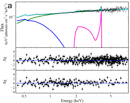
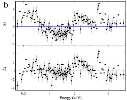
Figure 4: a: Co-added spectra of all Chandra images. The unfolded spectrum is shown to the best fit simple model with the relativistic line, soft disk component and power-law shown in magenta, blue and green respectively. The residuals to this model are shown in units of 1$\sigma$ deviations in the middle panel. The bottom panel shows the residuals after rebinned the data for display purposes. b: Top panel shows the residuals to a simple power-law and the bottom panel shows similar residuals after the addition of a DISKBB component.

Extended Data Fig. 4 (a) shows the time-averaged Chandra data fit with the baseline-simple model. This results in an excellent fit with ${\chi^{2}}/\nu=410.4/408=1.006$. The relativistic line at $E_{\rm RelLine}=6.49^{+0.05}_{-0.04}$$\rm\thinspace keV$ returns a broken emissivity profile with $Q_{\rm in}=7.2^{+0.4}_{-0.9}$ and $Q_{\rm out}<2.3$. Recall that broken emissivity profiles similar to the one found here is naturally expected when one suspects the black hole to be rapidly rotating and the corona to be compact[24, 7, 8]. The power-law index is found to be $1.69^{+0.02}_{-0.04}$ and the spin is constrained to

$$a=0.82^{+0.05}_{-0.09}~{}{\rm(90\%~{}confidence).}$$

Figure 2 in the main manuscript shows the ratio to this model after setting the normalisation of the disk and relativistic line component to zero, in order to highlight the contribution from these components. We also show in Extended Data Fig. 4 (b), the residuals to a single power-law before (top; ${\chi^{2}}/\nu=782.0/416=1.88)$ and after the addition of a DISKBB component (bottom; ${\chi^{2}}/\nu=546.3/414=1.32$). An equally good fit can be achieved with the addition of a narrow (1 eV) Gaussian at 6.4$\rm\thinspace keV$ together with the relativistic line now having $Q_{\rm out}=3$ (${\chi^{2}}/\nu=411.9/408=1.01$), and the spin value remains unchanged.

4.1.2 Baseline-reflection:

As a final step in our assessment of the robustness of our results based on the Chandra data alone, we again replace the phenomenological combination of components described above with REFLIONX convolved with RelConv. A narrow (1ev) Gaussian is again added at 6.4$\rm\thinspace keV$ and we use the broken emissivity profile with $Q_{out}=3$, as described above. Extended Data Fig. 5 (a) shows the fit to the time-averaged data and the right panel shows the extrapolated model. This model self-consistently accounts for the broad iron line and the soft-excess seen in this $z=0.658$ quasar, in a manner similar to the canonical recipe for nearby sources. The best fit (${\chi^{2}}/\nu=439.6/409=1.07$) again yields constraints on the spin which are consistent with all others presented in this work, i.e.

$$a=0.90^{+0.07}_{-0.15}~{}({\rm 3\sigma~{}confidence).}$$

We show the confidence contour for this model in Extended Data Fig. 3 (panel c; magenta contour). Extended Data Table 2 shows the parameters for this final model. As opposed to the phenomenological model described above, the additional narrow Gaussian at 6.4$\rm\thinspace keV$ is moderately statistically significant ($\Delta{\chi^{2}}=-6.5$ for one more degree of freedom) when using the physically motivated model. As such, it appears that the narrow feature at 6.4$\rm\thinspace keV$ is indeed due to a combination of emission from distant materials as well as from the outer regions of the accretion disk.

4.2 Additional XMM-Newton data:

4.2.1 Baseline-simple:

We now also consider our recent observation of RX J1131-1231 with XMM-Newton. A simple absorbed powerlaw model does not adequately describe the 0.3-10$\rm\thinspace keV$ range of the XMM-Newton EPIC-PN spectrum, with ${\chi^{2}}/\nu=982.5/858=1.15$ (see Extended Data Fig. 6). Adding a disk component similar to the Baseline-simple model improves the fit significantly ($\Delta{\chi^{2}}/\Delta\nu=65/2$) and an F-test shows that this extra component is required at greater than the $7\sigma$ level of confidence (F-test false alarm probability of $2\times 10^{-13}$). The relatively high effective area of XMM-Newton at energies greater than 5$\rm\thinspace keV$ also allows for the clear detection of a break in the continuum. Indeed by allowing the powerlaw to break, we find ${\chi^{2}}/\nu=899.9/854=1.05$, an improvement of $\Delta{\chi^{2}}/\Delta\nu=17.7/2$ (F-test false alarm probability of $2.5\times 10^{-4}$) over the fit without a break. Finally, the addition of a narrow Gaussian at $6.48^{+0.04}_{-0.03}$$\rm\thinspace keV$ (rest frame) yields a best fit of ${\chi^{2}}/\nu=862.4/852=1.01$ ( $\Delta{\chi^{2}}/\Delta\nu=37.5/2$; F-test false alarm probability of $1.3\times 10^{-8}$) for this phenomenological combination of components. This final model suggests the presence of a soft excess which can again be characterised by a DISKBB component with $kT=0.22\pm 0.03\hbox{$\rm\thinspace keV$}$, a powerlaw with an index $\Gamma=1.83^{+0.07}_{-0.03}$ up to a break at $E_{\rm break}=5.5^{+0.5}_{-2.2}\hbox{$\rm\thinspace keV$}$, at which point the continuum hardens to $\Gamma=1.28^{+0.33}_{-0.19}$. We show in Fig. 2 of the main manuscript the ratio to this $\Gamma=1.83$ powerlaw.

Within the reflection-paradigm, this combination of a hardening at $\sim 10\hbox{$\rm\thinspace keV$}$ (rest frame) together with a soft excess below $\sim 2\hbox{$\rm\thinspace keV$}$ can be characterised as the beginning of the Compton hump and the blending of soft emission lines, respectively. To our knowledge, this is the first clear detection of a break associated with a Compton hump in a moderate-z quasar. In the following subsection, we proceed by modelling this spectrum within the context of relativistic reflection.

4.2.2 Baseline-reflection:

We replace the phenomenological DISKBB component as well as the broken powerlaw with the Baseline-reflection model together with a narrow Gaussian (see Extended Data Fig. 6; b). This model is detailed in Extended Data Table 2. With a best fit of ${\chi^{2}}/\nu=849.4/849=1.000$, it is clear that this self-consistent description provides a quality of fit that significantly outperforms even that of the phenomenological combination presented above.

We show in Extended Data Fig. 3 (panel c; green) the confidence range for the spin as obtained from the XMM-Newton data alone. The spin found here of

$$a=0.64^{+0.33}_{-0.14}~{}({\rm 3\sigma~{}confidence),}$$

is again consistent with the range found during our analysis of the Chandra data.

It is clear from Extended Data Table 2 and Extended Data Figs. 5 and 6, that the ratio of the reflected flux to the powerlaw flux (the reflection fraction) is lower during the XMM-Newton observation, but the overall flux is higher. This trend of decreasing reflection fraction with increasing flux is often observed[15] in local AGN and within the reflection/light-bending interpretation[16] involves a corona whose height above the accretion disk is changing. In this scenario, a corona that is relatively close (a few ${\it r}_{\rm g}$s) to the black hole will have more of its emission bent towards the disk, decreasing the fraction of the coronal emission that escapes to the observer, and thus increasing the observed reflection fraction. On the other hand, if the corona is further from the black hole so that its emission can be better characterised as being isotropic, then the total flux illuminating the disk decreases (more flux escapes to the observer) and so does the reflection fraction. Importantly, the behaviour seen here is not only fully consistent with the expectations of gravitational light-bending, but it also requires a system having a high spin, consistent with the value reported in this work. Similar behaviour has been reported for a number of AGN, most famously 1H0707-495[24] and MCG -6-30-15 [15] as well as stellar mass black holes[2].

4.3 Joint XMM-Newton and Chandra fit with Baseline-reflection model:

It is clear from Extended Data Table 2 that, where the parameters are not expected to vary between observations, i.e. inclination, column density, and spin, the XMM-Newton observation yields consistent parameters to those obtained from the time-averaged Chandra data. In order to optimise the S/N and obtain a final estimate of the spin parameter of RX J1131-1231, we proceed by fitting both data sets simultaneously with the Baseline-reflection model, with the inclination, column density and spin tied between them. Extended Data Table 2 also details the various parameters for this final, joint fit and Figure 3 in the main manuscript (duplicated in Extended Data Fig. 3; panel c; black) shows the confidence contour obtained for the spin where we find a value of

$$a=0.87^{+0.08}_{-0.15}~{}({\rm 3\sigma~{}confidence),}$$

based on the combined Chandra and XMM-Newton data.

5 No Evidence for Complex Absorption in RX J1131-1231:

To this point, we have based our modelling on the reflection paradigm and followed the well established methodology that has been applied to many local Seyferts. We note, however, that $\sim 50\%$ of these Seyferts[17] and a similar number of quasars[11] also display evidence for absorption by partially ionised, optically-thin material local to the accretion flow (“warm” absorbers; WAs).

Indeed, the canonical Seyfert galaxy, MCG-6-30-15, displays one of the most prominent relativistic lines known, and its X-ray spectrum also requires the presence of multiple absorption zones. Early spin measurements of MCG-6-30-15 (e.g. ref[8]) often strictly focused on data $\gtrsim 2$$\rm\thinspace keV$, as the main effect of these warm absorbers are below this energy (e.g. ref[18]), notably the two strong edges of O VII and O VIII at $\sim 0.74$$\rm\thinspace keV$ and $\sim 0.87$$\rm\thinspace keV$, respectively [19] (note that for RX J1131-1231 at $z=0.658$, this restricts the bulk effect of any possible WA to energies $\lesssim 0.5$$\rm\thinspace keV$). However, subsequent detailed analyses accounting for the multizone warm absorber present in this source still obtained consistent spin measurements[15, 12, 20] and concluded that the relativistic iron line is robust to the precise details of the WA (e.g. [21]). Nonetheless, the presence of such a component in half of all quasars prompted us to investigate whether the residuals seen in RX J1131-1231 could be explained by WAs, and what effect the presence of a putative WA will have on our ability to constrain the spin of the black hole.

5.1 Partially Ionised Absorption:

5.1.1 Phenomenological modeling:

We start by fitting the co-added spectra of Images-B and C with a model describing partially covering absorption by a partially ionised medium (zxipcf in XSPEC; ref[22]). The WA is characterised with an ionisation parameter $\xi_{\rm wa}=L/nr^{2}\hbox{$\rm\thinspace erg~{}cm~{}s^{-1}$}$, where $L$ is the ionising X-ray luminosity ($\rm\thinspace erg~{}s^{-1}$), $n$ the gas density (${\rm cm^{-3}}$), and $r$ is the distance in centimeters between the source of ionising X-rays and the absorbing gas. The model also includes the covering fraction ($cf$) which defines the fraction of the source which is covered by the absorbing gas with a column density $N_{\rm H;wa}$, while the remaining (1-$cf$) flux from the source escapes directly to the observer. We initially allow the ionisation parameter, column density and covering fraction of zxipcf to be free, and apply this to a simple absorbed power-law model. In XSPEC terminology this model reads phabs$\times$ (zphabs $\times$(zxipcf $\times$ (zpowerlaw))).

This model provided a goodness of fit equal to that of the power-law+DISKBB combination for both images (${\chi^{2}}_{\rm B}/\nu_{\rm B}=426.1/355=1.20$ and ${\chi^{2}}_{\rm C}/\nu_{\rm C}=263.6/247=1.07$ for Images-B and C respectively), meaning that it can account for the “soft-excess” to the same degree as the previous model using DISKBB. However, like the fit with a DISKBB, this model still cannot account for the residuals above $\sim 2$$\rm\thinspace keV$. Adding a Gaussian, constrained to lie in the Fe K-shell energy range (6.4-6.97$\rm\thinspace keV$ local frame), to Image-B does not improve the fit; however, upon lifting this constraint we obtain an improvement (${\chi^{2}}_{\rm B}/\nu_{\rm B}=414.0/352=1.18$). The Gaussian line has a centroid energy of $E_{\rm Gaussian}=3.61^{+0.26}_{-0.24}$$\rm\thinspace keV$ (local frame) and a width of $\sigma=710^{+370}_{-570}$$\rm\thinspace eV$. It is clear that such a broad line, with a centroid energy much lower than the 6.4$\rm\thinspace keV$ expected for neutral iron is a rather unphysical combination which is artificially mimicking a broad, relativistic line. Alternative scenarios such as Compton broadening aimed at explaining broad lines of this magnitude have been shown to not be a viable alternative in Seyfert galaxies[29]. As such, we replace the Gaussian with RelLine and constrain the energy to 6.4-6.97$\rm\thinspace keV$ as per usual. This model, with a WA, provides a better fit (${\chi^{2}}_{\rm B}/\nu_{\rm B}=407.2/349=1.17$), and most importantly, models the residuals in a physically motivated manner. We note that adding a second zone does not improve the fits. Focusing on Image-C, we find that while the addition of a Gaussian does improve the fit (${\chi^{2}}_{\rm C}/\nu_{\rm C}=241.0/244=0.99$), it is not statistically significant. Replacing this Gaussian with RelLine does remove clear systematic residuals and indeed increases the goodness of fit to ${\chi^{2}}_{\rm C}/\nu_{\rm C}=234.1/241$ ($\chi^{2}_{\nu}=0.97$).

The ionisation parameter of the putative WA is not well constrained for either image, with both cases resulting in upper limits of ${\rm log_{10}}\xi\lesssim 1.5$. It is clear that the WA is having the same affect as the phenomenological DISKBB model. However, the spin obtained via the relativistic line alone for Images-B and C are consistent with all other results presented here ($a_{\rm B}=0.89^{+0.02}_{-0.09}$ and $a_{\rm C}=0.8^{+0.09}_{-0.06}$ at the 90% confidence), and most importantly is still constrained to be high.

5.1.2 Baseline-reflection:

As a broad relativistic Fe-$K\alpha$ line is naturally accompanied by other emission at lower energies, which can self-consistently account for the soft-excess, we proceed by reverting back to our baseline-reflection model (as detailed on Extended Data Table 1) in order to model the residuals above $\sim 2$$\rm\thinspace keV$(observed frame) in both images. However, we now include an additional WA in order to investigate any possible effect on the results obtained with this model.

The addition of zxipcf to the Baseline-reflection model for the co-added Image-B data improves the quality of the fit by $\Delta{\chi^{2}}_{\rm B}/\Delta\nu_{\rm B}=-5.2/-3$ (final ${\chi^{2}}_{\rm B}/\nu_{\rm B}=402.4/348=1.16$), i.e., this extra component is not statistically significant. Nonetheless, we note that this fit to Image-B yields $N_{\rm H;wa;B}=(1.4^{+5.0}_{-0.8})\times 10^{22}\hbox{$\rm\thinspace cm^{-2}$}$, ${\rm log_{10}}\xi_{\rm wa;B}<2.1$ and $cf=0.2^{+0.3}_{-0.1}$. All other parameters stay the same as those presented in Table S1, within the errors. As the addition of this extra component over the baseline-reflection model is not statistically significant, we also tried fixing ${\rm log_{10}}\xi_{\rm wa;B}=2$, typical of both Seyferts like MCG-6-30-15 as well as Quasars such as PG 1309+355 (ref[23]). Again the improvement over a model without such absorption is barely significant at $\Delta{\chi^{2}}_{\rm B}/\Delta\nu_{\rm B}=-3.1/-2$; nonetheless, this fit again gives a low covering fraction ($cf<0.27$) and the constraint on the spin remains essentially unchanged ($a=0.91\pm 0.05$) from that reported on Extended Data Tables 1. Freezing ${\rm log_{10}}\xi_{\rm wa;B}=3$ or 1 does not change this conclusion nor does the addition of a second WA.

Adding a similar absorber to the baseline-reflection model for Image-C does not provide any improvement over that reported on Extended Data Table 1 and none of the WA parameters are constrained. We thus proceed by again freezing the ionisation to ${\rm log_{10}}\xi_{\rm wa;B}=2$ and setting the column density to $N_{\rm H;wa;C}=1\times 10^{22}\hbox{$\rm\thinspace cm^{-2}$}$ so as to obtain a rough limit on any potential covering fraction. This imposed WA provides a fit that is statistically similar to that shown in Extended Data Table 1 and sets a limit on the covering fraction of $cf\leq 0.12$. Again the spin remains unchanged.

We have also investigated the addition of a WA to the baseline-reflection model used in the time-resolved spectral analyses presented in § 3. We initially allowed the column density and covering fraction to vary between epochs but kept the ionisation parameter frozen at ${\rm log_{10}}\xi_{\rm wa}=2$. This did not improve the fits. Neither did freezing the ionisation at ${\rm log_{10}}\xi_{\rm wa}=3$, or allowing it to vary between epochs. In fact, the additional 54 or 81 free parameters, depending on whether ${\rm log_{10}}\xi_{\rm wa}$ was frozen or not, made the overall reduced ${\chi^{2}}$ worse than that without this extra component. It is clear that the addition of a WA does not improve the quality of the fits nor does it affect the values for the spin obtained here. We therefore conclude that RX J1131-1231 does not require the presence of a WA on top of the self-consistent baseline-reflection model.

5.2 Neutral Absorption:

We have also investigated the use of multiple neutral, partially covering absorption components, in addition to the fully covering neutral absorption included in all models, with the ZPCFABS model within XSPEC. Initially we restrict our consideration to Compton-thin absorption. First, we add an additional partially covering neutral absorber to the relativistic reflection model considered previously for the joint Chandra and XMM-Newton dataset. We obtain a best fit commensurate with that reported on Extended Data Table 2, with ${\chi^{2}}/\nu=1279.2/1256=1.02$ and most importantly, a spin parameter tightly constrained to $a=0.75^{+0.06}_{-0.09}$ ($3\sigma$); statistically similar to that reported on Extended Data Table 2. Second, we attempt to construct absorption-dominated models, but find that it is not possible to reproduce either the combined Chandra or the XMM-Newton data solely using reasonable combinations of such models, i.e. without any contribution from relativistic reflection. For the Chandra data, residuals associated with the broad iron line still persist, and it is not possible to account for the spectral curvature above $\sim$5 $\rm\thinspace keV$ in the XMM-Newton data.

Finally, we relax the requirement that the absorbers are Compton-thin. However, we find this only influences the fit to the XMM-Newton data, where we find that a partially-covering ($cf=0.27^{+0.12}_{-0.11}$), Compton-thick absorber (${\it N}_{\rm H}$ = $1.68^{+1.75}_{-0.72}\times 10^{24}\hbox{$\rm\thinspace cm^{-2}$}$) can successfully account for the high-energy excess in the XMM-Newton data. We therefore also include in this model a cold ($\xi=1$), unblurred REFLIONX component aimed at simulating reprocessed emission from Compton-thick material far from the black hole. Nevertheless, when this model is applied to the joint XMM-Newton and Chandra dataset, with the partially covering absorber allowed to vary between the XMM-Newton and Chandra data, despite a visibly good fit to the XMM-Newton data above $\sim 5$$\rm\thinspace keV$ now being obtained this model still provides a worse fit ($\Delta{\chi^{2}}=54.7$) than the Baseline-reflection model, and systematic residuals persist in the Chandra data between $\sim$1–5 $\rm\thinspace keV$. Although the best fit absorber for the Chandra data remains Compton-thin (${\it N}_{\rm H}$ = $8.40^{+1.14}_{-0.97}\times 10^{22}\hbox{$\rm\thinspace cm^{-2}$}$), a similar covering fraction is inferred ($cf=0.31\pm 0.03$). Given the known size of the X-ray emitting region ($\sim$10 ${\it r}_{\rm g}$), determined independently by X-ray microlensing[20], such small covering fractions require a highly fine-tuned and ad-hoc geometry for the absorbing cloud. Furthermore, we stress that a scenario in which the spectral features are formed by absorprion/reprocessing by large, distant, distributed structures is also strongly at odds with the known size of the X-ray source.

Supplementary Figures

Supplementary Tables

Table 1 — Model summary for the co-added spectra of Images-B and C.

	Baseline-simple		Baseline-reflection
parameters	image B	image C	image B	image C
$N_{\rm H}(z=0.658)$ ($\times 10^{21}\hbox{$\rm\thinspace cm^{-2}$}$)	$1.4^{+0.8}_{-0.4}$	$<2$	$1.1^{+0.3}_{-0.5}$	$<0.8$
$\Gamma$	$1.65^{+0.03}_{-0.02}$	$1.71^{+0.06}_{-0.04}$	$1.62^{+0.15}_{-0.11}$	$1.55^{+0.13}_{-0.15}$
$N_{\rm power-law}$ ($\times 10^{-4}$)	$2.6\pm 0.1$	$0.85\pm 0.08$	$<1.19$ •	$0.38^{+0.29}_{-0.14}$
$T_{\rm Diskbb}$ ($\rm\thinspace keV$)	$0.12\pm 0.01$	$0.15^{+0.09}_{-0.04}$	• — •	—
$N_{\rm Diskbb}$	$200^{+270}_{-140}$	$14^{+90}_{-9}$	• — •	—
$E_{\rm RelLine}$ ($\rm\thinspace keV$)	$6.43^{+0.05}$	$6.49\pm 0.06$	• — •	—
$Q_{\rm in}$	$7.8^{+0.7}_{-1.9}$	$6.5^{+0.5}_{-1.1}$	• $6.1^{+0.4}_{-0.7}$	$7.0^{+0.9}_{-1.8}$
$Q_{\rm out}$	$<2.7$	$<2.3$	$<3.7$	$<8$
Inclination	$<13$	$<16$	$26^{+8}_{-14}$	$<27$
$N_{\rm RelLine}$ ($\times 10^{-6}$)	$7.0^{+2.5}_{-1.7}$	$3.3.0^{+1.6}_{-1.2}$	• — •	—
$N_{\rm ReflionX}$ ($\times 10^{-8}$)	—	—	$6.9^{+3.3}_{-3.5}$	$0.45^{+0.05}_{-0.03}$
$\xi$ ($\rm\thinspace erg~{}cm~{}s^{-1}$)	—	—	$623^{+230}_{-210}$	$1290^{+890}_{-870}$
${\rm f_{\rm reflect}/f_{\rm illum}}$ $(0.1-10)$$\rm\thinspace keV$	—	—	$3.6\pm 2.5$	$1.4\pm 1.2$
${\rm f_{\rm reflect}/f_{\rm illum}}$ $(0.1-100)$$\rm\thinspace keV$	—	—	$2.6\pm 2.0$	$0.9\pm 0.6$
Spin ($a={\rm Jc/GM^{2}}$)	$0.73\pm 0.04$	$0.79^{+0.11}_{-0.07}$	$0.92^{+0.04}_{-0.06}$	$0.80^{+0.08}_{-0.06}$
${\chi^{2}}/\nu$	$393.9/350$	$231.0/242$	•$407.5/351$	$238.6/243$

Notes: ^a Rest frame energy constrained between 6.4-6.97$\rm\thinspace keV$. ^b Value for the outer emissivity constrained to be $>2$ with a break radius frozen at 10${\it r}_{\rm g}$. All models include a fixed Galactic absorption of $N_{\rm H}(z=0)=0.36\times 10^{21}\hbox{$\rm\thinspace cm^{-2}$}$. ^c Reflection fraction defined as the ratio of the reflected to the illuminating continuum in the given energy band. All errors are 90% confidence on one parameter

Table 2 —  Model summary for the time-averaged Chandra spectrum of RX J1131-1231 as well as the XMM-Newton EPIC-PN data using Baseline-reflection.

	Individual		Joint
parameter	Chandra	XMM-Newton	Chandra	XMM-Newton
$N_{\rm H}(z=0.658$) ($\times 10^{21}\hbox{$\rm\thinspace cm^{-2}$}$)	$0.8^{+0.3}_{-0.5}$	$1.1^{+0.3}_{-0.4}$	$1.07^{+0.26}_{-0.16}$
$\Gamma$	$1.59\pm 0.08$	$2.02\pm 0.04$	$1.64^{+0.06}_{-0.05}$	$2.02^{+0.04}_{-0.03}$
$N_{\rm power-law}$ ($\times 10^{-5}$)	$6.3^{+2.5}_{-2.1}$	$187^{+5}_{-4}$	$9.4^{+2.9}_{-2.3}$	$187\pm 4$
$Q_{\rm in}$	$6.0^{+0.8}_{-0.4}$	$>5.4$	$>5.9$	$5.0^{+1.4}_{-1.5}$
$Q_{\rm out}$	$<2.4$	$3.3^{+1.1}_{-0.7}$	$2.9^{+0.2}_{-0.8}$	$3.3^{+1.0}_{-1.3}$
$R_{\rm break}$ ($r_{\rm G}={\rm GM/c^{2}}$)	10(f)	$6^{+4}_{-1}$	$5.9^{+3.0}_{-1.7}$	$<20$
Inclination	$20^{+6}_{-7}$	$<17$	$15^{+9}_{-15}$
$N_{\rm ReflionX}$ ($\times 10^{-8}$)	$3.0^{+1.2}_{-1.0}$	$75\pm 34$	$2.8^{+0.6}_{-1.3}$	$78^{+44}_{-16}$
$\xi(\rm\hbox{$\rm\thinspace erg~{}cm~{}s^{-1}$})$	$725^{+286}_{-118}$	$99^{+15}_{-37}$	$612^{+195}_{-92}$	$98^{+16}_{-4}$
${\rm f_{\rm reflect}/f_{\rm illum}}$ $(0.1-10)$$\rm\thinspace keV$	$2.3\pm 1.2$	$0.47\pm 0.15$
${\rm f_{\rm reflect}/f_{\rm illum}}$ $(0.1-100)$$\rm\thinspace keV$	$1.65\pm 0.95$	$0.53\pm 0.13$
Spin ($a={\rm Jc/GM^{2}}$)	$0.90^{+0.07}_{-0.15}$	$0.64^{+0.33}_{-0.14}$	$a=0.87^{+0.08}_{-0.15}$
${\chi^{2}}/\nu$	$439.6/409$	$849.4/849$	$1296.1/1260$

Notes: ^a Value for the outer emissivity constrained to be $>2$. (f) denotes frozen values. ^b Reflection fraction defined as the ratio of the reflected to the illuminating continuum in the given energy band. All models include a fixed Galactic absorption of $N_{\rm H}(z=0)=0.36\times 10^{21}\hbox{$\rm\thinspace cm^{-2}$}$. ^cAll errors are 90% confidence on one parameter except for the spin where we show the $3\sigma$ limit.

References

- [1] Gebhardt, K. et al. A Relationship between Nuclear Black Hole Mass and Galaxy Velocity Dispersion. Astrophys. J. 539, L13–L16 (2000). arXiv:astro-ph/0006289.
- [2] Berti, E. & Volonteri, M. Cosmological Black Hole Spin Evolution by Mergers and Accretion. Astrophys. J. 684, 822–828 (2008). 0802.0025.
- [3] Fanidakis, N. et al. Grand unification of AGN activity in the CDM cosmology. Mon. Not. R. Astron. Soc. 410, 53–74 (2011). 0911.1128.
- [4] Volonteri, M., Sikora, M., Lasota, J.-P. & Merloni, A. The Evolution of Active Galactic Nuclei and their Spins. Astrophys. J. 775, 94 (2013). 1210.1025.
- [5] King, A. R. & Pringle, J. E. Growing supermassive black holes by chaotic accretion. Mon. Not. R. Astron. Soc. 373, L90–L92 (2006). arXiv:astro-ph/0609598.
- [6] Risaliti, G. et al. A rapidly spinning supermassive black hole at the centre of NGC1365. Nature 494, 449–451 (2013). 1302.7002.
- [7] Ross, R. R. & Fabian, A. C. The effects of photoionization on X-ray reflection spectra in active galactic nuclei. Mon. Not. R. Astron. Soc. 261, 74–82 (1993).
- [8] Tanaka, Y. et al. Gravitationally redshifted emission implying an accretion disk and massive black hole in the active galaxy MCG-6-30-15. Nature 375, 659–661 (1995).
- [9] Crummy, J., Fabian, A. C., Gallo, L. & Ross, R. R. An explanation for the soft X-ray excess in active galactic nuclei. Mon. Not. R. Astron. Soc. 365, 1067–1081 (2006). arXiv:astro-ph/0511457.
- [10] Walton, D. J., Nardini, E., Fabian, A. C., Gallo, L. C. & Reis, R. C. Suzaku observations of ‘bare’ active galactic nuclei. Mon. Not. R. Astron. Soc. 428, 2901–2920 (2013). 1210.4593.
- [11] Porquet, D., Reeves, J. N., O’Brien, P. & Brinkmann, W. XMM-Newton EPIC observations of 21 low-redshift PG quasars. Astron. Astrophys. 422, 85–95 (2004). arXiv:astro-ph/0404385.
- [12] Piconcelli, E. et al. The XMM-Newton view of PG quasars. I. X-ray continuum and absorption. Astron. Astrophys. 432, 15–30 (2005). arXiv:astro-ph/0411051.
- [13] Jiménez-Bailón, E. et al. The XMM-Newton view of PG quasars. II. Properties of the Fe K_ line. Astron. Astrophys. 435, 449–457 (2005). arXiv:astro-ph/0501587.
- [14] Green, P. J. et al. A Full Year’s Chandra Exposure on Sloan Digital Sky Survey Quasars from the Chandra Multiwavelength Project. Astrophys. J. 690, 644–669 (2009). 0809.1058.
- [15] Pooley, D., Blackburne, J. A., Rappaport, S. & Schechter, P. L. X-Ray and Optical Flux Ratio Anomalies in Quadruply Lensed Quasars. I. Zooming in on Quasar Emission Regions. Astrophys. J. 661, 19–29 (2007). arXiv:astro-ph/0607655.
- [16] Chartas, G. et al. Revealing the Structure of an Accretion Disk through Energy-dependent X-Ray Microlensing. Astrophys. J. 757, 137 (2012). 1204.4480.
- [17] Gilli, R., Comastri, A. & Hasinger, G. The synthesis of the cosmic X-ray background in the Chandra and XMM-Newton era. Astron. Astrophys. 463, 79–96 (2007). arXiv:astro-ph/0610939.
- [18] Sluse, D., Hutsemékers, D., Courbin, F., Meylan, G. & Wambsganss, J. Microlensing of the broad line region in 17 lensed quasars. Astron. Astrophys. 544, A62 (2012). 1206.0731.
- [19] Sluse, D. et al. A quadruply imaged quasar with an optical Einstein ring candidate: 1RXS J113155.4-123155. Astron. Astrophys. 406, L43–L46 (2003). arXiv:astro-ph/0307345.
- [20] Dai, X. et al. The Sizes of the X-ray and Optical Emission Regions of RXJ 1131-1231. Astrophys. J. 709, 278–285 (2010). 0906.4342.
- [21] Reis, R. C. & Miller, J. M. On the Size and Location of the X-Ray Emitting Coronae around Black Holes. Astrophys. J. 769, L7 (2013). 1304.4947.
- [22] Miller, J. M. et al. On Relativistic Disk Spectroscopy in Compact Objects with X-ray CCD Cameras. Astrophys. J. 724, 1441–1455 (2010). 1009.4391.
- [23] Reynolds, C. S. Measuring Black Hole Spin using X-ray Reflection Spectroscopy. ArXiv e-prints (2013). 1302.3260.
- [24] Fabian, A. C. et al. Broad line emission from iron K- and L-shell transitions in the active galaxy 1H0707-495. Nature 459, 540–542 (2009).
- [25] Miller, J. M. Relativistic X-Ray Lines from the Inner Accretion Disks Around Black Holes. Ann. Rev. Astron. Astrophys. 45, 441–479 (2007). 0705.0540.
- [26] Schmoll, S. et al. Constraining the Spin of the Black Hole in Fairall 9 with Suzaku. Astrophys. J. 703, 2171–2176 (2009). 0908.0013.
- [27] Haardt, F. & Maraschi, L. A two-phase model for the X-ray emission from Seyfert galaxies. Astrophys. J. 380, L51–L54 (1991).
- [28] Falcke, H. & Markoff, S. The jet model for Sgr A*: Radio and X-ray spectrum. Astron. Astrophys. 362, 113–118 (2000). arXiv:astro-ph/0102186.
- [29] Walton, D. J., Reis, R. C., Cackett, E. M., Fabian, A. C. & Miller, J. M. The similarity of broad iron lines in X-ray binaries and active galactic nuclei. Mon. Not. R. Astron. Soc. 422, 2510–2531 (2012). 1202.5193.
- [30] Reynolds, C. S. & Fabian, A. C. Broad Iron-K Emission Lines as a Diagnostic of Black Hole Spin. Astrophys. J. 675, 1048–1056 (2008). 0711.4158.

References

- [1] Chartas, G., Kochanek, C. S., Dai, X., Poindexter, S. & Garmire, G. X-Ray Microlensing in RXJ1131-1231 and HE1104-1805. Astrophys. J. 693, 174–185 (2009).
- [2] Fruscione, A. et al. CIAO: Chandra’s data analysis system. In Society of Photo-Optical Instrumentation Engineers (SPIE) Conference Series, vol. 6270 of Society of Photo-Optical Instrumentation Engineers (SPIE) Conference Series (2006).
- [3] Tsunemi, H. et al. Improvement of the Spatial Resolution of the ACIS Using Split-Pixel Events. Astrophys. J. 554, 496–504 (2001).
- [4] Wang, J. et al. A Deep Chandra ACIS Study of NGC 4151. I. The X-ray Morphology of the 3 kpc Diameter Circum-nuclear Region and Relation to the Cold Interstellar Medium. Astrophys. J. 729, 75 (2011).
- [5] Davis, J. E. Event Pileup in Charge-coupled Devices. Astrophys. J. 562, 575–582 (2001).
- [6] Russell, H. R. et al. The X-ray luminous cluster underlying the bright radio-quiet quasar H1821+643. Mon. Not. R. Astron. Soc. 402, 1561–1579 (2010).
- [7] Dauser, T., Wilms, J., Reynolds, C. S. & Brenneman, L. W. Broad emission lines for a negatively spinning black hole. Mon. Not. R. Astron. Soc. 409, 1534–1540 (2010).
- [8] Dickey, J. M. & Lockman, F. J. H I in the Galaxy. Ann. Rev. Astron. Astrophys. 28, 215–261 (1990).
- [9] Balucinska-Church, M. & McCammon, D. Photoelectric absorption cross sections with variable abundances. Astrophys. J. 400, 699–+ (1992).
- [10] Anders, E. & Grevesse, N. Abundances of the elements - Meteoritic and solar. Geochimica et Cosmochimica Acta 53, 197–214 (1989).
- [11] Tewes, M. et al. COSMOGRAIL: the COSmological MOnitoring of GRAvItational Lenses. XIII. Time delays and 9-yr optical monitoring of the lensed quasar RX J1131-1231. Astron. Astrophys. 556, A22 (2013).
Supplementary Information

References

- [1]
- [2] Reis, R. C. et al. Evidence of Light-bending Effects and Its Implication for Spectral State Transitions. Astrophys. J. 763, 48 (2013).
- [3] Brenneman, L. W. et al. The Spin of the Supermassive Black Hole in NGC 3783. Astrophys. J. 736, 103 (2011).
- [4] Reis, R. C. et al. X-Ray Spectral Variability in NGC 3783. Astrophys. J. 745, 93 (2012).
- [5] Popović, L. Č., Mediavilla, E. G. & Muñoz, J. A. The influence of microlensing on spectral line shapes generated by a relativistic accretion disc. Astron. Astrophys. 378, 295–301 (2001).
- [6] Abajas, C., Mediavilla, E., Muñoz, J. A., Popović, L. Č. & Oscoz, A. The Influence of Gravitational Microlensing on the Broad Emission Lines of Quasars. Astrophys. J. 576, 640–652 (2002).
- [7] Fabian, A. C. et al. On the determination of the spin of the black hole in Cyg X-1 from X-ray reflection spectra. Mon. Not. R. Astron. Soc. 3135 (2012).
- [8] Wilkins, D. R. & Fabian, A. C. Determination of the X-ray reflection emissivity profile of 1H 0707-495. Mon. Not. R. Astron. Soc. 414, 1269–1277 (2011).
- [9] Ross, R. R. & Fabian, A. C. A comprehensive range of X-ray ionized-reflection models. Mon. Not. R. Astron. Soc. 358, 211–216 (2005).
- [10] Fabian, A. C. & Vaughan, S. The iron line in MCG-6-30-15 from XMM-Newton: evidence for gravitational light bending? Mon. Not. R. Astron. Soc. 340, L28–L32 (2003).
- [11] Fabian, A. C. et al. A long hard look at MCG-6-30-15 with XMM-Newton. Mon. Not. R. Astron. Soc. 335, L1–L5 (2002).
- [12] Brenneman, L. W. & Reynolds, C. S. Constraining Black Hole Spin via X-Ray Spectroscopy. Astrophys. J. 652, 1028–1043 (2006).
- [13] Hamann, F. & Ferland, G. The Chemical Evolution of QSOs and the Implications for Cosmology and Galaxy Formation. Astrophys. J. 418, 11 (1993).
- [14] Iwamuro, F. et al. Fe II/Mg II Emission-Line Ratios of QSOs within 0 z 5.3. Astrophys. J. 565, 63–77 (2002).
- [15] Vaughan, S. & Fabian, A. C. A long hard look at MCG-6-30-15 with XMM-Newton- II. Detailed EPIC analysis and modelling. Mon. Not. R. Astron. Soc. 348, 1415–1438 (2004).
- [16] Miniutti, G. & Fabian, A. C. A light bending model for the X-ray temporal and spectral properties of accreting black holes. Mon. Not. R. Astron. Soc. 349, 1435–1448 (2004).
- [17] Reynolds, C. S. An X-ray spectral study of 24 type 1 active galactic nuclei. Mon. Not. R. Astron. Soc. 286, 513–537 (1997).
- [18] Lee, J. C. et al. Revealing the Dusty Warm Absorber in MCG -6-30-15 with the Chandra High-Energy Transmission Grating. Astrophys. J. 554, L13–L17 (2001).
- [19] Fabian, A. C. et al. ASCA observations of the warm absorber in MCG-6-30-15: The discovery of a change in column density. Publ. Astron. Soc. Jap. 46, L59–L63 (1994).
- [20] Chiang, C.-Y. & Fabian, A. C. Modelling the broad-band spectra of MCG-6-30-15 with a relativistic reflection model. Mon. Not. R. Astron. Soc. 414, 2345–2353 (2011).
- [21] Young, A. J. et al. A Chandra HETGS Spectral Study of the Iron K Bandpass in MCG -6-30-15: A Narrow View of the Broad Iron Line. Astrophys. J. 631, 733–740 (2005).
- [22] Reeves, J. et al. On why the iron K-shell absorption in AGN is not a signature of the local warm/hot intergalactic medium. Mon. Not. R. Astron. Soc. 385, L108–L112 (2008).
- [23] Ashton, C. E. et al. XMM-Newton observations of warm absorbers in PG quasars. Mon. Not. R. Astron. Soc. 355, 73–81 (2004).