Spin susceptibility of two-dimensional transition metal dichalcogenides

Abstract

We have obtained analytical expressions for the $q$-dependent static spin susceptibility of monolayer transition metal dichalcogenides, considering both the electron-doped and hole-doped cases. Our results are applied to calculate spin-related physical observables of monolayer MoS₂, focusing especially on in-plane/out-of-plane anisotropies. We find that the hole-mediated RKKY exchange interaction for in-plane impurity-spin components decays with the power law $R^{-5/2}$ as a function of distance $R$, which deviates from the $R^{-2}$ power law normally exhibited by a two-dimensional Fermi liquid. In contrast, the out-of-plane spin response shows the familiar $R^{-2}$ long-range behavior. We also use the spin susceptibility to define a collective $g$-factor for hole-doped MoS₂ systems and discuss its density-dependent anisotropy.

I Introduction

The discovery of grapheneNovoselov et al. (2004); Castro Neto et al. (2009), a monolayer of carbon atoms arranged in a honeycomb lattice, and its intriguing physical properties has triggered a search for other materials that, like graphene, are intrinsically two-dimensional (2D). Despite its huge potential for applications in electronic devicesBolotin et al. (2008); Morozov et al. (2008); Han et al. (2007); Novoselov et al. (2012), there are seveal reasons to consider alternatives to graphene. An important motivation is provided by the fact that pristine graphene is a semimetal, i.e., its conduction and valence bands touch at the neutrality (Dirac) point. The absence of an energy gap creates difficulties for realizing graphene-based conventional semiconductor devicesAndo (2009). Furthermore, graphene has a very weak spin-orbit coupling (SOC)Min et al. (2006); Konschuh et al. (2010). Having a similar material with strong intrinsic SOC would open up possibilities for pursuing novel (e.g., magnet-less) spintronic applicationsŽutić et al. (2004).

Two-dimensional crystals of transition metal dichalcogenides have recently been identified as graphene-like materials that have very interesting properties and great promise for enabling electronic and spintronic applicationsWang et al. (2012); Xu et al. (2014). As a member of this materials class, monolayer MoS₂ has attracted a lot of attention recentlyRadisavljevic et al. (2011); Zeng et al. (2012); Cao et al. (2012). While bulk MoS₂ is an indirect-gap semiconductor, a monolayer is found to be semiconducting with a direct band gapMak et al. (2010); Xiao et al. (2012); Kormányos et al. (2013); Rostami et al. (2013); Cappelluti et al. (2013); Cheiwchanchamnangij et al. (2013). Monolayer MoS₂ has a honeycomb-lattice structure with Mo and S atoms located on different sublattices. This arrangement gives rise to a broken inversion symmetry, which in turn yields a relatively large band gap ($\sim\,$1.66 eV). Due to the relevant admixture of Mo $d$-orbitals, monolayer MoS₂ also has a strong SOC, rendering it a good candidate for spintronic applicationsNeal et al. (2013); Klinovaja and Loss (2013). Recent theoretical studies of MoS₂ have focused on the many-particle and collective response properties of its charge carriers. Plasmon dispersions and static screening have been investigated within the random phase approximationScholz et al. (2013). Other worksLu et al. (2013); Song and Dery (2013); Ochoa et al. (2013); Ochoa and Roldán (2013); Wang and Wu ; Yu and Wu have discussed the various spin-relaxation processes that can occur in MoS₂. Furthermore, the carrier-mediated exchange interaction between localized magnetic impurities has been calculatedParhizgar et al. (2013) within the framework of the RKKY mechanismRuderman and Kittel (1954); Kasuya (1956); Yosida (1957) and using first-principle methods Cheng et al. (2013); Mishra et al. (2013). A recent study Dolui et al. (2013) has systematically explored realistic strategies for achieving n-type and p-type doping in monolayer MoS₂.

Our work sheds new light on the spin response of 2D transition metal dichalcogenides. Analytical results for the wave-vector-dependent spin susceptibilityMoriya (1985); Yosida (1996) $\chi_{ij}({\bm{\mathrm{q}}})$ are obtained based on ${\bm{\mathrm{k}}}\cdot{\bm{\mathrm{p}}}$ model-Hamiltonian descriptionsXiao et al. (2012); Kormányos et al. (2013); Rostami et al. (2013). Physical consequences are discussed and illustrated using band-structure parameters for MoS₂. We reveal interesting features exhibited by carrier-mediated exchange interactions between local magnetic moments and Zeeman spin splitting as encoded in the electronic $g$-factor. The hole-doped material turns out to have particularly rich spin properties, whereas the electron-doped case shows behavior quite similar to that of ordinary 2D electron systems. Nevertheless, from a conceptual point of view, consideration of the electron-doped material is useful because it serves as an instructive testbed for understanding the interplay between extrinsic and intrinsic contributions to the spin response, where the former (latter) result from filled states in the conduction (valence) band. Thus the spin-response properties of monolayer transition metal dichalcogenides constitute an intriguing intermediate behavior between that exhibited by graphene and ordinary 2D electron systems realized in semiconductor heterostructures. Besides adding to the basic understanding of a new materials class, our results also suggest practical ways for electronic manipulation of its spin structure.

The remainder of this article is organized as follows. In Sec. II, we introduce the low-energy effective Hamiltonian that underpins our calculations and present a general expression for the spin-susceptibility tensor in terms of single-particle eigenstates and -energies. Analytical results for $\chi_{ij}({\bm{\mathrm{q}}})$ are presented in the subsequent two sections; for the electron-doped case in Sec. III and for the hole-doped case in Sec. IV. We discuss salient features of spin-related physical observables for the hole-doped system in Sec V. Section VI contains a summary of our results and conclusions. A detailed derivation of the basic expression for the spin susceptibility used in our work is provided in the Appendix.

II Details of theoretical approach

II.1 Model-Hamiltonian description

As our formal basis for the calculation of the spin susceptibility, we adopt the low-energy effective Hamiltonian for monolayer transition metal dichalcogenides derived in Ref. Xiao et al., 2012 (see also Refs. Kormányos et al., 2013; Rostami et al., 2013). To lowest order in the in-plane wave vector ${\bm{\mathrm{k}}}=(k_{x},k_{y})$, it reads 

$$H^{\tau}_{0}=at(\tau k_{x}{\hat{\sigma}_{x}}+k_{y}\hat{\sigma}_{y})\otimes\openone+\frac{\Delta}{2}\hat{\sigma}_{z}\otimes\openone-\frac{\lambda\tau}{2}\left(\hat{\sigma}_{z}-\openone\right)\otimes\hat{s}_{z}~{}.$$ (1)

The valley index $\tau=\pm 1$ distinguishes electronic excitations at the two nonequivalent high-symmetry points ${\bm{\mathrm{K}}}$ and ${\bm{\mathrm{K^{\prime}}}}\equiv-{\bm{\mathrm{K}}}$ in the Brillouin zone. The symbol $a$ denotes the lattice constant, $t$ is the nearest-neighbor hopping matrix element, $\Delta$ is the fundamental energy gap between conduction and valence bands, and $2\lambda$ is a measure of the material’s intrinsic spin-orbit coupling strength. The Pauli matrices $\hat{\sigma}_{x,y,z}$ act in the space of basis functions for the conduction and valence-band states at the ${\bm{\mathrm{K}}}$ and ${\bm{\mathrm{K^{\prime}}}}$ points. In contrast, $\hat{s}_{z}$ is the diagonal Pauli matrix associated with the charge carriers’ real spin. For the case of MoS₂, values of the relevant parameters areXiao et al. (2012) $a=3.193$ Å, $t=1.1$ eV, $\Delta=1.66$ eV, and $2\lambda=0.15$ eV. These values have been used in our calculations whose results are plotted in figures.

The term proportional to $\lambda$ in Eq. (1) breaks the spin-rotational invariance in our system of interest; with eigenstates having their real spin quantized along the out-of-plane ($z$) direction. In the following, we use a representation where the space of conduction (c) and valence (v) bands is combined with the real-spin space, and we will adopt the states $\left|\,\mathrm{c}\!\uparrow\right\rangle$, $\left|\,\mathrm{v}\!\uparrow\right\rangle$, $\left|\,\mathrm{c}\!\downarrow\right\rangle$, $\left|\,\mathrm{v}\!\downarrow\right\rangle$ from each individual valley as our basis. The generalized Pauli matrices for real spin are then given by $\hat{\mathcal{J}}_{i}=\hat{J}_{i}\otimes\hat{\tau}_{0}$, with $\hat{\tau}_{0}\equiv\openone_{2\times 2}$ being the identity matrix in valley space, and

$$\hat{J}_{x}=\begin{pmatrix}0&0&1&0\\ 0&0&0&1\\ 1&0&0&0\\ 0&1&0&0\end{pmatrix}~{},$$ (2a)

$$\hat{J}_{y}=\begin{pmatrix}0&0&-i&0\\ 0&0&0&-i\\ i&0&0&0\\ 0&i&0&0\end{pmatrix}~{},$$ (2b)

$$\hat{J}_{z}=\begin{pmatrix}1&0&0&0\\ 0&1&0&0\\ 0&0&-1&0\\ 0&0&0&-1\end{pmatrix}~{}.$$ (2c)

It is instructive to express also the model Hamiltonian given in Eq. (1) as a matrix corresponding to our chosen representation. Using polar coordinates ${\bm{\mathrm{k}}}=(k,\theta)$ for the in-plane wave vector, we find

$$H_{0}^{\tau}=\begin{pmatrix}\frac{\Delta}{2}&at\tau k\mathrm{e}^{-i\tau\theta}&0&0\\[5.69054pt] at\tau k\mathrm{e}^{i\tau\theta}&-\frac{\Delta}{2}+\lambda\tau&0&0\\[5.69054pt] 0&0&\frac{\Delta}{2}&at\tau k\mathrm{e}^{-i\tau\theta}\\[5.69054pt] 0&0&at\tau k\mathrm{e}^{i\tau\theta}&-\frac{\Delta}{2}-\lambda\tau\end{pmatrix}~{}.$$ (3)

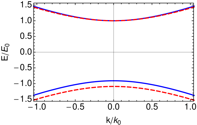
Figure 1: Spin-resolved band dispersions for monolayer MoS₂ at the ${\bm{\mathrm{K}}}$ point. Spin-$\uparrow$($\downarrow$) bands are shown as the blue solid (red dashed) curves. The unit scales for energy $E$ and wave vector ${\bm{\mathrm{k}}}$ (measured from ${\bm{\mathrm{K}}}$) are given in terms of band-structure parameters as $E_{0}\equiv\Delta/2$ and $k_{0}\equiv\Delta/(2at)$. Reversal of all spin labels yields the corresponding band dispersions at the ${\bm{\mathrm{K^{\prime}}}}(\equiv-{\bm{\mathrm{K}}})$ point.

The eigenenergies and eigenstates of the Hamiltonian $H_{0}^{\tau}$ are straightforwardly obtained as

$$E^{(\tau,s)}_{{\bm{\mathrm{k}}}\alpha}=\frac{E_{0}}{2}\left(s\tau\bar{\lambda}+\alpha\sqrt{4\bar{k}^{2}+m_{s\tau}^{2}}\right)$$ (4)

and

$$\psi^{(\tau,s)}_{{\bm{\mathrm{k}}}\alpha}=\frac{1}{\sqrt{2}}\begin{pmatrix}\alpha\left[1+\frac{\alpha m_{s\tau}}{\sqrt{4\bar{k}^{2}+m_{s\tau}^{2}}}\right]^{\frac{1}{2}}\\[8.53581pt] \tau\left[1-\frac{\alpha m_{s\tau}}{\sqrt{4\bar{k}^{2}+m_{s\tau}^{2}}}\right]^{\frac{1}{2}}\mathrm{e}^{-i\tau\theta}\end{pmatrix}\otimes\left|\,s\right\rangle~{},$$ (5)

respectively, where $\alpha=1\,(-1)$ for conduction electrons (valence-band holes), $s=\pm 1$ labels the eigenstates of $s_{z}$, and $m_{\pm}\equiv 2\mp\bar{\lambda}$. We introduced dimensionless quantities $\bar{k}=k/k_{0}$, $\bar{\lambda}\equiv\lambda/E_{0}$, with unit scales for energy and wave vector given by $E_{0}\equiv\Delta/2$ and $k_{0}\equiv\Delta/(2at)$, respectively.  Figure 1 shows the electron and hole band dispersions obtained for MoS₂. Note that SOC gives rise to an energy splitting for the hole (valence-band) excitations that is finite ($\equiv 2\lambda$) even at the band edge. For non-zero wave vector, inter-band coupling induces a spin splitting also for conduction electrons, but its magnitude is suppressed because of the relatively large band gap.

When the Fermi energy $E_{\text{F}}$ is above (below) the conduction-band (valence-band) edge, the system is electron-doped (hole-doped). The Fermi wave vectors for electronic excitations associated with the spin-split bands in each valley are then given by $k^{(s\tau)}_{\text{F}}$, with

$$k^{(\pm)}_{\text{F}}=k_{0}\,\sqrt{\left[(E_{\text{F}}/E_{0})-1\right]\left[(E_{\text{F}}/E_{0})+1\mp\bar{\lambda}\right]}\quad.$$ (6)

The total sheet density $n$ of charge carriers can be related to the Fermi wave vectors via

$$n=\frac{1}{4\pi}\sum_{\tau,s}\left(k_{\text{F}}^{(s\tau)}\right)^{2}\equiv\frac{g_{v}}{4\pi}\left[\left(k_{\text{F}}^{(+)}\right)^{2}+\left(k_{\text{F}}^{(-)}\right)^{2}\right]\,,$$ (7)

where $g_{v}=2$ is the degeneracy factor associated with the valley degree of freedom. In the following, it will be useful to also define a density-related average Fermi wave number $k_{\text{F}}$ such that $n=g_{v}g_{s}k_{\text{F}}^{2}/(4\pi)$, with real-spin degeneracy factor $g_{s}=2$. Obviously we have

$$k_{\text{F}}=\left\{\begin{array}[]{cl}k_{0}\left[\left(\frac{E_{\text{F}}}{E_{0}}\right)^{2}-1\right]^{\frac{1}{2}}&E_{\text{F}}>E_{0}\mbox{ or }E_{\text{F}}<-E_{0}-\lambda\\[8.53581pt] k_{\text{F}}^{(+)}&-E_{0}+\lambda>E_{\text{F}}>-E_{0}-\lambda\end{array}\right..$$ (8)

II.2 Spin susceptibility for a multi-band system

The influence of spin-dependent external stimuli on a many-particle system can be quite generally discussed, within linear-response theory, in terms of the spin susceptibility given byGiuliani and Vignale (2005)

$$\chi_{ij}({\bm{\mathrm{r}}}-{\bm{\mathrm{r}}}^{\prime})=-\frac{i}{\hbar}\int_{0}^{\infty}dt~{}\mathrm{e}^{-\eta t}~{}\langle[S_{i}({\bm{\mathrm{r}}},t),S_{j}({\bm{\mathrm{r}}}^{\prime},0)]\rangle\,.$$ (9)

Here $S_{j}({\bm{\mathrm{r}}})$ denotes a general Cartesian component of the spin-density operator (we measure spin in units of $\frac{\hbar}{2}$), and ${\bm{\mathrm{r}}}$ is the position vector in the $xy$-plane. We can express $S_{j}({\bm{\mathrm{r}}})$ in terms of the second-quantized particle creation and annihilation operators $\Psi^{\dagger}$, $\Psi$ and the spin matrices $\hat{\mathcal{J}}_{j}$ as $S_{j}({\bm{\mathrm{r}}})=\Psi^{\dagger}({\bm{\mathrm{r}}})\hat{\mathcal{J}}_{j}\Psi({\bm{\mathrm{r}}})$. As particle excitations are generally superpositions of contributions from the individual valleys, we represent the particle operator as a spinor, $\Psi({\bm{\mathrm{r}}})=\big{(}\Psi^{(+)}({\bm{\mathrm{r}}}),\Psi^{(-)}({\bm{\mathrm{r}}})\big{)}$. In terms of energy eigenstates and their annihilation operators $c^{(\tau,s)}_{{\bm{\mathrm{k}}}\alpha}$, the contributions for each valley can be expressed as

$$\Psi^{\tau}({\bm{\mathrm{r}}})=\sum_{s,\alpha}\int\frac{d^{2}k}{(2\pi)^{2}}~{}\mathrm{e}^{i({\bm{\mathrm{k}}}+\tau{\bf K}){\bm{\mathrm{r}}}}~{}\psi^{(\tau,s)}_{{\bm{\mathrm{k}}}\alpha}~{}c^{(\tau,s)}_{{\bm{\mathrm{k}}}\alpha}~{}.$$ (10)

With these definitions, the spin susceptibility in Eq. (9) can be written as the Fourier transform of the wave-vector-dependent spin susceptibility $\chi_{ij}({\bf q})$,

$$\chi_{ij}({\bf R})=\int\frac{d^{2}q}{(2\pi)^{2}}~{}\mathrm{e}^{i{\bf q}{\bf R}}~{}\chi_{ij}({\bf q})~{},$$ (11)

where ${\bf R}\equiv{\bm{\mathrm{r}}}-{\bm{\mathrm{r}}}^{\prime}$ and 

$$\chi_{ij}({\bf q}) = \sum_{s,s^{\prime},\tau}\sum_{\alpha,\beta}\int\frac{d^{2}k}{(2\pi)^{2}}~{}\mathscr{W}_{ij({\bm{\mathrm{k}}},{\bm{\mathrm{k}}}+{\bm{\mathrm{q}}},\alpha,\beta)}^{s,s^{\prime},\tau}$$ (12a)

$$\hskip 42.67912pt\times~{}\frac{n_{\text{F}}\big{(}E^{(\tau,s)}_{{\bm{\mathrm{k}}}\alpha}\big{)}-n_{\text{F}}\big{(}E^{(\tau,s^{\prime})}_{{\bm{\mathrm{k}}}+{\bm{\mathrm{q}}}\beta}\big{)}}{E^{(\tau,s)}_{{\bm{\mathrm{k}}}\alpha}-E^{(\tau,s^{\prime})}_{{\bm{\mathrm{k}}}+{\bm{\mathrm{q}}}\beta}+i\eta}~{},\quad$$

with matrix elements

$$\mathscr{W}_{ij({\bm{\mathrm{k}}},{\bm{\mathrm{k}}}^{\prime},\alpha,\beta)}^{(s,s^{\prime},\tau)}=\left[(\psi^{(\tau,s)}_{{\bm{\mathrm{k}}}\alpha})^{\dagger}\hat{J}_{i}\psi^{(\tau,s^{\prime})}_{{\bm{\mathrm{k}}}^{\prime}\beta}\right]\left[(\psi^{(\tau,s^{\prime})}_{{\bm{\mathrm{k}}}^{\prime}\beta})^{\dagger}\hat{J}_{j}\psi^{(\tau,s)}_{{\bm{\mathrm{k}}}\alpha}\right]~{}.$$

See the Appendix for more mathematical details. Here $n_{\text{F}}(\cdot)$ denotes the Fermi function. For our cases of interest, the two valleys make identical contributions to the spin susceptibility, hence we can account for the valley degree of freedom by a degeneracy factor $g_{v}=2$.

It follows from the structure of the spin matrices, Eqs. (2), that the in-plane components $\chi_{xx}({\bm{\mathrm{q}}})=\chi_{yy}({\bm{\mathrm{q}}})$ contain contributions only for $s\neq s^{\prime}$. In contrast, $\chi_{zz}({\bm{\mathrm{q}}})$ has only terms with $s=s^{\prime}$ contributing, thus $\chi_{zz}({\bm{\mathrm{q}}})$ is proportional to the Lindhard function $\chi_{0}({\bm{\mathrm{q}}})$ calculated in Ref. Scholz et al., 2013. By similar arguments, it can be established that all off-diagonal elements of the spin-susceptibility tensor vanish. As the Hamiltonian (3) has axial symmetry, it follows that the spin susceptibility depends only on the magnitude $q\equiv|{\bm{\mathrm{q}}}|$ of the wave vector ${\bm{\mathrm{q}}}$.

III Spin susceptibility of electrons: Extrinsic vs. intrinsic contributions

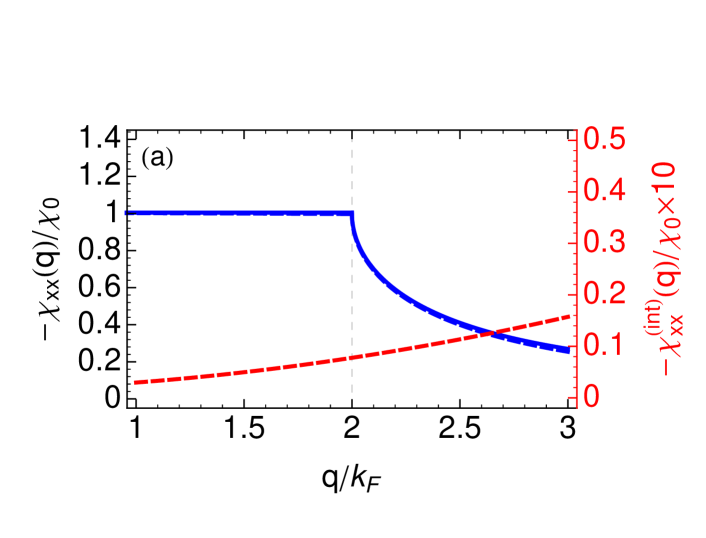
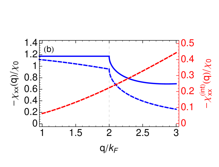
Figure 2: In-plane component $\chi_{xx}(q)\equiv\chi_{xx}^{(\text{ext})}(q)+\chi^{(\text{int})}_{xx}(q)$ of the wave-vector-dependent spin-susceptibility tensor for electron-doped monolayer MoS₂ (blue solid curves). We also plot the extrinsic (intrinsic) contributions $\chi_{xx}^{(\text{ext})}$ $\big{(}\chi^{(\text{int})}_{xx}\big{)}$ separately as the blue (red) dashed curves. Panel (a) [(b)] is for electron density $n=1\times 10^{12}\,$cm^-2 [$5\times 10^{13}\,$cm^-2]. Notice the sharp feature exhibited by $\chi_{xx}$ and $\chi_{xx}^{(\text{ext})}$ for $q\approx 2k_{\text{F}}$ and the different ordinate scale for $\chi^{(\text{int})}_{xx}$.

In this Section, we consider the situation where the Fermi energy is above the conduction-band edge, i.e., $E_{\text{F}}>\Delta/2$. As in the previously considered case of the dielectric polarizability of monolayer graphene Ando (2006); Hwang and Das Sarma (2007); Pyatkovskiy (2009); Scholz and Schliemann (2011); Scholz et al. (2012), the spin-response function of the electron-doped system can be separated into an extrinsic contribution that is entirely due to the occupied states in the conduction band and the intrinsic contribution arising from the completely filled valence band. For the non-vanishing diagonal elements, we find $\chi_{jj}({\bm{\mathrm{q}}})=\chi_{jj}^{(\text{ext})}({\bm{\mathrm{q}}})+\chi_{jj}^{(\text{int})}({\bm{\mathrm{q}}})$, with

$$\chi_{jj}^{(\text{ext})}({\bm{\mathrm{q}}}) = \sum_{s,s^{\prime},\tau\atop\delta=\pm 1}\int\frac{d^{2}k}{(2\pi)^{2}}~{}~{}n_{\text{F}}\big{(}E^{(\tau,s)}_{{\bm{\mathrm{k}}}+}\big{)}$$

$$\times\left[\frac{\mathscr{W}_{jj({\bm{\mathrm{k}}},{\bm{\mathrm{k}}}+{\bm{\mathrm{q}}},+,+)}^{(s,s^{\prime},\tau)}}{E^{(\tau,s)}_{{\bm{\mathrm{k}}}+}-E^{(\tau,s^{\prime})}_{{\bm{\mathrm{k}}}+{\bm{\mathrm{q}}}+}+i\eta\delta}+\frac{\mathscr{W}_{jj({\bm{\mathrm{k}}},{\bm{\mathrm{k}}}+{\bm{\mathrm{q}}},+,-)}^{(s,s^{\prime},\tau)}}{E^{(\tau,s)}_{{\bm{\mathrm{k}}}+}-E^{(\tau,s^{\prime})}_{{\bm{\mathrm{k}}}+{\bm{\mathrm{q}}}-}+i\eta\delta}\right]\,,$$

$$\chi_{jj}^{(\text{int})}({\bm{\mathrm{q}}}) = -\sum_{s,s^{\prime},\tau\atop\delta=\pm 1}\int\frac{d^{2}k}{(2\pi)^{2}}~{}~{}\frac{\mathscr{W}_{jj({\bm{\mathrm{k}}},{\bm{\mathrm{k}}}+{\bm{\mathrm{q}}},+,-)}^{(s,s^{\prime},\tau)}~{}n_{\text{F}}\big{(}E^{(\tau,s)}_{{\bm{\mathrm{k}}}-}\big{)}}{E^{(\tau,s)}_{{\bm{\mathrm{k}}}+}-E^{(\tau,s^{\prime})}_{{\bm{\mathrm{k}}}+{\bm{\mathrm{q}}}-}+i\eta\delta}~{}.$$

The expressions in Eqs. (13) have been obtained from Eq. (12a) using the axial symmetry of the Hamiltonian (3). In the zero-temperature limit (which we employ in the following), the Fermi functions are $n_{\text{F}}\big{(}E^{(\tau,s)}_{{\bm{\mathrm{k}}}+}\big{)}=\Theta\big{(}k^{(s\tau)}_{\text{F}}-k\big{)}$ and $n_{\text{F}}\big{(}E^{(\tau,s)}_{{\bm{\mathrm{k}}}-}\big{)}=1$, respectively.

III.1 In-plane spin-susceptibility component $\mathbf{\chi_{xx}}$

An explicit calculation of the extrinsic contribution to the in-plane spin susceptibility tensor element yields

$$\chi^{\text{(ext)}}_{xx}(q) = -\frac{\chi_{0}}{4}\Biggl{\{}\frac{2\bar{q}^{4}+{\mathcal{F}}\bar{\lambda}^{2}(6+\bar{\lambda}+{\mathcal{G}})-\bar{q}^{2}[{\mathcal{G}}~{}{\mathcal{F}}+\bar{\lambda}({\mathcal{F}}+8\bar{\lambda})]}{(\bar{q}^{2}-\bar{\lambda}^{2})^{2}}+2\left(\sqrt{4\big{(}{\bar{k}^{(+)}_{\text{F}}}\big{)}^{2}+m_{+}^{2}}-m_{+}\right)\Biggr{.}$$ (14)

$$\hskip 42.67912pt\Biggl{.}+\frac{\left[\bar{q}^{6}-2\bar{q}^{2}\bar{\lambda}^{2}+2\bar{\lambda}^{4}(\bar{\lambda}^{2}-4)-\bar{q}^{4}(\bar{\lambda}^{2}+4)\right]}{(\bar{\lambda}^{2}-\bar{q}^{2})^{5/2}}\ln{\frac{\bar{q}^{2}\left(\sqrt{\bar{\lambda}^{2}-\bar{q}^{2}}-2\right)}{{\mathcal{F}}\sqrt{\bar{\lambda}^{2}-\bar{q}^{2}}+\bar{\lambda}^{2}({\mathcal{G}}-m_{+})-\bar{q}^{2}({\mathcal{G}}+\bar{\lambda})}}\Biggr{\}}~{},\quad$$

with $\chi_{0}=g_{v}g_{s}k_{0}^{2}/(2\pi E_{0})\equiv\Delta/(\pi a^{2}t^{2})$. We have also used the abbreviations

$${\mathcal{F}}=\sqrt{\bar{q}^{4}-2\bar{q}^{2}\bar{\lambda}({\mathcal{G}}-m_{+})-2\bar{\lambda}^{2}m_{+}({\mathcal{G}}-m_{+})+4\kappa_{q}^{2}(\bar{\lambda}^{2}-\bar{q}^{2})}\,\,,$$ (15)

$${\mathcal{G}} = \sqrt{4\kappa_{q}^{2}+m_{+}^{2}}\quad,$$ (16)

$$\kappa_{q} = \mathcal{K}_{q}\,\Theta\left(k_{\text{F}}^{(+)}+k_{\text{F}}^{(-)}-q\right)+\bar{k}_{\text{F}}^{(+)}\,\Theta\left(q-k_{\text{F}}^{(+)}-k_{\text{F}}^{(-)}\right),$$

$$\mathcal{K}_{q} = \frac{\bar{q}^{3}-\bar{q}\bar{\lambda}(\bar{\lambda}-2)-\bar{q}\bar{\lambda}\sqrt{4+\bar{q}^{2}-\bar{\lambda}^{2}}}{2(\bar{q}^{2}-\bar{\lambda}^{2})}\quad.$$ (18)

In the limit $q\to 0$, the result

$$\chi^{\text{(ext)}}_{xx}(0) = -\frac{\chi_{0}}{2}\Biggl{(}\frac{(4-\bar{\lambda}^{2})~{}\text{arctanh}\frac{\bar{\lambda}}{2}}{\bar{\lambda}}\Biggr{.}$$ (19)

$$\hskip 42.67912pt\Biggl{.}+\sqrt{4\big{(}{\bar{k}^{(+)}_{\text{F}}}\big{)}^{2}+m_{+}^{2}}-m_{+}\Biggl{)}\quad$$

is found.

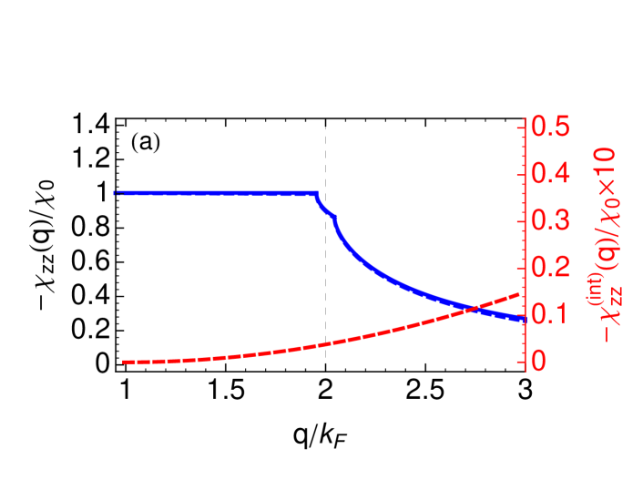
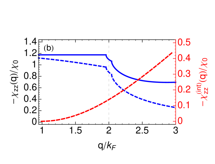
Figure 3: Spin-susceptibility component $\chi_{zz}(q)\equiv\chi_{zz}^{(\text{ext})}(q)+\chi^{(\text{int})}_{zz}(q)$ for electron-doped monolayer MoS₂ (blue solid curves). The extrinsic (intrinsic) contributions $\chi_{zz}^{(\text{ext})}$ $\big{(}\chi^{(\text{int})}_{zz}\big{)}$ are also plotted as the blue (red) dashed curves. Panel (a) [(b)] shows results for electron density $n=1\times 10^{12}\,$cm^-2 [$5\times 10^{13}\,$cm^-2]. Sharp features are exhibited by $\chi_{zz}$ and $\chi_{zz}^{(\text{ext})}$ for $q=k_{\text{F}}^{(+)},k_{\text{F}}^{(-)}$. Note the different scale for $\chi^{(\text{int})}_{zz}$.

The intrinsic contribution can be expressed as

$$\chi^{\text{(int)}}_{xx}(q) = -\left.\chi^{\text{(ext)}}_{xx}(q)\right|_{\kappa_{q}\equiv\mathcal{K}_{q}}+\chi^{\text{(ext)}}_{xx}(0)+\chi^{\text{(int)}}_{xx}(0)\,\,,$$

with $\chi^{\text{(ext)}}_{xx}(0)$ from Eq. (19). In contrast to the static dielectric polarizability of both monolayer MoS₂Scholz et al. (2013) and monolayer graphene Ando (2006); Hwang and Das Sarma (2007); Pyatkovskiy (2009); Scholz and Schliemann (2011); Scholz et al. (2012), the in-plane spin susceptibility of electron-doped transition metal dichalcogenides is found to have a finite intrinsic contribution for $q\to 0$,

$$\chi^{\text{(int)}}_{xx}(0)=-\frac{\chi_{0}}{2}\left(\frac{2\bar{\lambda}-(4-\bar{\lambda}^{2})~{}\text{arctanh}\frac{\bar{\lambda}}{2}}{\bar{\lambda}}\right)\quad.$$ (21)

As the expression (21) vanishes for $\lambda\to 0$, the finite $\chi^{\text{(int)}}_{xx}(0)$ is a SOC effect. Combining Eqs. (21) and (19) yields the $q\to 0$ limit of the in-plane spin-susceptibility tensor component in the electron-doped case given by

$$\chi_{xx}(0) = -\frac{\chi_{0}}{2}\left(\sqrt{4\big{(}\bar{k}^{(+)}_{\text{F}}\big{)}^{2}+m_{+}^{2}}+\bar{\lambda}\right)\,,$$ (22a)

$$\equiv -\chi_{0}\,\frac{E_{\text{F}}}{E_{0}}\quad.$$ (22b)

Figure 2 illustrates the behavior of $\chi_{xx}(q)$ and also shows the individual extrinsic and intrinsic contributions. A cancellation of the latters’ $q$ dependences yield a constant $\chi_{xx}(q)$ for $q\leq k^{(+)}_{\text{F}}+k^{(-)}_{\text{F}}$ ($\approx 2k_{\text{F}}$ typically), which is followed by an abrupt decrease of the spin susceptibility for $q>k^{(+)}_{\text{F}}+k^{(-)}_{\text{F}}$. The general line shape is similar to the one found for an ordinary 2D electron gas Giuliani and Vignale (2005) in the absence of spin-orbit coupling, and the plateau behavior is also exhibited by response functions of monolayer graphene Ando (2006); Hwang and Das Sarma (2007); Pyatkovskiy (2009); Scholz and Schliemann (2011). The fact that only a single sharp feature appears in $\chi_{xx}(q)$, even though there are two Fermi surfaces for the values of density used for the plots, originates from the in-plane response being governed by transitions between eigenstates with opposite $s_{z}$ quantum number. Furthermore, in contrast to the case of an ordinary 2D electron gas, the plateau value of $\chi_{xx}(q)$ is density dependent [see Eq. (22)], but this dependence is much weaker than in the case of grapheneAndo (2006); Hwang and Das Sarma (2007); Pyatkovskiy (2009); Scholz and Schliemann (2011) because of the relatively large value of the gap parameter $\Delta$.

III.2 Perpendicular spin-susceptibility component $\mathbf{\chi_{zz}}$

The extrinsic contribution to the spin-susceptibility component describing the response in the direction perpendicular to the 2D material’s plane is the sum of terms arising from the individual spin-split bands,

$$\chi^{\text{(ext)}}_{zz}(q)=\sum_{s}\chi^{\text{(ext)}}_{zz,s}(q)\quad,$$ (23a)

$$\chi^{\text{(ext)}}_{zz,s}(q) = \frac{\chi_{0}}{8}\left\{m_{s}-2\sqrt{4\big{(}\bar{k}^{(s)}_{\text{F}}\big{)}^{2}+m_{s}^{2}}-\frac{(m_{s}^{2}-\bar{q}^{2})}{\bar{q}}\arctan\frac{\bar{q}}{m_{s}}\right\}\Theta\big{(}2k^{(s)}_{\text{F}}-q\big{)}$$ (23b)

$$+\,\frac{\chi_{0}}{8}\left\{m_{s}-2\sqrt{\big{(}\bar{k}^{(s)}_{\text{F}}\big{)}^{2}+m_{s}^{2}}+\frac{1}{\bar{q}}\sqrt{\left[4\big{(}\bar{k}^{(s)}_{\text{F}}\big{)}^{2}+m_{s}^{2}\right]\left[\bar{q}^{2}-4\big{(}\bar{k}^{(s)}_{\text{F}}\big{)}^{2}\right]}-\frac{m_{s}^{2}-\bar{q}^{2}}{\bar{q}}\Biggl{[}2\arcsin\sqrt{\frac{4\big{(}\bar{k}^{(s)}_{\text{F}})^{2}+m_{s}^{2}}{m_{s}^{2}+\bar{q}^{2}}}\right.$$

$$\left.-\,2\arctan\frac{m_{s}}{\bar{q}}+\frac{1}{2}\arctan\left(\frac{m_{s}}{2\bar{q}}-\frac{\bar{q}}{2m_{s}}\right)-\frac{1}{2}\arctan\frac{8\big{(}\bar{k}^{(s)}_{\text{F}}\big{)}^{2}+m_{s}^{2}-\bar{q}^{2}}{2\sqrt{4\big{(}\bar{k}^{(s)}_{\text{F}}\big{)}^{2}+m_{s}^{2}}\sqrt{\bar{q}^{2}-4\big{(}\bar{k}^{(s)}_{\text{F}}\big{)}^{2}}}\Biggr{]}\right\}\Theta\big{(}q-2k^{(s)}_{\text{F}}\big{)}\,.\quad$$

In the $q\to 0$ limit, Eq. (23a) yields

$$\chi^{\text{(ext)}}_{zz}(0)=-\frac{\chi_{0}}{4}\sum_{s}\sqrt{4\big{(}\bar{k}^{(s)}_{\text{F}})^{2}+m_{s}^{2}}~{},$$ (24)

thus $-\chi^{\text{(ext)}}_{zz}(0)$ corresponds to the density of states at the Fermi energy. For the intrinsic contribution, the expression

$$\chi^{\text{(int)}}_{zz}(q)=-\frac{\chi_{0}}{8}\sum_{s}\left[m_{s}-\frac{m_{s}^{2}-\bar{q}^{2}}{\bar{q}}\arctan\frac{\bar{q}}{m_{s}}\right]$$ (25)

is found, which vanishes in the limit $q\to 0$. As a result, $\chi_{zz}(0)\equiv\chi^{\text{(ext)}}_{zz}(0)$, and we find using Eq. (24)

$$\chi_{zz}(0)=-\chi_{0}\,\frac{E_{\text{F}}}{E_{0}}\equiv\chi_{xx}(0)\quad.$$ (26)

The line shape of $\chi_{zz}(q)$ is shown in Fig. 3 for band-structure parameters of MoS₂ and two density values. As in the case of the in-plane spin-susceptibility component, a cancellation of $q$ dependences from the extrinsic and intrinsic contributions results in a plateau for $\chi_{zz}(q)$ for wave vectors smaller than a threshold value (here: $2k^{(+)}_{\text{F}}$). While the plateau value is the same as for $\chi_{xx}(q)$, its width is different. Also in contrast to the behavior of $\chi_{xx}(q)$, two sharp features at $q=k^{(+)}_{\text{F}}$ and at $q=k^{(-)}_{\text{F}}$ signify the existence of the two Fermi surfaces. However, the line shapes of the in-plane and perpendicular spin-susceptibility components become very similar again for $q>2k^{(-)}_{\text{F}}$. Hence, except for wave vectors within the region close to the two Fermi wave vectors, the spin response of charge carriers in electron-doped transition metal dichalcogenides is isotropic and very similar to that of an ordinary 2D electron gas Giuliani and Vignale (2005). Differences to the standard behavior will therefore occur in the oscillations of the spin susceptibility in real space [Eq. (11)] whose wave length and beating pattern is governed by the sharp features in $\chi_{ij}(q)$.

IV Spin susceptibility of holes: In-plane/out-of-plane anisotropy

Specializing the general definition (12a) for the spin-susceptibility tensor to the situation where only states in the valence band are occupied [i.e., for $n_{\text{F}}\big{(}E^{(\tau,s)}_{{\bm{\mathrm{k}}}+}\big{)}\equiv 0$], we obtain

$$\chi_{jj}({\bm{\mathrm{q}}})=\sum_{s,s^{\prime},\tau\atop\delta=\pm 1}\int\frac{d^{2}k}{(2\pi)^{2}}~{}n_{\text{F}}\big{(}E^{(\tau,s)}_{{\bm{\mathrm{k}}}-}\big{)}$$

$$\times\left[\frac{\mathscr{W}_{jj({\bm{\mathrm{k}}},{\bm{\mathrm{k}}}+{\bm{\mathrm{q}}},-,-)}^{(s,s^{\prime},\tau)}}{E^{(\tau,s)}_{{\bm{\mathrm{k}}}-}-E^{(\tau,s^{\prime})}_{{\bm{\mathrm{k}}}+{\bm{\mathrm{q}}}-}+i\eta\delta}+\frac{\mathscr{W}_{jj({\bm{\mathrm{k}}},{\bm{\mathrm{k}}}+{\bm{\mathrm{q}}},-,+)}^{(s,s^{\prime},\tau)}}{E^{(\tau,s)}_{{\bm{\mathrm{k}}}-}-E^{(\tau,s^{\prime})}_{{\bm{\mathrm{k}}}+{\bm{\mathrm{q}}}+}+i\eta\delta}\right].\quad$$ (27)

Note the analogy of the expression (IV) with that of the extrinsic part of the electron-doped case [cf. Eq. (13)]. 

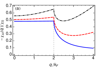
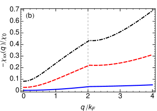
Figure 4: Spin response of hole-doped monolayer MoS₂. Panel (a) [(b)] shows $\chi_{zz}(q)$ [$\chi_{xx}(q)$] obtained for a hole sheet density $n=1\times 10^{12}$cm^-2 (blue solid curve), $n=1\times 10^{13}$cm^-2 (red dashed curve), and $n=3\times 10^{13}$cm^-2 (black dot-dashed curve). Noteworthy features are the strong in-plane/out-of-plane anisotropy of the spin response, the deviations from ideal 2D-electron-gas behavior even for $\chi_{zz}(q)$, which are getting more pronounced as the density increases, and the nonanalyticity exhibited by $\chi_{zz}(q)$ [$\chi_{xx}(q)$] for $q=2k_{\text{F}}\equiv 2k_{\text{F}}^{(+)}$ [$q=k_{1}>2k_{\text{F}}^{(+)}$].

In the following, we consider the situation where hole densities $n$ are small enough so that only the upper-most of the two spin-split valence bands has empty states. This implies $\Delta/2-\lambda<-E_{\text{F}}<\Delta/2+\lambda$, and there will be only one Fermi surface with radius $k_{\text{F}}^{(+)}\equiv\sqrt{4\pi n/g_{v}}$. For this situation, we obtain in the zero-temperature limit the in-plane component of the spin-susceptibility tensor as $\chi_{xx}({\bm{\mathrm{q}}})=\chi^{(1)}_{xx}({\bm{\mathrm{q}}})+\chi^{(2)}_{xx}({\bm{\mathrm{q}}})$, where

$$\chi^{(1)}_{xx}(q)=$$

$$-\frac{\chi_{0}}{8}\Biggl{\{}\frac{2\bar{q}^{4}(1-\bar{\lambda})+\bar{\lambda}^{2}\left[{\mathcal{H}}(\tilde{\mathcal{G}}-6-\bar{\lambda})+4\bar{\lambda}(4-\bar{\lambda}^{2})\right]+\bar{q}^{2}[\bar{\lambda}(8+{\mathcal{H}}-8\bar{\lambda}+6\bar{\lambda}^{2})-\tilde{\mathcal{G}}\,{\mathcal{H}}]}{(\bar{q}^{2}-\bar{\lambda}^{2})^{2}}+2\left(\sqrt{4\big{(}{\bar{k}^{(+)}_{\text{F}}}\big{)}^{2}+m_{+}^{2}}-m_{+}\right)\Biggr{.}$$

$$\hskip 42.67912pt\Biggl{.}+\,\frac{\left[\bar{q}^{6}-2\bar{q}^{2}\bar{\lambda}^{2}+2\bar{\lambda}^{4}(\bar{\lambda}^{2}-4)-\bar{q}^{4}(\bar{\lambda}^{2}+4)\right]}{(\bar{\lambda}^{2}-\bar{q}^{2})^{5/2}}~{}\ln{\frac{\bar{q}^{2}\left(2\bar{\lambda}-2+\sqrt{\bar{\lambda}^{2}-\bar{q}^{2}}\right)+2\bar{\lambda}m_{+}\left(\sqrt{\bar{\lambda}^{2}-\bar{q}^{2}}+\bar{\lambda}\right)}{{\mathcal{H}}\sqrt{\bar{\lambda}^{2}-\bar{q}^{2}}+\bar{\lambda}^{2}(m_{+}+\tilde{\mathcal{G}})+\bar{q}^{2}(\bar{\lambda}-\tilde{\mathcal{G}})}}\Biggr{\}}~{},$$ (28)

and $\chi^{(2)}_{xx}({\bm{\mathrm{q}}})=\chi^{(\text{int})}_{xx}({\bm{\mathrm{q}}})$ given in Eq. (III.1). We have again introduced abbreviations

$${\mathcal{H}}=\sqrt{\bar{q}^{4}+2\bar{q}^{2}\bar{\lambda}(\tilde{\mathcal{G}}+m_{+})+2\bar{\lambda}^{2}m_{+}(\tilde{\mathcal{G}}+m_{+})+4\tilde{\kappa}_{q}^{2}(\bar{\lambda}^{2}-\bar{q}^{2})}\quad,$$ (29)

$$\tilde{\mathcal{G}} = \sqrt{4\tilde{\kappa}_{q}^{2}+m_{+}^{2}}\quad,$$ (30)

$$\tilde{\kappa}_{q} = \mathcal{K}_{q}\,\Theta\left(k_{1}-q\right)+\bar{k}_{\text{F}}^{(+)}\,\Theta\left(q-k_{1}\right),$$ (31)

$$\frac{k_{1}}{k_{0}} = \bar{k}_{\text{F}}^{(+)}+\left[\big{(}\bar{k}_{\text{F}}^{(+)}\big{)}^{2}+\bar{\lambda}\left(\sqrt{4\big{(}\bar{k}_{\text{F}}^{(+)}\big{)}^{2}+m_{+}^{2}}-m_{+}\right)\right]^{\frac{1}{2}},$$

with ${\mathcal{K}}_{q}$ from Eq. (18). Note that $\chi_{xx}(q)$ is nonanalytic at $q=k_{1}\,\big{(}>2k^{(+)}_{\text{F}}\big{)}$. In the limit $q\to 0$, Eq. (IV) yields

$$\chi_{xx}^{(1)}(0)=-\frac{\chi_{0}}{4}\left(\sqrt{4\big{(}{\bar{k}^{(+)}_{\text{F}}}\big{)}^{2}+m_{+}^{2}}-m_{+}\right)~{}.$$ (33)

The general result for the spin-susceptibility tensor component perpendicular to the plane is obtained as

$$\chi_{zz}(q)=\sum_{s}\left(\chi_{zz,s}^{(1)}(q)~{}\Theta\big{(}k_{\text{F}}^{(s)}\big{)}+\chi_{zz,s}^{(2)}(q)\right)~{},$$ (34)

where $\chi_{zz,s}^{(1)}(q)=\chi_{zz,s}^{(\text{ext})}(q)$ and $\chi_{zz,s}^{(2)}(q)=\chi_{zz,s}^{(\text{int})}(q)$, with the expressions for $\chi_{zz,s}^{(\text{ext})}(q)$ and $\chi_{zz,s}^{(\text{int})}(q)$ from Eqs. (23b) and (25), respectively. Unlike in the electron-doped case, SOC does not give rise to the existence of two Fermi surfaces for all hole densities. For our case of interest where hole densities are low enough such that only the upper-most valence band has empty states, only a single Fermi surface exists. In this situation, the $q\to 0$ limit yields

$$\chi_{zz}(0)=-\frac{\chi_{0}}{4}\,\sqrt{4\big{(}\bar{k}^{(+)}_{\text{F}}\big{)}^{2}+m_{+}^{2}}\equiv\frac{\chi_{0}}{2}\,\left(\frac{E_{\text{F}}}{E_{0}}-\frac{\bar{\lambda}}{2}\right)~{},$$

which corresponds to the density of states in the upper-most valence band. In contrast to the in-plane spin-susceptibility component, $\chi_{zz}(q)$ is non-analytic at $q=2k^{(+)}_{\text{F}}$. Also, $|\chi_{zz}(0)|\gg|\chi_{xx}(0)|$ for typical hole densities, signifying a strong anisotropy of the spin response.

The behavior of the spin response in the hole-doped case differs markedly from the electron-doped situation. See Fig. 4 for an illustration. As a first observation, a strong dependence on hole-sheet density is apparent. In the low-density regime, the in-plane spin response is almost uniformly very small, whereas $\chi_{zz}(q)$ has the line shape associated with the response functions of an ordinary 2D electron system Giuliani and Vignale (2005). As the hole density increases, a pronounced peak develops in $\chi_{xx}(q)$ for $q=k_{1}\gtrsim 2k_{\text{F}}^{(+)}$, and the plateau behavior of $\chi_{zz}(q)$ disappears. Some of these features are very similar to those exhibited by the spin response of 2D hole systems Kernreiter et al. (2013) realized by a quantum-well confinement in typical semiconductor heterostructures Winkler (2003). The nonanalyticity at (near) $q=2k_{\text{F}}$ in $\chi_{zz}$ ($\chi_{xx}$) as well as the power-law behavior in its vicinity She and Bishop (2013) determine the decay of the corresponding spin-susceptibility oscillations in real space. This and other consequences of the unusual spin-response properties in the hole-doped case will be discussed in greater detail in the following Section.

V Physical consequences of unusual spin response in the hole-doped case

Based on the results presented in the previous Section, we consider spin-related physical quantities for hole-doped monolayers of transition metal dichalcogenides. We start by discussing the properties of hole-carrier-mediated exchange interaction between localized impurity spins. Then the paramagnetic response of our system of interest is investigated. These examples serve to illustrate the very different behavior of hole-doped systems, in contrast to the electron-doped case that mirrors the properties of ordinary 2D electron gases.

V.1 RKKY interaction and mean-field magnetism

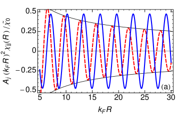
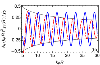
Figure 5: Spin response functions in real space. To highlight deviations from the ordinary 2D-electron-gas behavior Giuliani and Vignale (2005), we plot the quantities $A_{j}\big{(}k_{\text{F}}R\big{)}^{2}\chi_{jj}(R)$ in Panel (a) [(b)] obtained for a hole density $n=1\times 10^{12}$cm^-2 [$n=3\times 10^{13}$cm^-2]. The red dashed (blue solid) curve shows $\chi_{xx}$ ($\chi_{zz}$). The decrease of the oscillation amplitude for $\big{(}k_{\text{F}}R\big{)}^{2}\chi_{xx}(R)$ shows that the in-plane spin response decays faster than the $R^{-2}$ power law expected for ordinary 2D electron systems. The scale factors are $A_{x}=50$ [$5$] and $A_{z}=1$ [$1$] in Panel (a) [(b)], and $\tilde{\chi}_{0}=\chi_{0}k_{\text{F}}^{2}/(2\pi)\equiv 2nk_{0}^{2}/(\pi E_{0})$.

We consider two localized impurity spins ${\bm{\mathrm{I}}}^{(1)}$ and ${\bm{\mathrm{I}}}^{(2)}$ that couple via a contact interaction of strength $J$ to the local spin density of holes in a monolayer transition metal dichalcogenide sample. In second-order perturbation theory, such a coupling gives rise to an effective exchange interaction between the impurity-spin components that is described by the RKKY Hamiltonian Ruderman and Kittel (1954); Kasuya (1956); Yosida (1957)

$$H_{\text{RKKY}}^{(1,2)}=-J^{2}\sum_{i,j}~{}I^{(1)}_{i}\,I^{(2)}_{j}~{}\chi_{ij}({\bm{\mathrm{R}}})~{}.$$ (36)

Here ${\mathbf{R}}$ is the distance vector between the locations of the two impurity spins, and $\chi_{ij}({\bm{\mathrm{R}}})$ denotes the spin susceptibility in real space given by Eq. (11). For our cases of interest, the spin susceptibility turns out to be isotropic in its dependence on real-space position; $\chi_{ij}({\bm{\mathrm{R}}})\equiv\chi_{ij}(R)$.

Figure 5 shows plots of the quantity $\big{(}k_{\text{F}}R\big{)}^{2}\chi_{jj}(R)$ for two realistic values of the hole density. The fact that $\chi_{zz}(R)\propto R^{-2}$ is clearly indicated by the constancy of the oscillations exhibited by the blue solid curves. In contrast, the in-plane response function is seen to decay faster with distance $R$. Closer inspection reveals that $\chi_{zz}(R)\propto R^{-5/2}$, i.e., shows behavior that deviates from the expected $R^{-2}$ power law of a 2D Fermi liquid.  Thus the in-plane RKKY range function for monolayer transition metal dichalcogenides shows behavior that is intermediate between that of an ordinary 2D electron gas Giuliani and Vignale (2005) (or doped graphene Brey et al. (2007)) and undoped graphene Wunsch et al. (2006).

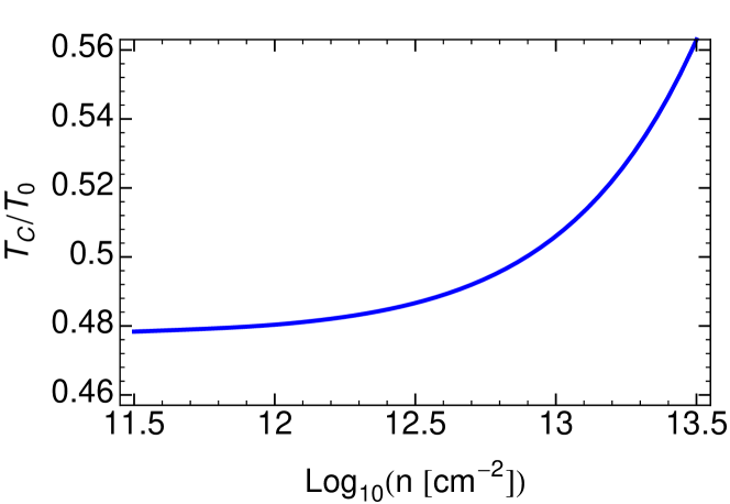
Figure 6: Density dependence of the Curie temperature for hole-mediated easy-axis Ising ferromagnetism of impurity spins in monolayer MoS₂.

In the low-density regime, the amplitude of $\chi_{zz}(R)$ can be more than an order of magnitude larger than that of $\chi_{xx}(R)$; see Fig. 5(a). However, as the density is increased, $\chi_{xx}(R)$ becomes appreciable and even reaches the same magnitude as $\chi_{zz}(R)$; see Fig. 5(b). From the figure, it is also apparent that the oscillations of $\chi_{xx}(R)$ and $\chi_{zz}(R)$ have a relative phase shift that varies somewhat with $R$ and sometimes turns out to be close to $\pi/2$. It follows from this observation that the lowest-energy state of two RKKY-coupled impurity spins can change from the typically expected easy-axis configuration (both impurity spins align in the direction perpendicular to the monolayer plane) to an easy-plane alignment if the distance $R$ corresponds to a point where $\chi_{xx}(R)$ [$\chi_{zz}(R)$] has a maximum [a zero].

Considering now a large number of impurity spins distributed, on average, homogeneously with density $n_{I}$ in the material, the RKKY spin Hamiltonian can be treated using standard mean-field theory Yosida (1996). For the hole-doped situation, we have $|\chi_{zz}(q)|_{q=0}\gg|\chi_{xx}(q)|_{q=0}$, hence the spin system will exhibit Ising-type ferromagnetism with Curie temperature given by

$$T_{\text{C}}=T_{0}~{}\left.\frac{|\chi_{zz}(q)|}{\chi_{0}}\right|_{q=0}~{},$$ (37a)

with the temperature scale

$$T_{0}=\frac{I(I+1)}{3}\,\frac{J^{2}}{k_{\text{B}}}\,n_{I}\,\frac{\Delta}{\pi a^{2}t^{2}}~{}.$$ (37b)

Here $I$ and $n_{I}$ denote the impurity spin quantum number and areal density of impurities, respectively. Due to the density dependence of $\chi_{zz}(q=0)$ [see Eq. (IV)], the Curie temperature can, in principle, be manipulated by the magnitude of hole doping. However, as illustrated in Fig. 6, the range of realistic values for the hole density allows for an adjustment of $T_{\text{C}}$ by only upto 10% in the high-density regime.

In general, mean-field predictions for transition temperatures are only a crude approximation to reality, as the excitation of spin waves generally suppresses – in some cases, even destroys – magnetic order.Simon et al. (2008)

V.2 Pauli paramagnetism and effective $g$-factor

An external magnetic field generally couples to the hole carriers’ spin via a Zeeman term $H_{\text{Z}}=\kappa\,\mu_{\text{B}}\,B_{j}\hat{J}_{j}$, where $\mu_{\text{B}}$ is the Bohr magneton and $2\kappa$ the bulk valence-band $g$ factor.  In the limit of a small magnetic field, the paramagnetic susceptibility is given by

$$\chi_{\text{P},j}=(\kappa\,\mu_{\text{B}})^{2}~{}\chi^{(1)}_{jj}(q)|_{q=0}~{},$$ (38)

where $\chi^{(1)}_{jj}(q)$ are the spin susceptibilities of the hole-doped system for the in-plane and out-of-plane response whose $q\to 0$ limits are shown in Eqs. (33) and (IV). It is possible to define a collective $g$-factor for the charge carriers by expressing the paramagnetic susceptibility in terms of the density of states, which is the zero-$q$ limit of the Lindhard function Giuliani and Vignale (2005) $\chi_{\text{L}}(q)$, as $\chi_{\text{P},j}=(g_{j}\mu_{\text{B}})^{2}\,\chi_{\text{L}}(0)/4$, and equate this with the expression in Eq. (38) to yield Kernreiter et al. (2013)

$$g_{j}=2\kappa\,\sqrt{\left.\frac{\chi^{(1)}_{jj}(q)}{\chi_{\text{L}}(q)}\right|_{q=0}}\quad.$$ (39)

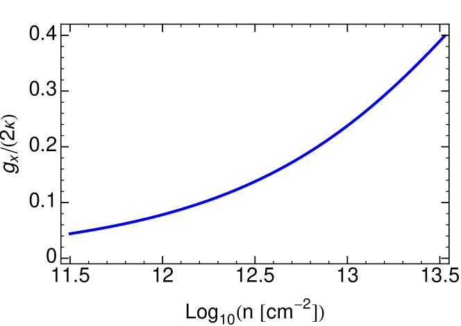
Figure 7: Density dependence of the effective in-plane $g$-factor for hole-doped MoS₂.

Our result for the out-of-plane spin response of holes in monolayer transition metal dichalcogenides implies $g_{z}\equiv 2\kappa$, as $\chi_{zz}(q=0)$ turns out to be equal to the density of states at the Fermi energy. However, the in-plane $g$-factor shows unusual behavior, which is illustrated in Fig. 7. For small densities (small $k_{\text{F}}$), $g_{x}$ is negligible [see Eq. (33)]. In contrast, for large hole densities, $g_{x}$ can become of the same order of magnitude as $g_{z}$.

VI Summary and Conclusions

We have calculated, and obtained analytical expressions for, the wave-vector-dependent static spin susceptibility of charge carriers in monolayer transition metal dichalocogenides. Our approach is based on the effective-mass model description of electronic excitations in these materials. Very different behavior emerges for the cases of electron-doped and hole-doped systems. We illustrate our findings using band parameters of MoS₂ monolayers.

Features exhibited for electron doping are similar, but not entirely analogous, to those associated with ordinary 2D electron gases. The finite SOC results in deviations from the canonical line shape near $q=2k_{\text{F}}$. Also, unlike the ordinary 2D electron system, the plateau value of the spin response at small $q$ depends on the electron sheet density. See Eq. (26). The total response of the electron-doped system is obtained as the sum of an extrinsic part that vanishes without the doping and an intrinsic contribution due to the completely filled valence band.

The hole-doped system shows marked deviations from the behavior expected from an ordinary 2D electron gas. In that, it mirrors some of the features of confined valence-band states in semiconductor heterostructures Dietl et al. (1997); Kernreiter et al. (2013). In particular, a strong anisotropy of the spin susceptibility is exhibited, with the out-of-plane response being much stronger than the in-plane response in the low-density limit. However, the in-plane response is enhanced as the hole density increases and shows pronounced nonanalytic behavior near $q=2k_{\text{F}}$. We have investigated implications for spin-related physical quantities arising from the unusual spin response of the hole-doped system. We show that the oscillations of the in-plane spin response in real space decay faster than the typical $R^{-2}$ law that is expected for a 2D Fermi liquid. Both the Curie temperature for hole-mediated easy-axis ferromagnetism and the $g$ factor characterizing the Zeeman spin splitting due to an in-plane magnetic field are found to be tunable by changing the hole density.

In this work, we have neglected effects due to disorder and electron-electron interactions, which are known to, in principle, alter the spin response of ordinary 2D electron systems Palo et al. (2009). Parameterization in terms of local field factors Giuliani and Vignale (2005); Palo et al. (2009) could be used to shed further light on how interactions renormalize the spin susceptibility of monolayer transition metal dichalcogenides. As far as disorder is concerned, it can be expected that important corrections to our results obtained in the clean limit will only arise for low-enough carrier densities when the difference between $E_{\text{F}}$ and the band edge is comparable in magnitude to the disorder-induced lifetime broadening Cappelluti et al. (2002); De Palo et al. (2005). The latter turns out to be of the order of $\sim\,$0.01 eV in typical samples Radisavljevic et al. (2011) and, therefore, is at least an order of magnitude smaller than all other relevant energy scales.

Our work adds to the understanding of monolayer transition metal dichalcogenides as a new materials system whose charge carriers show behavior that is sometimes reminiscent of – but generally distinct from – other 2D systems. The very different properties exhibited by the electron-doped and hole-doped cases create the possibility for a versatile engineering of electronic systems with specially tailored spin response. To verify our theoretical results, electronic-transport experiments could be used to measure the carrier spin susceptibility in the $q\to 0$ limit Zhu et al. (2003); Vakili et al. (2004). Furthermore, monolayer transition metal dichalcogenides would lend themselves as ideal samples for implementing a recent proposal Stano et al. (2013) for determining the full spatial structure of the spin susceptibility.

*

Appendix A Lehmann-type representation for the static spin susceptibility

Here we give a short derivation of the expression for the wave-vector-dependent spin susceptibility used in our work [Eq. (12a)] starting from the general formula (9). To this end, we explicitly write the spin operator as

$$S_{i}({\bm{\mathrm{r}}})=\sum_{\alpha,\beta}\int\frac{d^{2}k}{(2\pi)^{2}}\int\frac{d^{2}k^{\prime}}{(2\pi)^{2}}~{}\mathrm{e}^{i({\bm{\mathrm{k}}}^{\prime}-{\bm{\mathrm{k}}}){\bm{\mathrm{r}}}}~{}(\psi_{{\bm{\mathrm{k}}}\alpha}^{\dagger}\hat{J}_{i}~{}\psi_{{\bm{\mathrm{k}}}^{\prime}\beta})~{}c_{{\bm{\mathrm{k}}}\alpha}^{\dagger}c_{{\bm{\mathrm{k}}}^{\prime}\beta}~{},$$ (40)

where we have used a greek index to include the quantum numbers for sublattice, spin and valley. The time-dependent spin operator is given by $S_{i}({\bm{\mathrm{r}}},t)=\mathrm{e}^{\frac{i}{\hbar}H_{0}t}~{}S_{i}({\bm{\mathrm{r}}})~{}\mathrm{e}^{-\frac{i}{\hbar}H_{0}t}=\mathrm{e}^{i(E_{{\bm{\mathrm{k}}}\alpha}-E_{{\bm{\mathrm{k}}}^{\prime}\beta})\frac{t}{\hbar}}S_{i}({\bm{\mathrm{r}}})$. The commutator under the integral in (9) is then given by

$$[S_{i}({\bm{\mathrm{r}}},t),S_{j}({\bm{\mathrm{r}}}^{\prime})] = \sum_{\alpha,\beta,\gamma,\delta}\int\frac{d^{2}k}{(2\pi)^{2}}\int\frac{d^{2}k^{\prime}}{(2\pi)^{2}}\int\frac{d^{2}k^{\prime\prime}}{(2\pi)^{2}}\int\frac{d^{2}k^{\prime\prime\prime}}{(2\pi)^{2}}~{}\mathrm{e}^{i({\bm{\mathrm{k}}}^{\prime}-{\bm{\mathrm{k}}}){\bm{\mathrm{r}}}}\mathrm{e}^{i({\bm{\mathrm{k}}}^{\prime\prime\prime}-{\bm{\mathrm{k}}}^{\prime\prime}){\bm{\mathrm{r}}}^{\prime}}\mathrm{e}^{i(E_{{\bm{\mathrm{k}}}\alpha}-E_{{\bm{\mathrm{k}}}^{\prime}\beta})\frac{t}{\hbar}}$$ (41)

$${}(\psi_{{\bm{\mathrm{k}}}\alpha}^{\dagger}\hat{J}_{i}~{}\psi_{{\bm{\mathrm{k}}}^{\prime}\beta})(\psi_{{\bm{\mathrm{k}}}^{\prime\prime}\gamma}^{\dagger}\hat{J}_{j}~{}\psi_{{\bm{\mathrm{k}}}^{\prime\prime\prime}\delta})~{}[c_{{\bm{\mathrm{k}}}\alpha}^{\dagger}c_{{\bm{\mathrm{k}}}^{\prime}\beta},c_{{\bm{\mathrm{k}}}^{\prime\prime}\gamma}^{\dagger}c_{{\bm{\mathrm{k}}}^{\prime\prime\prime}\delta}]~{}.$$

The commutator in (41) involving the creation and annihilation operators is evaluated to give $[~{},~{}]=(2\pi)^{2}\delta^{(2)}({\bm{\mathrm{k}}}^{\prime}-{\bm{\mathrm{k}}}^{\prime\prime})\delta_{\beta\gamma}c_{{\bm{\mathrm{k}}}\alpha}^{\dagger}c_{{\bm{\mathrm{k}}}^{\prime\prime\prime}\delta}-(2\pi)^{2}\delta^{(2)}({\bm{\mathrm{k}}}-{\bm{\mathrm{k}}}^{\prime\prime\prime})\delta_{\alpha\delta}c_{{\bm{\mathrm{k}}}^{\prime\prime}\gamma}^{\dagger}c_{{\bm{\mathrm{k}}}^{\prime}\beta}$. The equilibrium average of the same commutator gives $\langle[~{},~{}]\rangle=(2\pi)^{4}\delta_{\beta\gamma}\delta_{\alpha\delta}\delta^{(2)}({\bm{\mathrm{k}}}^{\prime}-{\bm{\mathrm{k}}}^{\prime\prime})\delta^{(2)}({\bm{\mathrm{k}}}-{\bm{\mathrm{k}}}^{\prime\prime\prime})[n_{\text{F}}(E_{{\bm{\mathrm{k}}}\alpha})-n_{\text{F}}(E_{{\bm{\mathrm{k}}}^{\prime}\beta})]$. Performing the summations and trivial integrations yields

$$\langle[S_{i}({\bm{\mathrm{r}}},t),S_{j}({\bm{\mathrm{r}}}^{\prime})]\rangle=\sum_{\alpha,\beta}\int\frac{d^{2}k}{(2\pi)^{2}}\int\frac{d^{2}k^{\prime}}{(2\pi)^{2}}~{}\mathrm{e}^{i({\bm{\mathrm{k}}}^{\prime}-{\bm{\mathrm{k}}})({\bm{\mathrm{r}}}-{\bm{\mathrm{r}}}^{\prime})}\mathrm{e}^{i(E_{{\bm{\mathrm{k}}}\alpha}-E_{{\bm{\mathrm{k}}}^{\prime}\beta})\frac{t}{\hbar}}(\psi_{{\bm{\mathrm{k}}}\alpha}^{\dagger}\hat{J}_{i}~{}\psi_{{\bm{\mathrm{k}}}^{\prime}\beta})(\psi_{{\bm{\mathrm{k}}}^{\prime}\beta}^{\dagger}\hat{J}_{j}~{}\psi_{{\bm{\mathrm{k}}}\alpha})~{}[n_{\text{F}}(E_{{\bm{\mathrm{k}}}\alpha})-n_{\text{F}}(E_{{\bm{\mathrm{k}}}^{\prime}\beta})].$$

Making in (A) the variable transformations ${\bm{\mathrm{k}}}^{\prime}={\bm{\mathrm{q}}}+{\bm{\mathrm{k}}}$ and ${\bf R}={\bm{\mathrm{r}}}-{\bm{\mathrm{r}}}^{\prime}$, and finally performing the time integration on the r.h.s. of (9) yields (11)-(12a) exactly.

References

- Novoselov et al. (2004) K. S. Novoselov, A. K. Geim, S. V. Morozov, D. Jiang, Y. Zhang, S. V. Dubonos, I. V. Grigorieva, and A. A. Firsov, Science 306, 666 (2004).
- Castro Neto et al. (2009) A. H. Castro Neto, F. Guinea, N. M. R. Peres, K. S. Novoselov, and A. K. Geim, Rev. Mod. Phys. 81, 109 (2009).
- Bolotin et al. (2008) K. Bolotin, K. Sikes, Z. Jiang, M. Klima, G. Fudenberg, J. Hone, P. Kim, and H. Stormer, Sol. State Commun. 146, 351 (2008).
- Morozov et al. (2008) S. V. Morozov, K. S. Novoselov, M. I. Katsnelson, F. Schedin, D. C. Elias, J. A. Jaszczak, and A. K. Geim, Phys. Rev. Lett. 100, 016602 (2008).
- Han et al. (2007) M. Han, B. Ozyilmaz, Y. Zhang, P. Jarillo-Herero, and P. Kim, phys. stat. sol. (b) 244, 4134 (2007).
- Novoselov et al. (2012) K. S. Novoselov, V. I. Fal’ko, L. Colombo, P. R. Gellert, M. G. Schwab, and K. Kim, Nature (London) 490, 192 (2012).
- Ando (2009) T. Ando, NPG Asia Mater. 1, 17 (2009).
- Min et al. (2006) H. Min, J. E. Hill, N. A. Sinitsyn, B. R. Sahu, L. Kleinman, and A. H. MacDonald, Phys. Rev. B 74, 165310 (2006).
- Konschuh et al. (2010) S. Konschuh, M. Gmitra, and J. Fabian, Phys. Rev. B 82, 245412 (2010).
- Žutić et al. (2004) I. Žutić, J. Fabian, and S. Das Sarma, Rev. Mod. Phys. 76, 323 (2004).
- Wang et al. (2012) Q. H. Wang, K. Kalantar-Zadeh, A. Kis, J. N. Coleman, and M. S. Strano, Nat. Nanotech. 7, 699 (2012).
- Xu et al. (2014) X. Xu, W. Yao, D. Xiao, and T. F. Heinz, Nat. Phys. 10, 343 (2014).
- Radisavljevic et al. (2011) B. Radisavljevic, A. Radenovic, J. Brivio, V. Giacometti, and A. Kis, Nat. Nanotech. 6, 147 (2011).
- Zeng et al. (2012) H. Zeng, J. Dai, W. Yao, D. Xiao, and X. Cui, Nat. Nanotech. 7, 490 (2012).
- Cao et al. (2012) T. Cao, G. Wang, W. Han, H. Ye, C. Zhu, J. Shi, Q. Niu, P. Tan, E. Wang, B. Liu, and J. Feng, Nat. Comms. 3, 887 (2012).
- Mak et al. (2010) K. F. Mak, C. Lee, J. Hone, J. Shan, and T. F. Heinz, Phys. Rev. Lett. 105, 136805 (2010).
- Xiao et al. (2012) D. Xiao, G.-B. Liu, W. Feng, X. Xu, and W. Yao, Phys. Rev. Lett. 108, 196802 (2012).
- Kormányos et al. (2013) A. Kormányos, V. Zólyomi, N. D. Drummond, P. Rakyta, G. Burkard, and V. I. Fal’ko, Phys. Rev. B 88, 045416 (2013).
- Rostami et al. (2013) H. Rostami, A. G. Moghaddam, and R. Asgari, Phys. Rev. B 88, 085440 (2013).
- Cappelluti et al. (2013) E. Cappelluti, R. Roldán, J. A. Silva-Guillén, P. Ordejón, and F. Guinea, Phys. Rev. B 88, 075409 (2013).
- Cheiwchanchamnangij et al. (2013) T. Cheiwchanchamnangij, W. R. L. Lambrecht, Y. Song, and H. Dery, Phys. Rev. B 88, 155404 (2013).
- Neal et al. (2013) A. T. Neal, H. Liu, J. Gu, and P. D. Ye, ACS Nano 7, 7077 (2013).
- Klinovaja and Loss (2013) J. Klinovaja and D. Loss, Phys. Rev. B 88, 075404 (2013).
- Scholz et al. (2013) A. Scholz, T. Stauber, and J. Schliemann, Phys. Rev. B 88, 035135 (2013).
- Lu et al. (2013) H.-Z. Lu, W. Yao, D. Xiao, and S.-Q. Shen, Phys. Rev. Lett. 110, 016806 (2013).
- Song and Dery (2013) Y. Song and H. Dery, Phys. Rev. Lett. 111, 026601 (2013).
- Ochoa et al. (2013) H. Ochoa, F. Guinea, and V. I. Fal’ko, Phys. Rev. B 88, 195417 (2013).
- Ochoa and Roldán (2013) H. Ochoa and R. Roldán, Phys. Rev. B 87, 245421 (2013).
- (29) L. Wang and M. W. Wu, arXiv:1312.6985.
- (30) T. Yu and M. W. Wu, arXiv:1401.0047.
- Parhizgar et al. (2013) F. Parhizgar, H. Rostami, and R. Asgari, Phys. Rev. B 87, 125401 (2013).
- Ruderman and Kittel (1954) M. A. Ruderman and C. Kittel, Phys. Rev. 96, 99 (1954).
- Kasuya (1956) T. Kasuya, Prog. Theor. Phys. 16, 45 (1956).
- Yosida (1957) K. Yosida, Phys. Rev. 106, 893 (1957).
- Cheng et al. (2013) Y. C. Cheng, Z. Y. Zhu, W. B. Mi, Z. B. Guo, and U. Schwingenschlögl, Phys. Rev. B 87, 100401 (2013).
- Mishra et al. (2013) R. Mishra, W. Zhou, S. J. Pennycook, S. T. Pantelides, and J.-C. Idrobo, Phys. Rev. B 88, 144409 (2013).
- Dolui et al. (2013) K. Dolui, I. Rungger, C. Das Pemmaraju, and S. Sanvito, Phys. Rev. B 88, 075420 (2013).
- Moriya (1985) T. Moriya, Spin Fluctuations in Itinerant Electron Magnetism (Springer, Berlin, 1985).
- Yosida (1996) K. Yosida, Theory of Magnetism (Springer, Berlin, 1996).
- Note (1) We neglect the recently discussed Kormányos et al. (2013); Rostami et al. (2013) corrections to effective band masses and trigonal warping, which only give rise to small quantitative corrections to the spin susceptibility.
- Note (2) In the limit , the effective Hamiltonian (1) is equivalent to a Dirac model with effective speed of light and effective rest mass . Hence , the scales and can be associated with an effective rest energy and inverse Compton wave length , respectively. Later on we choose as the unit for the spin-susceptibility tensor, as it corresponds to the density of states for a 2D system of free electrons with effective mass and four-fold flavor degeneracy.
- Giuliani and Vignale (2005) G. Giuliani and G. Vignale, Quantum Theory of the Electron Liquid (Cambridge University Press, Cambridge, UK, 2005).
- Note (3) We only include contributions to the spin susceptibility that involve intra-valley excitations, as has been done in a recent calculation of the charge responseScholz et al. (2013). In principle, inter-valley terms exist, but these are oscillating rapidly in real space Brey et al. (2007) and are therefore only relevant for physical observables on microscopic scales.
- Ando (2006) T. Ando, J. Phys. Soc. Jpn. 75, 074716 (2006).
- Hwang and Das Sarma (2007) E. H. Hwang and S. Das Sarma, Phys. Rev. B 75, 205418 (2007).
- Pyatkovskiy (2009) P. K. Pyatkovskiy, J. Phys.: Condens. Matter 21, 025506 (2009).
- Scholz and Schliemann (2011) A. Scholz and J. Schliemann, Phys. Rev. B 83, 235409 (2011).
- Scholz et al. (2012) A. Scholz, T. Stauber, and J. Schliemann, Phys. Rev. B 86, 195424 (2012).
- Note (4) If we were to adopt the hole picture by defining as the distribution function of charge carriers, the expression (IV) could be written, in full analogy to the electron-doped case, as the sum of the intrinsic contribution and an extrinsic part that vanishes in the limit of zero hole density. While we have used the electron picture throughout, the formulae given in our work make it possible to easily find the equivalent results for the hole picture.
- Kernreiter et al. (2013) T. Kernreiter, M. Governale, and U. Zülicke, Phys. Rev. Lett. 110, 026803 (2013).
- Winkler (2003) R. Winkler, Spin-Orbit Coupling Effects in Two-Dimensional Electron and Hole Systems (Springer, Berlin, 2003).
- She and Bishop (2013) J.-H. She and A. R. Bishop, Phys. Rev. Lett. 111, 017001 (2013).
- Note (5) In the calculation of the Fourier transform we introduce a smooth momentum cutoff factor under the integral, with , where is the lattice constant. See, e.g., S. Saremi, Phys. Rev. B 76, 184430 (2007).
- Note (6) Previously, deviations from the power-law decay of the RKKY range function in a -dimensional electron system have been shown to emerge as the result of strong electron-electron correlations She and Bishop (2013) or for particular placements of magnetic impurity atoms with respect to a material’s crystal lattice Kirwan et al. (2008); Uchoa et al. (2011). In contrast, the shorter-than-normal range of the in-plane spin response for MoS2 found here is exhibited by a uniform and non-interacting electron system.
- Brey et al. (2007) L. Brey, H. A. Fertig, and S. Das Sarma, Phys. Rev. Lett. 99, 116802 (2007).
- Wunsch et al. (2006) B. Wunsch, T. Stauber, F. Sols, and F. Guinea, New J. Phys. 8, 318 (2006).
- Simon et al. (2008) P. Simon, B. Braunecker, and D. Loss, Phys. Rev. B 77, 045108 (2008).
- Note (7) We adopt a notation that is commonly used in semiconductor physics. See, e.g., Ref. \rev@citealpnumsuz74.
- Dietl et al. (1997) T. Dietl, A. Haury, and Y. M. d’Aubigné, Phys. Rev. B 55, R3347 (1997).
- Palo et al. (2009) S. D. Palo, S. Moroni, and G. Senatore, J. Phys. A: Math. Theor. 42, 214013 (2009).
- Cappelluti et al. (2002) E. Cappelluti, C. Grimaldi, and L. Pietronero, Eur. Phys. J. B 30, 511 (2002).
- De Palo et al. (2005) S. De Palo, M. Botti, S. Moroni, and G. Senatore, Phys. Rev. Lett. 94, 226405 (2005).
- Zhu et al. (2003) J. Zhu, H. L. Stormer, L. N. Pfeiffer, K. W. Baldwin, and K. W. West, Phys. Rev. Lett. 90, 056805 (2003).
- Vakili et al. (2004) K. Vakili, Y. P. Shkolnikov, E. Tutuc, E. P. De Poortere, and M. Shayegan, Phys. Rev. Lett. 92, 226401 (2004).
- Stano et al. (2013) P. Stano, J. Klinovaja, A. Yacoby, and D. Loss, Phys. Rev. B 88, 045441 (2013).
- Kirwan et al. (2008) D. F. Kirwan, C. G. Rocha, A. T. Costa, and M. S. Ferreira, Phys. Rev. B 77, 085432 (2008).
- Uchoa et al. (2011) B. Uchoa, T. G. Rappoport, and A. H. Castro Neto, Phys. Rev. Lett. 106, 016801 (2011).
- Suzuki and Hensel (1974) K. Suzuki and J. C. Hensel, Phys. Rev. B 9, 4184 (1974).