Convergence of Stochastic Proximal Gradient Algorithm

Abstract

We prove novel convergence results for a stochastic proximal gradient algorithm suitable for solving a large class of convex optimization problems, where a convex objective function is given by the sum of a smooth and a possibly non-smooth component. We consider the iterates convergence and derive $O(1/n)$ non asymptotic bounds in expectation in the strongly convex case, as well as almost sure convergence results under weaker assumptions. Our approach allows to avoid averaging and weaken boundedness assumptions which are often considered in theoretical studies and might not be satisfied in practice.

1 Introduction

First order methods have recently been widely applied to solve convex optimization problems in a variety of areas including machine learning and signal processing. In particular, proximal gradient algorithms (a.k.a. forward-backward splitting algorithms) and their accelerated variants have received considerable attention (see [4, 17, 36, 5] and references therein). These algorithms are easy to implement and suitable for solving high dimensional problems thanks to the low memory requirement of each iteration. Moreover, they are particularly suitable for composite optimization, that is when a convex objective function is the sum of a smooth and a non-smooth component. This class of optimization problems arises naturally in regularization schemes where one component is a data fitting term and the other a regularizer, see for example [15, 33]. Interestingly, proximal splitting algorithms separate the contribution of each component at every iteration: the proximal operator defined by the non smooth term is applied to a gradient descent step for the smooth term. In practice it is often relevant to consider situations where the latter operation cannot be perfomed exactly. For example the case where the proximal operator is known only up-to an error have been considered in [41, 17, 42, 47].

In this paper we are interested in the complementary situation where it is the gradient of the smooth term to be know up-to an error. More precisely, we consider the case where only stochastic estimates of the gradient are available and develop stochastic versions of proximal splitting methods. This latter situation is particularly relevant in statistical learning, where we have to minimize an expected objective function from random samples. In this context, iterative algorithms, where only one gradient estimate is used in each step, are often referred to as online learning algorithms. More generally, the situation where only stochastic gradient estimates are available is important in stochastic optimization, where iterative algorithms can be seen as a form of stochastic approximation. Finally, stochastic gradient approaches are considered in the incremental optimization of an objective function which is the sum of many terms, e.g. the empirical risk in machine learning [9], see Section 2.3 for a detailed discussion. In the next section we describe our contribution in the context of the state of the art.

1.1 Contribution and Previous Work

The study of stochastic approximation methods originates in the classical work of [40], and assumes the objective function to be smooth and strongly convex; the related literature is vast (see e.g. [7, 34, 19] and references therein). An improvement of the original stochastic approximation method, based on averaging of the trajectories and larger step-sizes, is proposed by [35] and [38]. More recently, one can recognize two main approaches to solve general nonsmooth convex stochastic optimization. The first one uses different versions of mirror descent stochastic approximation, based on projected subgradient averaging techniques [27, 34, 29, 45]. Similar methods have been extensively studied also in the machine learning community in the context of online learning, where the proof of convergence of the average of the iterates is often based on regret analysis and, the so called, online-to-batch conversion [50, 24, 25, 39]. The second line of research is based on stochastic variants of accelerated proximal gradient descent [28, 23, 26, 11, 43, 44, 49].

The algorithm we consider is also a stochastic extension of proximal gradient descent, but corresponds to its basic version with no acceleration. Indeed, as discussed below, a main question we consider is if accelerated methods yield any advantage in the stochastic case. The FOBOS algorithm in [20] is the closest approach to the one we consider, the main two differences being 1) we consider an additional relaxation step which may lead to accelerations, and especially 2) we do not consider averaging of the iterates. This latter point is important, since averaging can have a detrimental effect. Indeed, non-smooth problems often arise in applications where sparsity of the solution is of interest, and it is easy to see that averaging prevent the solution to be sparse [30, 48]. Moreover, as noted in [39] and [45], averaging can have a negative impact on the convergence rate in the strongly convex case. Indeed, in this paper we improve the error bound in [20] in this latter case.

Our study is developed in an infinite dimensional setting, where we focus on almost sure convergence of the iterates and non asymptotic bounds on their expectation. Considering iterates convergence is standard in optimization theory and often considered in machine learning when sparsity based learning is studied [12]. The theoretical analysis in the paper is divided in two parts. In the first, we study convergence in expectation in the strongly convex case, generalizing the results in [2, Section 3] to the nonsmooth case. We provide a non-asymptotic analysis of stochastic proximal gradient descent where the bounds depend explicitly on the parameters of the problem. Interestingly, we obtain, in the strongly convex case, the same $O(1/n)$ error bound that can be obtained from the optimal rate of convergence for function values as achieved by accelerated methods, see e.g. [23]. This result (confirmed by numerical simulations) suggests that, unlike in the deterministic setting, in stochastic optimization acceleration does not have an impact on the rate of convergence. In the second part, we establish almost sure convergence. Our results generalize to the composite case the analysis of the stochastic projected subgradient algorithm in a Hilbert space [3] (see also [6, 32]). Our analysis is based on a novel extension of the analysis of proximal methods with exact gradient, based on considering random quasi-Fejér sequences [22]. This approach allows to consider assumptions on the stochastic estimates of the gradients which are more general than those considered in previous work, and does not require boundedness of the iterates.

We note that a recent technical report [1] also analyzes a stochastic proximal gradient method (without the relaxation step) and its accelerated variant. Almost sure convergence of the iterates (without averaging) is proved under uniqueness of the minimizer, but under assumptions different from ours: continuity of the objective function– thus excluding constrained smooth optimization– and boundedness the iterates. Convergence rates for the iterates without averaging are derived, but only for the accelerated method. Finally, we note that convergence of the iterates of stochastic proximal gradient has been recently obtained from the analysis of convergence of stochastic fixed point algorithms presented in the recent preprint [14]. However, this latter results is derived from summability assumptions on the errors of the stochastic estimates which are usually not satisfied in the machine learning setting.

The paper is organized as follows. In Section 2 we introduce composite optimization and the stochastic proximal gradient algorithm, along with some relevant special cases. In Section 3, we study convergence in expectation and almost surely that we prove in Section 4. Section 5 describes some numerical tests comparing the stochastic projected gradient algorithm with state of the art stochastic first order methods. The proofs of auxiliary results are found in Appendix A.

Notation and basic definitions

Throughout, $(\boldsymbol{E,\mathcal{A},P})$ is a probability space, $\mathbb{N}^{*}=\mathbb{N}\backslash\{0\}$, and $\mathcal{H}$ is a real separable Hilbert space. We use the notation $\left\langle{\cdot},{\cdot}\right\rangle$ and $\|\cdot\|$ for the scalar product and the associated norm in $\mathcal{H}$. The symbols $\rightharpoonup$ and $\to$ denote, respectively, weak and strong convergence. The class of lower semicontinuous convex functions $f\colon\mathcal{H}\to\left]-\infty,+\infty\right]$ such that $\operatorname{dom}f=\big{\{}{x\in\mathcal{H}}\mid{f(x)<+\infty}\big{\}}\neq{\varnothing}$, is denoted by $\Gamma_{0}(\mathcal{H})$. The proximity operator of $f\in\Gamma_{0}(\mathcal{H})$ is

$$\operatorname{prox}_{f}\colon\mathcal{H}\to\mathcal{H},\quad\operatorname{prox}_{f}(w)=\underset{v\in\mathcal{H}}{\operatorname{argmin}}\>f(v)+\frac{1}{2}\|w-v\|^{2}.$$ (1)

Throughout this paper, we assume implicitly that the closed-form expressions of the proximity operators to be available. We refer to [4, 16] for the closed-form expression of a wide class of functions, see [33] for examples in machine learning. Given a random variable $X$, we denote by $\mathbb{E}[X]$ its expected value, and by $\sigma(X)$ the $\sigma$-field generated by $X$. The conditional expectation of $X$ given a $\sigma$-algebra $\mathcal{A}\subset\boldsymbol{\mathcal{A}}$ is denoted by $\mathbb{E}[X|\mathcal{A}]$. The conditional expectation of $X$ given $Y$ is denoted by $\mathbb{E}[X|Y]$. A filtration of $\boldsymbol{\mathcal{A}}$ is an increasing sequence $(\mathcal{A}_{n})_{n\in\mathbb{N}^{*}}$ of sub-$\sigma$-algebras of $\boldsymbol{\mathcal{A}}$. A $\mathcal{H}$-valued random process is a sequence of random variables $(X_{n})_{n\in\mathbb{N}^{*}}$ taking values in $\mathcal{H}$. The shorthand notation ‘a.s.’ stands for ‘almost sure’.

2 Problem setting and examples

In this section, we introduce the composite convex optimization problem, the stochastic proximal method we study, and discuss some special cases of the framework we consider.

2.1 Problem

Composite optimization problems are defined as the problem of minimizing the sum of a smooth convex function and a possibly nonsmooth convex function. Here we assume that the latter is proximable, that is the proximity operator (1) is available in closed form or can be easily computed.

Problem 1.

Let $R\in\Gamma_{0}(\mathcal{H})$, let $\beta\in]0,\infty[$, and let $L\colon\mathcal{H}\to\mathbb{R}$ be convex and differentiable, with a $\beta$-Lipschitz continuous gradient. The problem is to

$$\underset{w\in\mathcal{H}}{\text{minimize}}\;T(w)=L(w)+R(w),$$ (2)

under the assumption that the set of solutions to (2) is non-empty.

As mentioned in the introduction, problems with this composite structure has been recently extensively studied in convex optimization. In particular, the class of splitting methods, which decouple the contribution of the smooth term and the nonsmooth one, received a lot of attention [4]. Within the class of splitting methods, in this paper we study the following stochastic proximal gradient (SPG) algorithm.

Algorithm 2 (SPG).

Let $(\gamma_{n})_{n\in\mathbb{N}^{*}}$ be a strictly positive sequence, let $(\lambda_{n})_{n\in\mathbb{N}^{*}}$ be a sequence in $\left[0,1\right]$, and let $(\mathrm{G}_{n})_{n\in\mathbb{N}^{*}}$ be a $\mathcal{H}$-valued random process such that $(\forall n\in\mathbb{N}^{*})$ $\mathbb{E}[\|\mathrm{G}_{n}\|^{2}]<+\infty$. Fix $w_{1}$ a $\mathcal{H}$-valued integrable vector with $\mathbb{E}[\|w_{1}\|^{2}]<+\infty$ and set

$$(\forall n\in\mathbb{N}^{*})\quad\begin{array}[]{l}\left\lfloor\begin{array}[]{l}z_{n}=w_{n}-\gamma_{n}\mathrm{G}_{n}\\ y_{n}=\operatorname{prox}_{\gamma_{n}R}z_{n}\\ w_{n+1}=(1-\lambda_{n})w_{n}+\lambda_{n}y_{n}.\\ \end{array}\right.\\[5.69054pt] \end{array}$$ (3)

Algorithm 2 is a stochastic version of the proximal forward-backward splitting [17], where we replace the exact gradient by a stochastic element. More specifically, if, for every $n\in\mathbb{N}^{*}$, $\mathrm{G}_{n}=\nabla L(w_{n})$, our algorithm reduces to the one in [17]. A stochastic proximal forward-backward splitting (FOBOS) was firstly proposed in [20] for minimizing the sum of two functions where one of them is proximable, and the other is convex and subdifferentiable. Algorithm 2 generalizes the FOBOS algorithm, by including a relaxation step, while assuming the first component in (2) to be smooth. As it is the standard, to ensure convergence of the proposed algorithm, we need additional conditions on the random process $(\mathrm{G}_{n})_{n\in\mathbb{N}^{*}}$ as well as on the sequence of step-sizes $(\gamma_{n})_{n\in\mathbb{N}^{*}}$.

Condition 3.

The following conditions will be considered for the filtration $(\mathcal{A}_{n})_{n\in\mathbb{N}^{*}}$ with $\mathcal{A}_{n}=\sigma(w_{1},\ldots,w_{n})$.

1. For every $n\in\mathbb{N}^{*}$, $\mathbb{E}\left[\mathrm{G}_{n}|\mathcal{A}_{n}\right]=\nabla L(w_{n})$.

2. For every $n\in\mathbb{N}^{*}$, there exist $\sigma\in\left]0,+\infty\right[$ and $\alpha_{n}\in\left]0,+\infty\right[$ such that

   $$\mathbb{E}\left[\|\mathrm{G}_{n}-\nabla L(w_{n})\|^{2}|\mathcal{A}_{n}\right]\leq\sigma^{2}(1+\alpha_{n}\|\nabla L(w_{n})\|^{2})$$ (4)

3. There exists $\epsilon\in\left]0,+\infty\right[$ such that $(\forall n\in\mathbb{N}^{*})\;0<\gamma_{n}\leq\dfrac{1-\epsilon}{\beta(1+2\sigma^{2}\alpha_{n})}$

4. For any solution $\overline{w}$ of the problem (2), set $(\forall n\in\mathbb{N}^{*})\;\chi^{2}_{n}=\lambda_{n}\gamma_{n}^{2}\big{(}1+2\alpha_{n}\|\nabla L(\overline{w})\|^{2}\big{)}$. Assume that

   $$\sum_{n\in\mathbb{N}^{*}}\lambda_{n}\gamma_{n}=+\infty\quad\text{and}\quad\sum_{n\in\mathbb{N}^{*}}\chi^{2}_{n}<+\infty.$$ (5)

Condition (A1) means that, at each iteration $n$, $\mathrm{G}_{n}$ is an unbiased estimate of the gradient of the smooth term. Condition (A2) has been considered in [3]. It is weaker than typical conditions used in the analysis of stochastic (sub)gradient algorithms, namely boundedness of the sequence $(\mathbb{E}[\|\mathrm{G}_{n}\|^{2}|\mathcal{A}_{n}])_{n\in\mathbb{N}^{*}}$ (see [34]) or even boundedness of $(\|\mathrm{G}_{n}\|^{2})_{n\in\mathbb{N}^{*}}$ (see [20]). We note that this last requirement on the entire space is not compatible with the assumption of strong convexity, because the gradient is necessarily not uniformly bounded, therefore the use of the more general condition (A2) is needed in this case.

Conditions such as (A3) and (A4) are, respectively, widely used in the deterministic setting and in stochastic optimization. Assumption (A3) is more restrictive that the one usually assumed in the deterministic setting, that is $(\forall n\in\mathbb{N}^{*})\;\gamma_{n}\leq(2-\epsilon)/\beta$. We also note that when $(\lambda_{n})_{n\in\mathbb{N}^{*}}$ is bounded away from zero, and $(\alpha_{n})_{n\in\mathbb{N}^{*}}$ is bounded, (A4) implies (A3) for $n$ large enough. The condition $\sum_{n\in\mathbb{N}^{*}}\chi^{2}_{n}<+\infty$ in Assumption $(A4)$ is satisfied if $\big{(}\lambda_{n}\gamma_{n}^{2}\big{(}1+2\alpha_{n}\big{)}\big{)}_{n\in\mathbb{N}^{*}}$ is summable. Moreover, if $R=0$, it reduces to $\sum_{n\in\mathbb{N}^{*}}\lambda_{n}\gamma_{n}^{2}<+\infty$, since in this case $\nabla L(\overline{w})=0$ for every solution $\bar{w}$. Finally, in our case, the step-size is required to converge to zero, while it is typically bounded away from zero in the study of deterministic proximal forward-backward splitting algorithm [17].

2.2 Special cases

Problem 1 covers a wide class of deterministic as well as stochastic convex optimization problems, especially from machine learning and signal processing, see e.g. [17, 15, 34, 33, 46] and references therein. The simplest case is when $R$ is identically equal to 0, so that Problem 1 reduces to the classic problem of finding a minimizer of a convex differentiable function from unbiased estimates of its gradients. In the case when $R$ is the indicator function of a nonempty, convex, closed set $C$, i.e.

$$R(w)=\iota_{C}(w)=\begin{cases}0&\text{$w\in C$},\\ +\infty&\text{$w\not\in C$},\end{cases}$$

then problem (2) reduces to a constrained minimization problem of the form

$$\underset{w\in C}{\text{minimize}}\;L(w),$$

which is well studied in the literature, as mentioned in the introduction. Below, we discuss in more detail some special cases of interest.

Example 1.

(Minimization of an Expectation). Let $\xi$ be a random vector with probability distribution $P$ supported on $\boldsymbol{E}$ and $F\colon\mathcal{H}\times\boldsymbol{E}\to\mathbb{R}$. Stochastic gradient descent methods are usually studied in the case where $\mathcal{H}$ is an euclidean space and

$$L(w)=\mathbb{E}\left[F(w,\xi)\right]=\int_{\boldsymbol{E}}F(w,\xi)dP(\xi),$$

under the assumption that $(\forall\xi\in\boldsymbol{E})$ $F(\cdot,\xi)$ is a convex differentiable function with Lipschitz continuous gradient [34]. Let $(\xi_{n})_{n\in\mathbb{N}^{*}}$ be independent copies of the random vector $\xi$. Assume that there is an oracle that, for each $(w,\xi)\in\mathcal{H}\times\boldsymbol{E}$, returns a vector $G(w,\xi)$ such that $\nabla L(w)=\mathbb{E}\left[G(w,\xi)\right]$. By setting $(\forall n\in\mathbb{N}^{*})\;\mathrm{G}_{n}=G(w_{n},\xi_{n})$ and $\mathcal{A}_{n}=\sigma(\xi_{1},\ldots,\xi_{n})$, then (A2) holds. This latter assertion follows from standard properties of conditional expectation, see e.g. [21, Example 5.1.5].

Example 2.

(Minimization of a Sum of Functions) Let $R\in\Gamma_{0}(\mathcal{H})$, let $m$ be a strictly positive integer. For every $i\in\{1,\ldots,m\}$, let $L_{i}$ be convex and differentiable, such that $\sum_{i=1}^{m}L_{i}$ has a $\beta$-Lipschitz continuous gradient, for some $\beta\in\left]0,+\infty\right[$. The problem is to

$$\underset{w\in\mathcal{H}}{\text{minimize}}\;\frac{1}{m}\sum_{i=1}^{m}L_{i}(w)+R(w).$$

This problem is a special case of Problem 2 with $R=\sum_{i=1}^{m}L_{i}$, and is especially of interest when $m$ is very large and we know the exact gradient of each component $L_{i}$. The stochastic estimate of the gradient of $L$ is then defined as

$$(\forall n\in\mathbb{N})\quad\mathrm{G}_{n}=\nabla L_{\operatorname{i}(n)}(w_{n}),$$ (6)

where $(\operatorname{i}(n))_{n\in\mathbb{N}^{*}}$ is a random process of independent random variables uniformly distributed on $\{1,\ldots,m\}$, see [8, 9]. Clearly $(A1)$ holds. Assumption $(A2)$ specializes in this case to

$$(\forall n\in\mathbb{N}^{*})\quad\frac{1}{m}\sum_{i=1}^{m}\Big{(}\|\nabla L_{i}(w_{n})-\frac{1}{m}\sum_{i=1}^{m}\nabla L_{i}(w_{n})\|^{2}\Big{)}\leq\sigma^{2}(1+\alpha_{n}\|\nabla L(w_{n})\|^{2})\,.$$ (7)

If the latter is satisfied, then SPG algorithm can be applied with a suitable choice of the stepsize.

Finally, in the next section, we discuss how the above setting specializes to the context of machine learning.

2.3 Application to Machine Learning

Consider two measurable spaces $\mathcal{X}$ and $\mathcal{Y}$ and assume there is a probability measure $\rho$ on $\mathcal{X}\times\mathcal{Y}$. The measure $\rho$ is fixed but known only through a training set $\boldsymbol{z}=(x_{i},y_{i})_{1\leq i\leq m}\in(\mathcal{X}\times\mathcal{Y})^{m}$ of samples i.i.d with respect to $\rho$. Consider a loss function $\ell:\mathcal{Y}\times\mathcal{Y}\to\left[0,+\infty\right[$ and a hypothesis space $\mathcal{H}$ of functions from $\mathcal{X}$ to $\mathcal{Y}$, e.g. a reproducing kernel Hilbert space. A key problem in this context is (regularized) empirical risk minimization,

$$\underset{w\in\mathcal{H}}{\text{minimize}}\;\frac{1}{m}\sum_{i=1}^{m}\ell(y_{i},w(x_{i}))+R(w),$$ (8)

The above problem can be seen as an approximation of the problem,

$$\underset{w\in\mathcal{H}}{\text{minimize}}\;\int_{\mathcal{X}\times\mathcal{Y}}\ell(y,w(x))\,d\rho+R(w).$$ (9)

The analysis, in this paper, can be adapted to the machine learning setting in two different ways. The first, following Example 1, is to apply the SPG algorithm to directly solve the regularized expected loss minimization problem (9). The second, following Example 2, is to apply the SPG algorithm to solve the regularized empirical risk minimization problem (8).

In either one of the above two problems, the first term is differentiable if the loss functions is differentiable with respect to its second argument, examples being the squared or the logistic loss. For these latter loss functions, and more generally for loss functions which are twice differentiable in their second argument, it easy to see that the Lipschitz continuity of the gradient is satisfied if the maximum eigenvalue of the Hessian is bounded. The second term $R$ can be seen as a regularizer/penalty encoding some prior information about the learning problem. Examples of convex, non-differentiable penalties include sparsity inducing penalties such as the $\ell_{1}$ norm, as well as more complex structured sparsity penalties [33]. Stronger convexity properties can be obtained considering an elastic net penalty [51, 18], that is adding a small strongly convex term to the sparsity inducing penalty. Clearly, the latter term would not be necessary if the risk in Problem 9 (or the empirical risk in (8)) is strongly convex. However, this latter requirement depends on the probability measure $\rho$ and is typically not satisfied when considering high (possibly infinite) dimensional settings.

3 Main results and discussion

In this section, we state and discuss the main results of the paper. We derive convergence rates of the proximal gradient algorithm (with relaxation) for stochastic minimization. The section is divided in two parts. In the first one, Section 3.1, we focus on convergence in expectation. In the second one, Section 3.2, we study almost sure convergence of the sequence of iterates. In both cases, additional convexity conditions on the objective function are required to derive convergence results. The proofs are deferred to Section 4.

3.1 Convergence in Expectation of SPG algorithm

In this section, we denote by $\overline{w}$ a solution of Problem 2 and provide an explicit non-asymptotic bound on $\mathbb{E}[\|w_{n}-\overline{w}\|^{2}]$. This result generalizes to the nonsmooth case the bound obtained in [2, Theorem 1] for stochastic gradient descent. The following assumption is considered throughout this section.

Assumption 4.

The function $L$ is $\mu$-strongly convex and $R$ is $\nu$-strongly convex, for some $\mu\in\left[0,+\infty\right[$ and $\nu\in\left[0,+\infty\right[$, with $\mu+\nu>0$.

Note that, we do not assume both $L$ and $R$ to be strongly convex, indeed the constants $\mu$ and $\nu$ can be zero, but require that only one of the two is. This implies that $\overline{w}$ is the unique solution of Problem 2.

In the statement of the following theorem, we will use the family of functions $(\varphi_{c})_{c\in\mathbb{R}}$ defined by setting, for every $c\in\mathbb{R}$,

$$\varphi_{c}\colon\left]0,+\infty\right[\to\mathbb{R}\colon t\mapsto\begin{cases}(t^{c}-1)/c&\text{if $c\not=0$};\\ \log t&\text{if $c=0$}.\end{cases}$$ (10)

This family of functions arises in Lemma 12 in the Appendix and are useful to bound the sum of the stepsizes.

Theorem 5.

Assume that conditions $(A1),(A2)$, $(A3)$ and Assumption 4 are satisfied. Suppose that there exist $\underline{\lambda}\in\left]0,+\infty\right[$ and $\overline{\alpha}\in\left]0,+\infty\right[$ such that

$$\inf_{n\in\mathbb{N}^{*}}\lambda_{n}\geq\underline{\lambda}\quad\text{and}\quad\sup_{n\in\mathbb{N}^{*}}\alpha_{n}\leq\bar{\alpha}\,.$$ (11)

Let $c_{1}\in\,]0,+\infty[$ and let $\theta\in\left]0,1\right]$. Suppose that, for every $n\in\mathbb{N}$, $\gamma_{n}=c_{1}n^{-\theta}$. Set

$$t=1-2^{\theta-1},\qquad c=\frac{2c_{1}\underline{\lambda}(\nu+\mu\varepsilon)}{(1+\nu)^{2}},\quad and\quad\tau=\frac{2\sigma^{2}c_{1}^{2}(1+\overline{\alpha}\|\nabla L(\overline{w})\|)}{c^{2}}.$$ (12)

Let $n_{0}$ be the smallest integer such that $n_{0}>1$, and $\max\{c,c_{1}\}{n_{0}}^{-\theta}\leq 1.$ Then, by setting

$$(\forall n\in\mathbb{N}^{*})\quad\quad s_{n}=\mathbb{E}\left[\|w_{n}-\overline{w}\|^{2}\right],$$

we have, for every $n\geq 2n_{0}$,

$$s_{n+1}\leq\begin{cases}\Big{(}\tau c^{2}\varphi_{1-2\theta}(n)+s_{n_{0}}\exp\Big{(}\dfrac{cn_{0}}{1-\theta}\Big{)}\Big{)}\exp\Big{(}\dfrac{-ct(n+1)^{1-\theta}}{1-\theta}\Big{)}+\dfrac{2^{\theta}\tau c}{(n-2)^{\theta}}&\text{if $\theta\in\left]0,1\right[$,}\\ s_{n_{0}}\Big{(}\dfrac{n_{0}}{n+1}\Big{)}^{c}+\dfrac{2^{c}\tau c^{2}}{(n+1)^{c}}\varphi_{c-1}(n)&\text{if $\theta=1$.}\end{cases}$$ (13)

In Theorem 5, the dependence on the strong convexity constants is hidden in the constant $c$. Taking into account (13), we can write more explicitly the asymptotic behavior of the sequence $(s_{n})_{n\in\mathbb{N}^{*}}$.

Corollary 6.

Under the same assumptions and with the same notation of Theorem 5, the following holds

$$\mathbb{E}[\|w_{n}-\overline{w}\|^{2}]=\begin{cases}O(n^{-\theta})&\text{if $\theta\in\,]0,1[$},\\ O(n^{-c})+O(n^{-1})&\text{if $\theta=1$}.\end{cases}$$ (14)

Thus, if $\theta=1$ and $c_{1}$ is chosen such that $c>1$, then $\mathbb{E}[\|w_{n}-\overline{w}\|^{2}]=O(n^{-1})$. In particular, if $\theta=1$, $\lambda_{n}=1=\underline{\lambda}$ for every $n\in\mathbb{N}^{*}$, and $c_{1}=(1+\nu)^{2}/\underline{\lambda}(\nu+\mu\varepsilon)>2$, then $c=2$, $n_{0}=\max\{2,c_{1}\}$, and

$$\mathbb{E}[\|w_{n}-\overline{w}\|^{2}]\leq\dfrac{n_{0}^{2}\mathbb{E}[\|w_{n_{0}}-\overline{w}\|^{2}]}{(n+1)^{2}}+\dfrac{8\sigma^{2}(1+\overline{\alpha}\|\nabla L(\overline{w})\|)(1+\nu)^{4}}{\underline{\lambda}^{2}\left(\mu\epsilon+\nu\right)^{2}}$$ (15)

Theorem 5 is the extension to the nonsmooth case of [2, Theorem 1], in particular, when $R=0$, we obtain the same bounds. Note however that the assumptions on the stochastic approximations of the gradient of the smooth part are different. In particular, we replace the boundedness condition at the solution and the Lipschitz continuity assumption on $(\mathrm{G}_{n})_{n\in\mathbb{N}^{*}}$ with assumption (A2). As can be seen from Corollary 6, the fastest asymptotic rate corresponds to $\theta=1$ and it is the same obtained in the smooth case in [2, Theorem 2]. Note that this rate depends on the asymptotic behavior of the step-size, but also on the constant $c$, which in turns depends on $c_{1}$. As pointed out in [34], see also in [2], this choice is critical, because too small choices of $c_{1}$ affect the convergence rates, and too big choices influence significantly the value of the constants in the first term of (13). In particular, as can be readily seen in Corollary 6, the choice is determined by the strong convexity constants. Moreover, the dependence on the strong convexity constant shown in Corollary 6 is of the same type of the one obtained in the regret minimization framework by [25].

There are other stochastic first order methods achieving the same rate of convergence for the iterates in the strongly convex case, see e.g. [1, 25, 23, 26, 48, 30]. Indeed, the rate we obtain is the rate that can be obtained by the optimal (in the sense of [35]) convergence rate on the function values. Among the mentioned methods those in [1, 23, 30] belong to the class of accelerated proximal gradient methods. Our result shows that, in the strongly convex case, the rate of convergence of the iterates is the same in the accelerated and non accelerated case. In addition, if sparsity is the main interest, we highlight that many of the algorithms discussed above (e.g. [1, 23, 25, 48]) involve some form of averaging or linear combination which prevent sparsity of the iterates, as it is discussed in [30]. Our result shows that in this case averaging is not needed, since the iterates themselves are convergent.

We next compare in some detail our results with those obtained for the FOBOS algorithm in [20] and to the stochastic proximal gradient in [1]. There are a few difference in the settings considered. In particular, convergence of the average of the iterates with respect to the function values is considered in [20] assuming uniform boundedness of the iterations and the subdifferentials. The space $\mathcal{H}$ is assumed to be finite dimensional, though the analysis might be extended to infinite dimensional spaces. Finally, the optimal stepsize in [20] depends explicitly on the radius of the ball containing the iterates, which in general might not be available. Our convergence results consider convergence of the iterates (with no averaging) and hold in an infinite dimensional setting, without boundedness assumptions. The non asymptotic rate $O(n^{-1})$ which we obtain for the iterates improves the $O((\log n)/n)$ rate derived from [20, Corollary 10] for the average of the iterates. However, it should be noted that convergence of the objective values is studied in [20] also for the non strongly convex case. SPG (without relaxation) has been recently studied in [1]. Also in this case the authors assume a priori boundedness of the iterates and prove convergence of the averaged sequence.

Theorem 5 is also comparable with deterministic stochastic proximal forward-backward algorithm with errors [17]. On the one hand, we allow the errors to satisfy assumption (A2), while in the deterministic case the errors in the computation of the gradient should decrease to zero sufficiently fast. On the other hand, we require asymptotically vanishing (and smaller, according to (A3)) step-sizes, while, in the deterministic case, the step-size is bounded from below. Finally, if $T$ is continuous, in the setting of Theorem 5, it holds $T(w_{n})\to\min_{\mathcal{H}}T$. Moreover, if $T$ is Lipschitz continuous, then $T(w_{n})-\min_{\mathcal{H}}T=O(n^{-1/2})$ and if $T$ is differentiable with Lipschitz continuous gradient, $T(w_{n})-\min_{\mathcal{H}}T=O(n^{-1})$.

3.2 Almost sure convergence of SPG algorithm

In this section, we focus on almost sure convergence of SPG algorithm. This kind of convergence of the iterates is the one traditionally studied in the stochastic optimization literature. Depending on the convexity properties of the function $L$, we get two different convergence properties. The first theorem requires uniform convexity of $L$ at the solution.

Theorem 7.

Suppose that the conditions $(A1),(A2)$, $(A3)$, and $(A4)$ are satisfied. Let $(w_{n})_{n\in\mathbb{N}^{*}}$ be a sequence generated by Algorithm 2 and assume that $L$ is uniformly convex at $\overline{w}$. Then $w_{n}\to\overline{w}$ a.s.

If we relax the strong convexity assumption, we can still prove weak convergence of a subsequence in the strictly convex case, provided an additional regularity assumption holds.

Theorem 8.

Suppose that the conditions $(A1),(A2)$, $(A3)$, and $(A4)$ are satisfied. Let $(w_{n})_{n\in\mathbb{N}^{*}}$ be a sequence generated by Algorithm 2. Assume that $L$ is strictly convex, and let $\overline{w}$ be the unique solution of Problem 2. If $\nabla L$ is weakly continuous, then there exists a subsequence $(w_{t_{n}})_{n\in\mathbb{N}^{*}}$ such that $w_{t_{n}}\rightharpoonup\overline{w}$ a.s.

With respect to the previous section, here we make the additional assumption $(A4)$ on the summability of the sequence of step-sizes multiplied by the relaxation parameters. For stochastic gradient algorithm without relaxation, i.e, $R=0$ and, for every $n\in\mathbb{N}^{*}$ $\lambda_{n}=1$, assumption (A4) coincides with the classical step-size condition $\sum_{n\in\mathbb{N}^{*}}\gamma_{n}=+\infty$ and $\sum_{n\in\mathbb{N}^{*}}\gamma_{n}^{2}<+\infty$ which guarantees a sufficient but not too fast decrease of the step-size (see e.g. [10]). Assumption $(A2)$ has been considered in the context of stochastic gradient descent in [10]. Note that under such a condition, the variance of the stochastic approximation is allowed to grow with $\|\nabla L(w_{n})\|$.

As mentioned in the introduction, the study of almost sure convergence is classical. An analysis of a stochastic projected subgradient algorithm in an infinite dimensional Hilbert space can be found in [3]. Theorem 7 can be seen as an extension of [3, Theorem 3.1], where the case where $R$ is an indicator function is considered. Our approach is based on random quasi-Fejér sequences, and on probabilistic quasi martingale techniques [31].

Remark 1.

If $L$ is assumed to be only strictly convex and its gradient is not weakly continuous, Theorem 8 does not ensure weak convergence of any subsequence of $(w_{n})_{n\in\mathbb{N}^{*}}$. However, if the sequence of function values $(T(w_{n}))_{n\in\mathbb{N}^{*}}$ converges to the minimum of $T$, then $w_{n}\rightharpoonup\overline{w}$ a.s. This happens (see [3]) when $R=\iota_{V}$ for some closed subspace $V$ of $\mathcal{H}$, or when $R=\iota_{C}$ for some non-empty closed convex $C$ of $\mathcal{H}$, and there exists a bounded function $h\colon\mathbb{R}\to\mathbb{R}$ such that $(\forall n\in\mathbb{N})\quad\mathbb{E}[\|\mathrm{G}_{n}-\nabla L(w_{n})\||\mathcal{A}_{n}]\leq h(\|\nabla L(w_{n})\|).$

The proof of Remark 1 can be found in the next section.

4 Proof of the Main Results

We start by recalling the firmly non-expansiveness of the proximity operator and the Baillon-Haddad Theorem (see [4, Theorem 18.15]).

Lemma 9.

[17, Lemma 2.4] Let $R\in\Gamma_{0}(\mathcal{H})$. Then the proximity of $R$ is firmly non-expansive, i.e.,

$$(\forall w\in\mathcal{H})(\forall u\in\mathcal{H})\quad\|\operatorname{prox}_{R}w-\operatorname{prox}_{R}u\|^{2}\leq\|u-w\|^{2}-\|(w-\operatorname{prox}_{R}w)-(u-\operatorname{prox}_{R}u)\|^{2}.$$ (16)

Definition 10.

[4, Definition 4.4] Let $B\colon\mathcal{H}\to\mathcal{H}$, and let $\alpha\in\,\left]0,+\infty\right[$. Then $B$ is $\alpha$-cocoercive if

$$(\forall u\in\mathcal{H})(\forall w\in\mathcal{H})\;\langle u-w,Bu-Bw\rangle\geq\alpha\|Bu-Bw\|^{2}$$ (17)

Lemma 11 (Baillon-Haddad theorem).

Let $L\in\Gamma_{0}(\mathcal{H})$ be a convex differentiable function with $\beta$ Lipschitz gradient. Then, $\nabla L$ is $\beta^{-1}$-cocoercive.

We next state the following lemma; see also [37, Lemma 5, Chapter 2.2] and [2]. We will use the family of functions $(\varphi_{c})_{c\in\mathbb{R}}$ defined in (10). For completeness, the proof is given in the Appendix.

Lemma 12.

Let $\alpha\in\left]0,1\right]$, and let $c$ and $\tau$ be in $]0,+\infty[$, let $(\eta_{n})_{n\in\mathbb{N}^{*}}$ be a strictly positive sequence defined by $(\forall n\in\mathbb{N}^{*})\;\eta_{n}=cn^{-\alpha}$. Let $(s_{n})_{n\in\mathbb{N}^{*}}$ be such that

$$(\forall n\in\mathbb{N}^{*})\quad 0\leq s_{n+1}\leq(1-\eta_{n})s_{n}+\tau\eta_{n}^{2}.$$ (18)

Let $n_{0}$ be the smallest integer such that $\eta_{n_{0}}\leq 1$ and set $t=1-2^{\alpha-1}\geq 0$. Then, for every $n\geq 2n_{0}$,

$$s_{n+1}\leq\begin{cases}\Big{(}\tau c^{2}\varphi_{1-2\alpha}(n)+s_{n_{0}}\exp\Big{(}\frac{cn_{0}^{1-\alpha}}{1-\alpha}\Big{)}\Big{)}\exp\Big{(}\frac{-ct(n+1)^{1-\alpha}}{1-\alpha}\Big{)}+\frac{\tau 2^{\alpha}c}{(n-2)^{\alpha}}&\text{if $\alpha\in\left]0,1\right[$,}\\ s_{n_{0}}\big{(}\frac{n_{0}}{n+1}\big{)}^{c}+\frac{\tau c^{2}}{(n+1)^{c}}(1+\frac{1}{n_{0}})^{c}\varphi_{c-1}(n)&\text{if $\alpha=1$.}\end{cases}$$ (19)

We start with a technical result, giving some bounds that will be repeatedly used.

Proposition 13.

Consider the setting of the SPG algorithm and let $\overline{w}$ be a solution of Problem 2. Suppose that conditions (A1), (A2), and (A3) are satisfied. Then the following hold:

1. $(\forall n\in\mathbb{N}^{*})\quad\|w_{n+1}-\overline{w}\|^{2}\leq(1-\lambda_{n})\|w_{n}-\overline{w}\|^{2}+\lambda_{n}\|y_{n}-\overline{w}\|^{2}.$

2. Set

   $$(\forall n\in\mathbb{N}^{*})\quad u_{n}=w_{n}-y_{n}-\gamma_{n}(\mathrm{G}_{n}-\nabla L(\overline{w})).$$ (20)

   Then, for every $n\in\mathbb{N}^{*}$

   $$\|y_{n}-\overline{w}\|^{2}\leq\|w_{n}-\overline{w}\|^{2}-2\gamma_{n}\left\langle{w_{n}-\overline{w}},{\mathrm{G}_{n}-\nabla L(\overline{w})}\right\rangle+\gamma^{2}_{n}\|\mathrm{G}_{n}-\nabla L(\overline{w})\|^{2}-\|u_{n}\|^{2}.$$ (21)

3. For every $n\in\mathbb{N}^{*}$

   $$\mathbb{E}[\|y_{n}-\overline{w}\|^{2}]\leq \left(\mathbb{E}\left[\|w_{n}-\overline{w}\|^{2}\right]-2\gamma_{n}\left(1-\gamma_{n}\beta(1+2\sigma^{2}\alpha_{n})\right)\cdot\right.$$

   $$\cdot\mathbb{E}[\left\langle{w_{n}-\overline{w}},{\nabla L(w_{n})-\nabla L(\overline{w})}\right\rangle]+2\gamma_{n}^{2}\sigma^{2}(1+\alpha_{n}\|\nabla L(\overline{w})\|^{2})\bigg{)}.$$ (22)

Proof.

(i): Follows from convexity of $\|\cdot\|^{2}$.

(ii): We have

$$(\forall n\in\mathbb{N}^{*})\quad\overline{w}=\operatorname{prox}_{\gamma_{n}R}(\overline{w}-\gamma_{n}\nabla L(\overline{w})).$$ (23)

Moreover, since $\operatorname{prox}_{\gamma_{n}R}$ is firmly non-expansive by Lemma 9

$$\|y_{n}-\overline{w}\|^{2}\leq\|(w_{n}-\overline{w})-\gamma_{n}(\mathrm{G}_{n}-\nabla L(\overline{w}))\|^{2}-\|u_{n}\|^{2}\\$$

and the statement follows.

(iii): Note that, for every $n\in\mathbb{N}^{*}$, we have that $w_{n}$ and $\mathrm{G}_{n}$ are measurable with respect to $\mathcal{A}$ since they are $\mathcal{A}_{n}$ measurable and by definition $\mathcal{A}_{n}\subset\boldsymbol{\mathcal{A}}$. The same holds for $z_{n}$, for it is the difference of two measurable functions. We next show by induction that $(\forall n\in\mathbb{N}^{*})$ $\|w_{n}\|^{2}$ is integrable. First, $\|w_{1}\|^{2}$ is integrable by assumption. Then, assume by inductive hypothesis that $\|w_{n}\|^{2}$ is integrable. Then so is $\|z_{n}\|^{2}$, for $\mathrm{G}_{n}$ is square integrable by assumption. Moreover, $\|w_{n+1}\|^{2}\leq\lambda_{n}\|y_{n}\|^{2}+2(1-\lambda_{n})\|w_{n}\|^{2}\leq\|z_{n}\|^{2}+2\|\operatorname{prox}_{\gamma_{n}R}0\|^{2}+\|w_{n}\|^{2}$, because $\operatorname{prox}_{\gamma_{n}R}$ is nonexpansive. Therefore $\|w_{n+1}\|^{2}$ is integrable and hence so is $\|w_{n+1}\|$. This implies that $\mathbb{E}[\left\langle{w_{n}-\overline{w}},{\mathrm{G}_{n}-\nabla L(\overline{w})}\right\rangle]<+\infty$ and $\mathbb{E}[\|\mathrm{G}_{n}-\nabla L(\overline{w})\|]<+\infty$. Therefore, using assumption (A1), we obtain

$$(\forall n\in\mathbb{N}^{*})\quad\mathbb{E}[\left\langle{w_{n}-\overline{w}},{\mathrm{G}_{n}-\nabla L(\overline{w})}\right\rangle] =\mathbb{E}[\mathbb{E}[\left\langle{w_{n}-\overline{w}},{\mathrm{G}_{n}-\nabla L(\overline{w})}\right\rangle|\mathcal{A}_{n}]$$

$$=\mathbb{E}[\left\langle{w_{n}-\overline{w}},{\mathbb{E}[\mathrm{G}_{n}-\nabla L(\overline{w})|\mathcal{A}_{n}]}\right\rangle]$$

$$=\mathbb{E}[\left\langle{w_{n}-\overline{w}},{\nabla L(w_{n})-\nabla L(\overline{w})}\right\rangle].$$ (24)

Moreover, using the assumption (A2), we have

$$\mathbb{E}[\|\mathrm{G}_{n}- \nabla L(\overline{w})\|^{2}]\leq 2\mathbb{E}[\|\nabla L(w_{n})-\nabla L(\overline{w})\|^{2}]+2\mathbb{E}[\|\mathrm{G}_{n}-\nabla L(w_{n})\|^{2}]$$

$$\leq 2\mathbb{E}[\|\nabla L(w_{n})-\nabla L(\overline{w})\|^{2}]+2\sigma^{2}(1+\alpha_{n}\mathbb{E}[\|\nabla L(w_{n})\|^{2}])$$

$$\leq(2+4\sigma^{2}\alpha_{n})\mathbb{E}[\|\nabla L(w_{n})-\nabla L(\overline{w})\|^{2}]+2\sigma^{2}(1+2\alpha_{n}\|\nabla L(\overline{w})\|^{2})$$

$$\leq{(2+4\sigma^{2}\alpha_{n})}{\beta}\mathbb{E}[\left\langle{w_{n}-\overline{w}},{\nabla L(w_{n})-\nabla L(\overline{w})}\right\rangle]+2\sigma^{2}(1+2\alpha_{n})\|\nabla L(\overline{w})\|^{2},$$ (25)

where the last inequality follows from the fact that $\nabla L$ is cocoercive since it is Lipschitz-continuous (by the Baillon-Haddad Theorem). The statement then follows from (21), (4), and (4). ∎

We are now ready to prove Theorem 5.

Proof.

Since $\mu+\nu>0$, then $L+R$ is strongly convex. Hence, Problem (2) has a unique minimizer $\overline{w}$. Since $\gamma_{n}R$ is $\gamma_{n}\nu$-strongly convex, by [4, Proposition 23.11] $\operatorname{prox}_{\gamma_{n}R}$ is $(1+\gamma_{n}\nu)$-cocoercive, and then

$$(\forall n\in\mathbb{N}^{*})\quad\|y_{n}-\overline{w}\|^{2}\leq\frac{1}{(1+\gamma_{n}\nu)^{2}}\|(w_{n}-\overline{w})-\gamma_{n}(\mathrm{G}_{n}-\nabla L(\overline{w}))\|^{2}.$$

Next, proceeding as in the proof of Proposition 13, we get an inequality analogue to ((iii)), that is

$$\mathbb{E}[\|y_{n}-\overline{w}\|^{2}]\leq \frac{1}{(1+\gamma_{n}\nu)^{2}}\left(\mathbb{E}\left[\|w_{n}-\overline{w}\|^{2}\right]-2\gamma_{n}\left(1-\gamma_{n}\beta(1+2\sigma^{2}\alpha_{n})\right)\cdot\right.$$

$$\cdot\mathbb{E}[\left\langle{w_{n}-\overline{w}},{\nabla L(w_{n})-\nabla L(\overline{w})}\right\rangle]+2\gamma_{n}^{2}\sigma^{2}(1+\alpha_{n}\|\nabla L(\overline{w})\|^{2})\bigg{)}.$$ (26)

Since $L$ is strongly convex of parameter $\mu$, it holds $\left\langle{\nabla L(w_{n})-\nabla L(\overline{w})},{w_{n}-\overline{w}}\right\rangle\geq\mu\|w_{n}-\overline{w}\|^{2}$. Therefore, from (26), using the $\mu$-strong convexity of $L$ and (A3), we get

$$\mathbb{E}[\|y_{n}-\overline{w}\|^{2}] \leq\frac{1}{(1+\gamma_{n}\nu)^{2}}\bigg{(}(1-2\gamma_{n}\mu\epsilon)\mathbb{E}\left[\|w_{n}-\overline{w}\|^{2}\right]+2\sigma^{2}\chi_{n}^{2}\bigg{)}.$$ (27)

Hence, by definition of $w_{n+1}$,

$$\mathbb{E}[\|w_{n+1}-\overline{w}\|^{2}] \leq\bigg{(}1-\frac{\lambda_{n}\gamma_{n}(2\nu+\gamma_{n}\nu^{2}+2\mu\epsilon)}{(1+\gamma_{n}\nu)^{2}}\bigg{)}\mathbb{E}[\|w_{n}-\overline{w}\|^{2}]+\frac{2\sigma^{2}\chi^{2}_{n}}{(1+\gamma_{n}\nu)^{2}}.$$ (28)

Let $\gamma_{n}=c_{1}n^{-\theta}$ and fix $n\geq n_{0}$. Since $\gamma_{n}\leq\gamma_{n_{0}}=c_{1}n_{0}^{-\theta}\leq 1$, we have

$$\frac{\lambda_{n}\gamma_{n}(2\nu+\gamma_{n}\nu^{2}+2\mu\epsilon)}{(1+\gamma_{n}\nu)^{2}}\geq\frac{2\underline{\lambda}(\nu+\mu\varepsilon)}{(1+\nu)^{2}}\gamma_{n}=cn^{-\theta},$$ (29)

where we set $c=c_{1}{2\underline{\lambda}(\nu+\mu\varepsilon)}/{(1+\nu)^{2}}$. On the other hand,

$$\frac{2\sigma^{2}\chi^{2}_{n}}{(1+\gamma_{n}\nu)^{2}}\leq{2\sigma^{2}(1+\overline{\alpha}\|\nabla L(\overline{w})\|)}c_{1}^{2}n^{-2\theta}\,.$$ (30)

Then, putting together (28), (29), and (30), we get $\mathbb{E}[\|w_{n+1}-\overline{w}\|^{2}]\leq(1-\eta_{n})\mathbb{E}[\|w_{n}-\overline{w}\|^{2}]+\tau\eta_{n}^{2}$, with $\tau=2\sigma^{2}c_{1}^{2}(1+\overline{\alpha}\|\nabla L(\overline{w})\|)/c^{2}$ and $\eta_{n}=cn^{-\theta}$. Finally, (13) follows from Lemma 12. ∎

In order to prove Theorem 7, we start by giving the definition of deterministic and random quasi-Fejér sequences. We denote by $\ell_{+}^{1}(\mathbb{N})$ the set of summable sequences in $\left[0,+\infty\right[$.

Definition 14.

[22] Let $S$ be a non-empty subset of $\mathcal{H}$ and let $(\varepsilon_{n})_{n\in\mathbb{N}^{*}}$ be a sequence in $\ell_{+}^{1}(\mathbb{N}^{*})$. Then,

• A sequence $(w_{n})_{n\in\mathbb{N}^{*}}$ in $\mathcal{H}$ is deterministic quasi-Fejér monotone with respect to the target set $S$ if

  $$(\forall w\in S)(\forall n\in\mathbb{N}^{*})\quad\|w_{n+1}-w\|^{2}\leq\|w_{n}-w\|^{2}+\varepsilon_{n}.$$ (31)

• A sequence of random vectors $(w_{n})_{n\in\mathbb{N}^{*}}$ in $\mathcal{H}$ is stochastic quasi-Fejér monotone with respect to the target set $S$ if $\mathbb{E}[\|w_{1}\|^{2}]<+\infty$ and

  $$(\forall w\in S)(\forall n\in\mathbb{N}^{*})\quad\mathbb{E}[\|w_{n+1}-w\|^{2}|\sigma(w_{1},\ldots,w_{n})]\leq\|w_{n}-w\|^{2}+\varepsilon_{n}.$$ (32)

The following result has been stated in [3] without a proof. For the sake of completeness, a proof is given in the Appendix.

Proposition 15.

[3, Lemma 2.3] Let $S$ be a non-empty closed subset of $\mathcal{H}$, let $(\varepsilon_{n})_{n\in\mathbb{N}^{*}}\in\ell_{+}^{1}(\mathbb{N}^{*})$. Let $(w_{n})_{n\in\mathbb{N}^{*}}$ be a sequence of random vectors in $\mathcal{H}$ such that $\mathbb{E}[\|w_{1}\|^{2}]<+\infty$, and let $\mathcal{A}_{n}=\sigma(w_{1},\ldots,w_{n})$. Assume that

$$(\forall n\in\mathbb{N}^{*})\quad\mathbb{E}[\|w_{n+1}-w\|^{2}|\mathcal{A}_{n}]\leq\|w_{n}-w\|^{2}+\varepsilon_{n}\quad\text{a.s}.$$ (33)

Then the following hold.

1. Let $w\in S$. Then, $(\mathbb{E}[\|w_{n}-w\|^{2}])_{n\in\mathbb{N}^{*}}$ converges to some $\zeta_{w}\in\mathbb{R}$ and $(\|w_{n}-w\|^{2})_{n\in\mathbb{N}^{*}}$ converges a.s. to an integrable random vector $\xi_{w}$.

2. $(w_{n})_{n\in\mathbb{N}^{*}}$ is bounded a.s.

3. The set of weak cluster points of $(w_{n})_{n\in\mathbb{N}^{*}}$ is non-empty a.s.

We next collect some convergence results that will be useful in the proof of the main Theorem 7.

Proposition 16.

Suppose that (A1), (A2), (A3), and (A4) are satisfied. Let $(w_{n})_{n\in\mathbb{N}^{*}}$ be a sequence generated by Algorithm 2. Then, for any solution $\overline{w}$ of the problem (2), the following hold:

1. The sequence $(\mathbb{E}[\|w_{n}-\overline{w}\|^{2}])_{n\in\mathbb{N}^{*}}$ converges to a finite value.

2. The sequence $(\|w_{n}-\overline{w}\|^{2})_{n\in\mathbb{N}^{*}}$ converges a.s to some integrable random variable $\zeta_{\overline{w}}$.

3. $\sum_{n\in\mathbb{N}^{*}}\lambda_{n}\gamma_{n}\mathbb{E}[\left\langle{w_{n}-\overline{w}},{\nabla L(w_{n})-\nabla L(\overline{w})}\right\rangle]<+\infty$. Consequently,

   $$\varliminf_{n\to\infty}\mathbb{E}[\left\langle{w_{n}-\overline{w}},{\nabla L(w_{n})-L(\overline{w})}\right\rangle]=0\quad\text{and}\quad\varliminf_{n\to\infty}\mathbb{E}[\|\nabla L(w_{n})-\nabla L(\overline{w})\|^{2}]=0.$$

4. $\sum_{n\in\mathbb{N}^{*}}\lambda_{n}\mathbb{E}[\|w_{n}-y_{n}-\gamma_{n}(\mathrm{G}_{n}-\nabla L(\overline{w}))\|^{2}]<+\infty$ and $\sum_{n\in\mathbb{N}^{*}}\lambda_{n}\mathbb{E}[\|w_{n}-y_{n}\|^{2}]<+\infty$.

Proof.

By Proposition 13(i)-(iii), and by condition (A3), we get

$$\mathbb{E}[\|w_{n+1} -\overline{w}\|^{2}]\leq(1-\lambda_{n})\mathbb{E}[\|w_{n}-\overline{w}\|^{2}]+\lambda_{n}\mathbb{E}[\|y_{n}-\overline{w}\|^{2}]$$

$$\leq\mathbb{E}[\|w_{n}-\overline{w}\|^{2}]-2\varepsilon\gamma_{n}\lambda_{n}\mathbb{E}[\left\langle{w_{n}-\overline{w}},{\nabla L(w_{n})-\nabla L(\overline{w})}\right\rangle]+2\sigma^{2}\chi^{2}_{n}-\lambda_{n}\mathbb{E}[\|u_{n}\|^{2}]$$

$$\leq\mathbb{E}[\|w_{n}-\overline{w}\|^{2}]+2\sigma^{2}\chi^{2}_{n},$$ (34)

where the last inequality follows by the monotonicity of $\nabla L$.

(i): Since the sequence $(\chi^{2}_{n})_{n\in\mathbb{N}^{*}}$ is summable by assumption (A4), we derive from (4) that $(\mathbb{E}[\|w_{n+1}-\overline{w}\|^{2}])_{n\in\mathbb{N}^{*}}$ converges to a finite value.

(ii): We estimate the conditional expectation with respect to $\mathcal{A}_{n}$ of each term in the right hand side of (21). Since $w_{n}$ is $\mathcal{A}_{n}$-measurable, we have

$$\mathbb{E}[\|w_{n}-\overline{w}\|^{2}|\mathcal{A}_{n}]=\|w_{n}-\overline{w}\|^{2}.$$ (35)

Using assumption (A1),

$$(\forall n\in\mathbb{N}^{*})\quad\mathbb{E}[\left\langle{w_{n}-\overline{w}},{\mathrm{G}_{n}-\nabla L(\overline{w})}\right\rangle|\mathcal{A}_{n}] =\left\langle{w_{n}-\overline{w}},{\mathbb{E}[\mathrm{G}_{n}-\nabla L(\overline{w})|\mathcal{A}_{n}}\right\rangle$$

$$=\left\langle{w_{n}-\overline{w}},{\nabla L(w_{n})-\nabla L(\overline{w})}\right\rangle.$$ (36)

Next, note that $\nabla L(w_{n})$ is $\mathcal{A}_{n}$-measurable by (A1), and therefore by $(A2)$, we get

$$\mathbb{E}[\|\mathrm{G}_{n}- \nabla L(\overline{w})\|^{2}|\mathcal{A}_{n}]\leq 2\mathbb{E}[\|\nabla L(w_{n})-\nabla L(\overline{w})\|^{2}|\mathcal{A}_{n}]+2\mathbb{E}[\|\mathrm{G}_{n}-\nabla L(w_{n})\|^{2}|\mathcal{A}_{n}]$$

$$\leq 2\|\nabla L(w_{n})-\nabla L(\overline{w})\|^{2}+2\sigma^{2}(1+\alpha_{n}\|\nabla L(w_{n})\|^{2})$$

$$\leq 2\|\nabla L(w_{n})-\nabla L(\overline{w})\|^{2}+2\sigma^{2}(1+2\alpha_{n}\|\nabla L(w_{n})-\nabla L(\overline{w})\|^{2}+2\alpha_{n}\|\nabla L(\overline{w})\|^{2})$$

$$\leq{(2+4\sigma^{2}\alpha_{n})}{\beta}\left\langle{w_{n}-\overline{w}},{\nabla L(w_{n})-\nabla L(\overline{w})}\right\rangle+2\sigma^{2}(1+2\alpha_{n}\|\nabla L(\overline{w})\|^{2}),$$ (37)

where the last inequality follows from the cocoercivity of $\nabla L$. Taking the conditional expectation with respect to $\mathcal{A}_{n}$, and invoking (21), (35), (4), and (4), we obtain,

$$\mathbb{E}[\|w_{n+1}- \overline{w}\|^{2}|\mathcal{A}_{n}]\leq(1-\lambda_{n})\|w_{n}-\overline{w}\|^{2}+\lambda_{n}\mathbb{E}[\|y_{n}-\overline{w}\|^{2}|\mathcal{A}_{n}]$$

$$\leq\|w_{n}-\overline{w}\|^{2}-2\gamma_{n}\lambda_{n}(1-{\beta\gamma_{n}(1+2\sigma^{2}\alpha_{n})})\left\langle{\nabla L(w_{n})-\nabla L(\overline{w})},{w_{n}-\overline{w}}\right\rangle$$

$$\quad+2\sigma^{2}\chi^{2}_{n}-\lambda_{n}\mathbb{E}[\|u_{n}\|^{2}|\mathcal{A}_{n}]$$

$$\leq\|w_{n}-\overline{w}\|^{2}-2\varepsilon\gamma_{n}\lambda_{n}\left\langle{\nabla L(w_{n})-\nabla L(\overline{w})},{w_{n}-\overline{w}}\right\rangle+2\sigma^{2}\chi^{2}_{n}-\lambda_{n}\mathbb{E}[\|u_{n}\|^{2}|\mathcal{A}_{n}]$$

$$\leq\|w_{n}-\overline{w}\|^{2}+2\sigma^{2}\chi^{2}_{n}\,.$$ (38)

Hence, $(w_{n})_{n\in\mathbb{N}^{*}}$ is a random quasi-Fejér sequence with respect to the nonempty closed and convex set $\operatorname{Argmin}T$.

Taking into account that $\mathbb{E}[\|w_{1}\|^{2}]<+\infty$ by assumption, it follows from Proposition 15(i) that $(\|w_{n}-\overline{w}\|^{2})_{n\in\mathbb{N}^{*}}$ converges a.s to some integrable random variable $\zeta_{\overline{w}}$.

(iii): We derive from (4) that

$$\sum_{n\in\mathbb{N}^{*}}\gamma_{n}\lambda_{n}\mathbb{E}[\left\langle{w_{n}-\overline{w}},{\nabla L(w_{n})-\nabla L(\overline{w})}\right\rangle]<+\infty.$$ (39)

Since $\sum_{n\in\mathbb{N}^{*}}\lambda_{n}\gamma_{n}=+\infty$, we obtain

$$\varliminf_{n\to\infty}\mathbb{E}[\left\langle{w_{n}-\overline{w}},{\nabla L(w_{n})-\nabla L(\overline{w})}\right\rangle]=0\quad\Rightarrow\varliminf_{n\to\infty}\mathbb{E}[\|\nabla L(w_{n})-\nabla L(\overline{w})\|^{2}]=0,$$ (40)

using again the cocoercivity of $\nabla L$.

(iv) We directly get from (4) that $\sum_{n\in\mathbb{N}^{*}}\lambda_{n}\|u_{n}\|^{2}<+\infty$.

Since $\nabla L$ is Lipschitz-continuous, and $(\mathbb{E}[\|w_{n}-\overline{w}\|^{2}])_{n\in\mathbb{N}^{*}}$ is convergent by (i), there exists $M\in\,]0,+\infty[$ such that

$$(\forall n\in\mathbb{N}^{*})\quad\mathbb{E}[\left\langle{w_{n}-\overline{w}},{\nabla L(w_{n})-\nabla L(\overline{w})}\right\rangle]\leq\beta\mathbb{E}[\|w_{n}-\overline{w}\|^{2}]\leq M<+\infty.$$ (41)

Hence, we derive from (4) and (5) that

$$\sum_{n\in\mathbb{N}^{*}}\lambda_{n}\gamma^{2}_{n}\mathbb{E}[\|\mathrm{G}_{n}-\nabla L(\overline{w})\|^{2}]<+\infty.$$ (42)

Now, recalling the definition of $u_{n}$ in (20), using (42) and (4), we obtain

$$\sum_{n\in\mathbb{N}^{*}}\lambda_{n}\mathbb{E}[\|w_{n}-y_{n}\|^{2}]\leq 2\sum_{n\in\mathbb{N}}\lambda_{n}\mathbb{E}[\|u_{n}\|^{2}]+2\sum_{n\in\mathbb{N}^{*}}\lambda_{n}\gamma^{2}_{n}\mathbb{E}[\|\mathrm{G}_{n}-\nabla L(\overline{w})\|^{2}]<+\infty.$$ (43)

∎

of Theorem 7.

Since $L$ is uniformly convex at $\overline{w}$, there exists $\phi\colon\left[0,+\infty\right[\to\left[0,+\infty\right[$ increasing and vanishing only at $0$ such that

$$\left\langle{\nabla L(w_{n})-\nabla L(\overline{w})},{w_{n}-\overline{w}}\right\rangle\geq\phi(\|w_{n}-\overline{w}\|).$$ (44)

Therefore, we derive from Proposition 16 (iii) that $\sum_{n\in\mathbb{N}^{*}}\lambda_{n}\gamma_{n}\mathbb{E}[\phi(\|w_{n}-\overline{w}\|)]<\infty,$ and hence

$$\sum_{n\in\mathbb{N}^{*}}\lambda_{n}\gamma_{n}\phi(\|w_{n}-\overline{w}\|)<\infty\quad\text{a.s.}$$ (45)

Since $(\lambda_{n}\gamma_{n})_{n\in\mathbb{N}^{*}}$ is not summable, we have $\varliminf\phi(\|w_{n}-\overline{w}\|)=0$ a.s. Consequently, there exists a subsequence $(k_{n})_{n\in\mathbb{N}^{*}}$ such that $\phi(\|w_{k_{n}}-\overline{w}\|)\to 0$ a.s, which implies that $\|w_{k_{n}}-\overline{w}\|\to 0$ a.s. In view of Proposition 16(ii), we get $w_{n}\to\overline{w}$ a.s. ∎

of Theorem 8.

By Proposition 16(i), $(\|w_{n}-\overline{w}\|^{2})_{n\in\mathbb{N}^{*}}$ converges to an integrable random variable, hence it is uniformly bounded. Moreover, $\varliminf\mathbb{E}[\|\nabla L(w_{n})-\nabla L(\overline{w})\|^{2}]=0$, and hence there exists a subsequence $(k_{n})_{n\in\mathbb{N}^{*}}$ such that $\lim_{n\to\infty}\mathbb{E}[\|\nabla L(w_{k_{n}})-\nabla L(\overline{w})\|^{2}]=0.$ Thus, there exists a subsequence $(p_{{}_{n}})_{n\in\mathbb{N}^{*}}$ of $(k_{n})_{n\in\mathbb{N}^{*}}$ such that

$$\|\nabla L(w_{p_{n}})-\nabla L(\overline{w})\|^{2}\to 0\quad\text{a.s.}$$ (46)

Let $\overline{z}$ be a weak cluster point of $(w_{p_{n}})_{n\in\mathbb{N}^{*}}$, then there exists a subsequence $(w_{q_{p_{n}}})_{n\in\mathbb{N}^{*}}$ such that for almost all $\omega$, $w_{q_{p_{n}}}(\omega)\rightharpoonup\overline{z}(\omega)$. Since $\nabla L$ is weakly continuous, for almost all $\omega$, $\nabla L(w_{q_{p_{n}}}(\omega))\rightharpoonup\nabla L(\overline{z}(\omega))$. Therefore, for almost every $\omega$, by (46), $\nabla L(\overline{w})=\nabla L(\overline{z}(\omega))$, and hence

$$\left\langle{\nabla L(\overline{z}(\omega))-\nabla L(\overline{w})},{\overline{z}(\omega)-\overline{w}}\right\rangle=0.$$

Since $L$ is strictly convex, $\nabla L$ is strictly monotone, we obtain $\overline{w}=\overline{z}(\omega)$. This shows that $w_{q_{p_{n}}}\rightharpoonup\overline{w}$ a.s. ∎

of Remark 1.

Let $w$ be a weak cluster point of $(w_{n})_{n\in\mathbb{N}^{*}}$, i.e., there exists a subsequence $(w_{k_{n}})_{n\in\mathbb{N}^{*}}$ such that $w_{k_{n}}\rightharpoonup w$ a.s. Since $T=L+R$ is convex and lower semicontinous, it is weakly lower semicontinous, hence

$$T(w)\leq\varliminf T(w_{k_{n}})=\inf T,$$ (47)

which shows that $w\in\operatorname{Argmin}T$ a.s. We therefore conclude that $(w_{n})_{n\in\mathbb{N}^{*}}$ converges weakly to an optimal solution a.s. ∎

5 Numerical experiments

In this section we first present numerical experiments aimed at studying the computational performance of the SPG algorithm (see Algorithm 2), with respect to the step-size, the strong convexity constant, and the noise level. Then we compare the proposed method with other state-of-the-art stochastic first order methods: an accelerated stochastic proximal gradient method, called SAGE [28, Theorem 2] and the FOBOS algorithm [20].

5.1 Properties of SPG

In order to study the behavior of the SPG algorithm with respect to the relevant parameters of the optimization problem, we focus on a toy example, where the exact solution is known. More specifically, we consider the following minimization problem on the real line:

$$\underset{w\in\mathbb{R}}{\text{minimize}}\;\phi(w):=\frac{\mu}{2}|w-10|^{2}+0.02|w-10|.$$ (48)

It is clear that $\phi$ is $\mu$-strongly convex function with $w_{opt}=\operatorname{argmin}\phi=\{10\}$ and the optimal value $\overline{\phi}=0$. We consider a stochastic perturbation of the exact gradient of the function $L=\frac{1}{2}|\cdot-10|^{2}$ of the form

$$\mathrm{G}_{n}=\nabla L(w_{n})+s_{n},$$ (49)

where $s_{n}$ is a realization of a Gaussian random variable with $0$ mean and $\sigma^{2}$ variance. We apply SPG one hundred times for 100 independent realizations of the random process $(s_{n})_{n\in\mathbb{N}^{*}}$ to problem (48) with $(\forall n\in\mathbb{N}^{*})$ $\lambda_{n}=1$ and $\gamma_{n}=C/n$ for some constant $C>0$. We evaluate the average performance of SPG over the first 100 iterations for different values of the strong convexity parameter $\mu$, and several values of $\sigma$ and $C$, and by measuring $|w_{n}-10|$. The results are displayed in Figure 1. As can be seen by visual inspection, the convergence is faster when $\mu$ is bigger and when the noise variance is smaller. Moreover, the constant $C$ in the step-size heavily influence the convergence behavior. The latter is a well-known phenomenon in the context of stochastic optimization [34],

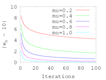
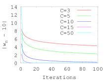
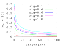
Fig. 1: Performance evaluation of Algorithm 2 with respect to different choices of $\mu$, setting $\gamma_{n}=0.8/n$ and $\sigma=0.01$ (left), with respect to different choices of $C$, with $\gamma_{n}=C/n$, $\mu=0.05$ and $\sigma=0.01$ (center), and with respect to different choices of $\sigma$, for $\mu=0.05$ and $\gamma_{n}=1/n$(right).

5.2 Comparison with other methods

In this section we compare SPG with the SAGE algorithm [28, Algorithm 1] and the FOBOS algorithm in [20]. We note that the main difference between SPG (with $\lambda_{n}=1$ for every $n\in\mathbb{N}^{*}$) and FOBOS is that the latter takes the average of the previous iterates. More precisely the sequence generated by the FOBOS iteration is the following

$$w^{(av)}_{n}=\Big{(}\sum_{k=1}^{n}\eta_{k}\Big{)}^{-1}\sum_{k=1}^{n}\eta_{k}w_{k},\quad\eta_{k}=C_{1}/k,$$ (50)

where $(w_{k})_{k\in\mathbb{N}^{*}}$ is the sequence generated by the SPG algorithm. In [20] it is assumed that the gradient of the smooth term is bounded on the whole space. In our experiments this assumption is not satisfied, but since the sequence of iterates is bounded, the algorithm can be applied and its convergence is guaranteed. One advantage of the SAGE algorithm is that it does require any parameter tuning, since it does not have any free parameter. SPG and FOBOS instead require the choice of the stepsize. We check the accuracy of the three algorithms on different elastic net regularized problems with respect to the number of iterations, since the cost per iteration is basically the same for the three procedures.

5.3 Toy example

We first consider the toy example presented in the previous section (see equation (48)), where we set $\mu=1$. Moreover, we assume that in (49) $s_{n}$ is a realization of a Gaussian random variable with $0$ mean and $0.1$ variance. We run SPG, SAGE, and FOBOS one hundred times for one hundred independent realizations of the random process $(s_{n})_{n\in\mathbb{N}^{*}}$. In SPG, we chose $\gamma_{n}=1/n$, and $\lambda_{n}=1$. Finally, after testing the FOBOS algorithm for different choices of the constant $C_{1}$ defining the stepsize, we got that $\eta_{k}=1/k$ for every $k\in\mathbb{N}^{*}$ gave the best results. The behavior of the sequences $|w_{n}-10|$ corresponding to the three algorithms on the first 1000 iterations is presented in Figure 2. SPG and SAGE have a similar behavior, while FOBOS is slower.

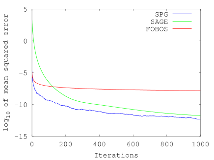
Fig. 2: Convergence of SPG, SAGE, and FOBOS. The performance of SAGE and SPG is comparable, while FOBOS is slower on this example.

5.4 Regression problems with random design

Let $N$ and $p$ be strictly positive integers. Concerning the data generation protocol, the input points $(x_{i})_{1\leq i\leq N}$ are uniformly drawn in the interval $\left[a,b\right]$ (to be specified later in the two cases we consider). For a suitably chosen finite dictionary of real valued functions $(\phi_{k})_{1\leq k\leq p}$ defined on $\left[a,b\right]$, the labels are computed using a noise-corrupted regression function, namely

$$(\forall i\in\{1,\ldots,N\})\quad y_{i}=\sum_{k=1}^{p}\overline{w}_{k}\phi_{k}(x_{i})+\epsilon_{i},$$ (51)

where $(\overline{w_{k}})_{1\leq k\leq p}\in\mathbb{R}^{p}$ and $\epsilon_{i}$ is an additive noise $\epsilon_{i}\sim\mathcal{N}(0,0.3)$.

We will consider two different choices for the dictionary of functions: polynominals, i.e. $(\forall k\in\{1,\ldots,p\})$ $\phi_{k}\colon\left[-1,1\right]\to\mathbb{R}$, $\phi_{k}(x)=x^{k-1}$ and trigonometric functions, i.e. $p=2q+1$ and $(\forall k\in\{1,\ldots,q\})\;\phi_{k}\colon\left[0,2\pi\right]\to\mathbb{R}$, $\phi_{k}(x)=\cos((k-1)x)$ and $(\forall k\in\{q+1,\ldots,2q+1\})\;\phi_{k}\colon\left[0,2\pi\right]\to\mathbb{R}$, $\phi_{k}(x)=\sin(kx)$. The training set and the regression function for the two examples are presented in Figure 3.

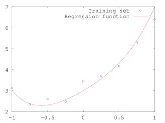
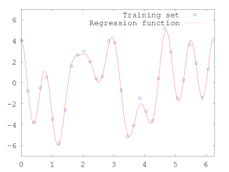
Fig. 3: Left: training set and regression function, on the interval $[-1,1]$ for the polynomial dictionary with $p=6$. Right: training set and regression function on $[0,2\pi]$ for the Fourier basis with $p=21$.

We estimate $\overline{w}$ by solving the following regularized minimization problem

$$\underset{(w_{k})_{1\leq k\leq p}\in\mathbb{R}^{p}}{\text{minimize}}\;\frac{1}{2N}\sum_{i=1}^{N}\Big{(}y_{i}-\sum_{k=1}^{p}w_{k}\phi_{k}(x_{i})\Big{)}^{2}+\frac{1}{2}\sum_{k=1}^{p}(\mu|w_{k}|^{2}+\omega|w_{k}|\big{)},$$ (52)

where $\mu$ and $\omega$ are strictly positive parameters. Problem (52) is a special case of Example 2, and hence it can be solved by using SPG, SAGE, and FOBOS in an incremental fashion. For the polynomial dictionary, we set

$$p=6,\quad N=9,\quad\gamma_{n}=15/(n+100),\quad\eta_{n}=15/(n+100),\quad\mu=0.1,\quad\omega=0.01,$$

$$\overline{w}=[3,2,1,0,1,0].$$ (53)

For the trigonometric dictionary, we set

$$p=21,\quad N=32,\quad\gamma_{n}=\eta_{n}=10/(n+100),\quad\mu=0.01,\quad\omega=0.01,$$

$$\overline{w}=[0,0.2,0,0.5,1,-1,0,1,2,0.5,0,0,-0.1,-2.5,1,0,0,-1,0.9,-0.5,0].$$ (54)

The resulting regression functions using the three algorithms are shown in Figure 4. As can be seen from visual inspection, the three methods provide almost undistinguishable solutions.

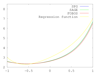
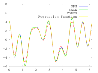
Fig. 4: Regression functions obtained using SPG, SAGE, and FOBOS with polynomial dictionary (left) and trigonometric dictionary (right).

Finally, we computed an approximate solution of (52) by running the forward-backward splitting method in [17] for 50000 iterations. The convergence of the iterations to the solution of (52) is displayed in Figure 5. On the regression problem with the polynomial dictionary, SAGE is performing the best, while on the trigonometric dictionary, SPG is the fastest. The oscillating behavior is mitigated by the averaging procedure at the expanses of a slower convergence rate, as the more regular behaviour of FOBOS clearly shows.

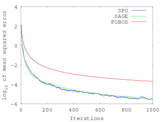
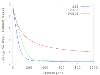
Fig. 5: The convergence of the iterations to the optimal solution of (52) with polynomial dictionary (left) and with trigonometric dictionary (right).

5.5 Deconvolution problems

As a last experiment, we focus on the problem of recovering an ideal signal $\overline{w}$ from a noisy observation of the form

$$\mathbb{R}^{1024}\ni y=h*\overline{w}+s,$$ (55)

where $s\sim\mathcal{N}(0,0.06)$ and $h$ is a Gaussian kernel.

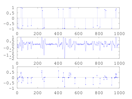
Fig. 6: The ideal signal (top), the noisy signal (middle), and the restored signal (bottom) by SPG.

To find an approximation of the ideal signal, we solve the following variational problem

$$\underset{w\in\mathbb{R}^{1024}}{\text{minimize}}\;T(w),\quad\quad T(w)=\frac{1}{2}\|y-h*w\|^{2}+\|w\|_{1}+\frac{0.02}{2}\|w\|^{2}_{2}.$$ (56)

An approximation $\overline{w}$ of the exact solution is found by running the forward-backward splitting method in [17] for $10000$ iterations. Then, we run SPG, SAGE, and FOBOS with the same initialization, for $5000$ iterations using at the $n$-th iteration a stochastic gradient of the form

$$\mathrm{G}_{n}=\nabla L(w_{n})+s_{n},$$ (57)

where $s_{n}\sim\mathcal{N}(0,0.01)$ and $L(w)=\frac{1}{2}\|y-h*w\|^{2}+\frac{0.02}{2}\|w\|^{2}_{2}$. FOBOS is run with $\eta_{n}=3/(n+100)$. This is not the theoretically optimal choice, but gave better results in practice. In SPG we set $\lambda_{n}=1$ and $\gamma_{n}=3/(n+100)$. Convergence of $(\|w_{n}-\overline{w}\|)_{n\in\mathbb{N}^{*}}$ for the three algorithms is presented in Figure  7. In this case SAGE is the fastest, and SPG shows slightly worse convergence. FOBOS is again slower.

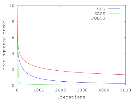
Fig. 7: Convergence of the iterates for SPG, SAGE, and FOBOS with starting point 0.

Finally, we address the problem of the iterations’ sparsity. We generate the data according to the model in (55), starting from an original signal with $993$ zero components. In Figure 8 we display the number of zero components of the iterates. As it can be readily seen by visual inspection, after few iteratons both SAGE ans SPG generate sparse iterations. On this example this does not hold for the FOBOS algorithm, for which the sparsity of the iterates is a decreasing function of the number of iterations. The number of zero components of the last iterate of SPG, SAGE, and FOBOS is 937, 937, and 438, respectively.

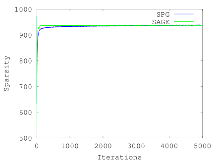
Fig. 8: Number of zero components of the vector $(w_{n}-\overline{w})_{n\in\mathbb{N}^{*}}$ with the same initial point $0$ for SPG and SAGE.

6 Conclusion

In this paper we proposed and studied a stochastic approach to the problem of minimizing a strongly convex non-smooth function. In particular, we have considered the case of composite minimization (the objective function is the sum of a smooth and a convex term) and proposed a stochastic extension of proximal splitting methods which have become widely popular in a deterministic setting. These latter approaches are based on recursively computing the gradient of the smooth term and then applying the proximity operator defined by the convex term. The starting point of the paper is considering the case where only stochastic estimates of the gradient are available. This latter situation is relevant in online approaches to learning and more generally in stochastic and incremental optimization.

The main contributions of this paper are to provide convergence rates in expectation and to establish almost sure convergence of the proposed stochastic proximal gradient method. A further contribution regards our proving techniques, which differ from many previous approaches based on regret analysis and online-to batch conversion. Indeed, our approach is based on extending convex optimization techniques from the deterministic to the stochastic setting. Such extensions are interesting in their own right and could lead to further applications. An outcome of our analysis is that, unlike in the deterministic case, in the stochastic case acceleration does not yield any improvement in the rates.

The analysis in the paper suggests a few venues for future work. A main one is the relaxation of the strong convexity assumption, considering in particular objective functions which are only convex; steps in this direction have been taken in [14]. Deriving high probability, rather than expectation bounds, would also be interesting.

Acknowledgments. This material is based upon work supported by the Center for Brains, Minds and Machines (CBMM), funded by NSF STC award CCF-1231216. L. R. acknowledges the financial support of the Italian Ministry of Education, University and Research FIRB project RBFR12M3AC. S. V. is member of the Gruppo Nazionale per l’Analisi Matematica, la Probabilità e le loro Applicazioni (GNAMPA) of the Istituto Nazionale di Alta Matematica (INdAM).

Appendix A Proofs of auxiliary results

Here we prove the statements about random quasi-Fejér sequences and an upper bound on a numerical sequence satisfying the assumptions of Lemma LABEL:l:ics.

of Proposition 15.

It follows from (33) that

$$(\forall n\in\mathbb{N}^{*})(\forall w\in S)\quad\mathbb{E}[\|w_{n+1}-w\|^{2}]\leq\mathbb{E}[\|w_{n}-w\|^{2}]+\varepsilon_{n}\,.$$ (58)

(i): Since the sequence $(\varepsilon_{n})_{n\in\mathbb{N}^{*}}$ is summable and $\mathbb{E}[\|w-w_{1}\|^{2}]$ is finite, we derive from (58) that $(\mathbb{E}[\|w_{n}-w\|^{2}])_{n\in\mathbb{N}^{*}}$ is a real positive quasi-Fejér sequence, and therefore it converges to some $\zeta_{w}\in\mathbb{R}$ by [13, Lemma 3.1]. Set

$$(\forall n\in\mathbb{N}^{*})\quad r_{n}=\|w_{n}-w\|^{2}+\sum_{k=n}^{\infty}\varepsilon_{n}.$$ (59)

Then, it follows from (33) that

$$(\forall n\in\mathbb{N}^{*})\quad\mathbb{E}[r_{n+1}|\mathcal{A}_{n}] =\mathbb{E}[\|w_{n+1}-w\|^{2}|\mathcal{A}_{n}]+\sum_{k=n+1}^{\infty}\varepsilon_{n}$$

$$\leq\|w_{n}-w\|^{2}+\sum_{k=n}^{\infty}\varepsilon_{n}$$

$$=r_{n}.$$ (60)

Therefore $(r_{n})_{n\in\mathbb{N}}$ is a (real) supermartingale. Since $\sup_{n}\mathbb{E}[\min\{r_{n},0\}]<+\infty$ by (58), $r_{n}$ converges a.s to an integrable random variable [31, Theorem 9.4], that we denote by $\xi_{w}$.

(ii)&(iii): Follow directly by (i). ∎

of Lemma 12.

Note that, for every $m\in\mathbb{N}^{*}$, $n\in\mathbb{N}^{*}$, $m\leq n$:

$$\sum_{k=m}^{n}k^{-\alpha}\geq\varphi_{1-\alpha}(n+1)-\varphi_{1-\alpha}(m),$$ (61)

where $\varphi_{1-\alpha}$ is defined by (10). Since all terms in (18) are positive for $n\geq n_{0}$, by applying the recursion $n-n_{0}$ times we have

$$s_{n+1}\leq s_{n_{0}}\prod_{k=n_{0}}^{n}(1-\eta_{k})+\tau\sum_{k=n_{0}}^{n}\prod_{i=k+1}^{n}(1-\eta_{i})\eta_{k}^{2}.$$ (62)

Let us estimate the first term in the right hand side of (62). Since $1-x\leq\exp(-x)$ for every $x\in\mathbb{R}$, from (61), we derive

$$s_{n_{0}}\prod_{k=n_{0}}^{n}\left(1-\eta_{k}\right)=s_{n_{0}}\prod_{k=n_{0}}^{n}\Big{(}1-\frac{c}{k^{\alpha}}\Big{)} \leq s_{n_{0}}\exp\left(-c\sum_{k=n_{0}}^{n}k^{-\alpha}\right)$$

$$\leq\begin{cases}s_{n_{0}}\big{(}\frac{n_{0}}{n+1}\big{)}^{c}&\text{if $\alpha=1$},\\ \\[-8.61108pt] s_{n_{0}}\exp\Big{(}\frac{c}{1-\alpha}(n_{0}^{1-\alpha}-(n+1)^{1-\alpha})\Big{)}&\text{if $0<\alpha<1$.}\end{cases}$$ (63)

To estimate the second term in the right hand side of (62), let us first consider the case $\alpha<1$, let $m\in\mathbb{N}\setminus\{0\}$ such that $n_{0}\leq n/2\leq m+1\leq(n+1)/2$. We have

$$\sum_{k=n_{0}}^{n}\prod_{i=k+1}^{n} (1-\eta_{i})\eta_{k}^{2}=\sum_{k=n_{0}}^{m}\prod_{i=k+1}^{n}(1-\eta_{i})\eta_{k}^{2}+\sum_{k=m+1}^{n}\prod_{i=k+1}^{n}(1-\eta_{i})\eta_{k}^{2}$$

$$\leq\exp\big{(}-\sum_{i=m+1}^{n}\eta_{i}\big{)}\sum_{k=n_{0}}^{m}\eta_{k}^{2}+{\eta_{m}}\sum_{k=m+1}^{n}\left(\prod_{i=k+1}^{n}(1-\eta_{i})-\prod_{i=k}^{n}(1-\eta_{i})\right)$$

$$=\exp\big{(}-\sum_{i=m+1}^{n}\eta_{i}\big{)}\sum_{k=n_{0}}^{m}\eta_{k}^{2}+{\eta_{m}}\left(1-\prod_{i=m+1}^{n}(1-\eta_{i})\right)$$

$$\leq\exp\big{(}-\sum_{i=m+1}^{n}\eta_{i}\big{)}\sum_{k=n_{0}}^{m}\eta_{k}^{2}+\eta_{m}$$

$$\leq c^{2}\exp\Big{(}\frac{c}{1-\alpha}((m+1)^{1-\alpha}-(n+1)^{1-\alpha})\Big{)}\varphi_{1-2\alpha}(n)+\eta_{m}$$ (64)

$$\leq c^{2}\exp\Big{(}\frac{-ct(n+1)^{1-\alpha}}{1-\alpha}\Big{)}\varphi_{1-2\alpha}(n)+\frac{2^{\alpha}c}{\mu(n-2)^{\alpha}}.$$ (65)

Hence, combining (A) and (65), for $\alpha\in\left]0,1\right[$ we get

$$\quad s_{n+1} \leq\Big{(}\tau c^{2}\varphi_{1-2\alpha}(n)+s_{n_{0}}\exp\Big{(}\frac{cn_{0}^{1-\alpha}}{1-\alpha}\Big{)}\Big{)}\exp\Big{(}\frac{-ct(n+1)^{1-\alpha}}{1-\alpha}\Big{)}+\frac{\tau 2^{\alpha}c}{(n-2)^{\alpha}}.$$ (66)

We next estimate the second term in the right hand side of (62) in the case $\alpha=1$. We have

$$\sum_{k=n_{0}}^{n}\prod_{i=k+1}^{n}(1-\eta_{i})\eta_{k}^{2} =\frac{c^{2}}{(n+1)^{c}}\Big{(}1+\frac{1}{n_{0}}\Big{)}^{c}\sum_{k=n_{0}}^{n}\frac{1}{k^{2-c}}\leq\frac{c^{2}}{(n+1)^{c}}\Big{(}1+\frac{1}{n_{0}}\Big{)}^{c}\varphi_{c-1}(n).$$

Therefore, for $\alpha=1$, we obtain,

$$s_{n+1}\leq s_{n_{0}}\Big{(}\frac{n_{0}}{n+1}\Big{)}^{c}+\frac{\tau c^{2}}{(n+1)^{c}}\Big{(}1+\frac{1}{n_{0}}\Big{)}^{c}\varphi_{c-1}(n),$$ (68)

which completes the proof. ∎

References

• [1] Y. F. Atchade, G. Fort, and E. Moulines. On stochastic proximal gradient algorithms. arXiv:1402.2365, February 2014.
• [2] F. Bach and E. Moulines. Non-asymptotic analysis of stochastic approximation algorithms for machine learning. Proceedings NIPS, 2011.
• [3] K. Barty, J.-S. Roy, and C. Strugarek. Hilbert-valued perturbed subgradient algorithms. Math. Oper. Res., 32(3):551–562, 2007.
• [4] H. H. Bauschke and P. L. Combettes. Convex analysis and monotone operator theory in Hilbert spaces. CMS Books in Mathematics/Ouvrages de Mathématiques de la SMC. Springer, New York, 2011. With a foreword by Hédy Attouch.
• [5] A. Beck and M. Teboulle. A fast iterative shrinkage-thresholding algorithm for linear inverse problems. SIAM J. Imaging Sci., 2(1):183–202, 2009.
• [6] A. Bennar and J.-M. Monnez. Almost sure convergence of a stochastic approximation process in a convex set. Int. J. Appl. Math., 20(5):713–722, 2007.
• [7] A. Benveniste, M. Métivier, and P. Priouret. Adaptive algorithms and stochastic approximations, volume 22 of Applications of Mathematics (New York). Springer-Verlag, Berlin, 1990. Translated from the French by Stephen S. Wilson.
• [8] D. P. Bertsekas. A new class of incremental gradient methods for least squares problems. SIAM Journal on Optimization, 7(4):913–926, 1997.
• [9] D. P. Bertsekas. Incremental gradient, subgradient, and proximal methods for convex optimization: a survey. Optimization for Machine Learning, page 85, 2011.
• [10] D. P. Bertsekas and J. N. Tsitsiklis. Gradient convergence in gradient methods with errors. SIAM J. Optim., 10(3):627–642 (electronic), 2000.
• [11] L. Bottou and Y. Le Cun. On-line learning for very large data sets. Applied Stochastic Models in Business and Industry, 21(2):137–151, 2005.
• [12] Peter Bühlmann and Sara van de Geer. Statistics for high-dimensional data. Springer Series in Statistics. Springer, Heidelberg, 2011. Methods, theory and applications.
• [13] P. L. Combettes. Quasi-Fejérian analysis of some optimization algorithms. In Inherently parallel algorithms in feasibility and optimization and their applications (Haifa, 2000), volume 8 of Stud. Comput. Math., pages 115–152. North-Holland, Amsterdam, 2001.
• [14] P. L. Combettes and J.-C. Pesquet. Stochastic quasi-fejér block-coordinate fixed point iterations with random sweeping, 2014.
• [15] P. L. Combettes and Jean-Christophe Pesquet. Proximal thresholding algorithm for minimization over orthonormal bases. SIAM J. Optim., 18(4):1351–1376, 2007.
• [16] P. L. Combettes and Jean-Christophe Pesquet. Proximal splitting methods in signal processing. In Fixed-point algorithms for inverse problems in science and engineering, volume 49 of Springer Optim. Appl., pages 185–212. Springer, New York, 2011.
• [17] P. L. Combettes and Valérie R. Wajs. Signal recovery by proximal forward-backward splitting. Multiscale Model. Simul., 4(4):1168–1200 (electronic), 2005.
• [18] C. De Mol, E. De Vito, and L. Rosasco. Elastic-net regularization in learning theory. J. Complexity, 25:201–230, 2009.
• [19] O. Devolder. Stochastic first order methods in smooth convex optimization. Technical report, Center for Operations Research and econometrics, 2011.
• [20] J. Duchi and Y. Singer. Efficient online and batch learning using forward backward splitting. J. Mach. Learn. Res., 10:2899–2934, 2009.
• [21] R. Durrett. Probability: theory and examples. Cambridge Series in Statistical and Probabilistic Mathematics. Cambridge University Press, Cambridge, fourth edition, 2010.
• [22] Yu. M. Ermol’ev and A. D. Tuniev. Random fejér and quasi-fejér sequences. Theory of Optimal Solutions– Akademiya Nauk Ukrainskoĭ SSR Kiev, 2:76–83, 1968.
• [23] S. Ghadimi and G. Lan. Optimal stochastic approximation algorithms for strongly convex stochastic composite optimization i: A generic algorithmic framework. SIAM Journal on Optimization, 22(4):1469–1492, 2012.
• [24] E. Hazan, A. Agarwal, and S. Kale. Logarithmic regret algorithms for online convex optimization. Machine Learning, 69(2-3):169–192, 2007.
• [25] E. Hazan and S. Kale. Beyond the regret minimization barrier: an optimal algorithm for stochastic strongly-convex optimization. Journal of Machine Learning Research, 15:2489–2512, 2014.
• [26] A. Juditski and Y. Nesterov. Primal-dual subgradient methods for minimizing uniformly convex functions. arXiv preprint arXiv:1401.1792, 2014.
• [27] A. Juditsky, A. Nemirovski, and C. Tauvel. Solving variational inequalities with stochastic mirror-prox algorithm. Stoch. Syst., 1(1):17–58, 2011.
• [28] J. T. Kwok, C. Hu, and W. Pan. Accelerated gradient methods for stochastic optimization and online learning. In Advances in Neural Information Processing Systems, volume 22, pages 781–789, 2009.
• [29] G. Lan. An optimal method for stochastic composite optimization. Math. Program., 133(1-2, Ser. A):365–397, 2012.
• [30] Q. Lin, X. Chen, and J. Peña. A sparsity preserving stochastic gradient methods for sparse regression. Computational Optimization and Applications, to appear, 2014.
• [31] M. Métivier. Semimartingales, volume 2 of de Gruyter Studies in Mathematics. Walter de Gruyter & Co., Berlin, 1982. A course on stochastic processes.
• [32] J.-M. Monnez. Almost sure convergence of stochastic gradient processes with matrix step sizes. Statist. Probab. Lett., 76(5):531–536, 2006.
• [33] S. Mosci, L. Rosasco, M. Santoro, A. Verri, and S. Villa. Solving structured sparsity regularization with proximal methods. In Machine Learning and Knowledge discovery in Databases European Conference, ECML PKDD 2010, pages 418–433, Barcelona, Spain, 2010. Springer.
• [34] A. Nemirovski, A. Juditsky, G. Lan, and A. Shapiro. Robust stochastic approximation approach to stochastic programming. SIAM J. Optim., 19(4):1574–1609, 2008.
• [35] A. Nemirovski and D. Yudin. Problem Complexity and Method Efficiency in Optimization. Wiley-Intersci. Ser. Discrete Math. 15. John Wiley, New York, 1983.
• [36] Y. Nesterov. Gradient methods for minimizing composite objective function. CORE Discussion Paper 2007/76, Catholic University of Louvain, September 2007.
• [37] B. Polyak. Introduction to Optimization. Optimization Software, New York, 1987.
• [38] B. T. Polyak and A. B. Juditsky. Acceleration of stochastic approximation by averaging. SIAM J. Control Optim., 30(4):838–855, 1992.
• [39] A. Rakhlin, O. Shamir, and K. Sridaran. Making gradient descent optimal for strongly convex stochastic optimization. In Proceedings of the 29th International Conference on Machine Learning, 2012.
• [40] H. Robbins and S. Monro. A stochastic approximation method. Ann. Math. Statistics, 22:400–407, 1951.
• [41] R. T. Rockafellar. Monotone operators and the proximal point algorithm. SIAM J. Control Optimization, 14(5):877–898, 1976.
• [42] M. W. Schmidt, N. Le Roux, and F. Bach. Convergence rates of inexact proximal-gradient methods for convex optimization. In NIPS, pages 1458–1466, 2011.
• [43] S. Shalev-Shwartz, Y. Singer, and N. Srebro. Pegasos: Primal estimated sub-gradient solver for SVM. In Proceedings ICML, 2007.
• [44] S. Shalev-Shwartz and N. Srebro. SVM optimization: inverse dependence on training set size. In Proceedings ICML, 2008.
• [45] O. Shamir and T. Zhang. Stochastic gradient descent for non-smooth optimization: Convergence results and optimal averaging schemes. In Proceedings of the 30th International Conference on Machine Learning, 2013.
• [46] S. Villa, L. Rosasco, S. Mosci, and A. Verri. Proximal methods for the latent group lasso penalty. Comput. Optim. Appl., 58(2):381–407, 2014.
• [47] S. Villa, S. Salzo, L. Baldassarre, and A. Verri. Accelerated and inexact forward-backward algorithms. SIAM J. Optim., 23(3):1607–1633, 2013.
• [48] L. Xiao. Dual averaging methods for regularized stochastic learning and online optimization. J. Mach. Learn. Res., 11:2543–2596, 2010.
• [49] T. Zhang. Multi-stage convex relaxation for learning with sparse regularization. In Advances in Neural Information Processing Systems, pages 1929–1936, 2008.
• [50] M. Zinkevich. Online convex programming and generalized infinitesimal gradient ascent. In Proceedings ICML, 2003.
• [51] Z. Zou and T. Hastie. Regularization and variable selection via the elastic net. Journal of the Royal Statistical Society, Series B, 67:301–320, 2005.