Piecewise linear transformation in diffusive flux discretization

Abstract

To ensure the discrete maximum principle or solution positivity in finite volume schemes, diffusive flux is sometimes discretized as a conical combination of finite differences. Such a combination may be impossible to construct along material discontinuities using only cell concentration values. This is often resolved by introducing auxiliary node, edge, or face concentration values that are explicitly interpolated from the surrounding cell concentrations. We propose to discretize the diffusive flux after applying a local piecewise linear coordinate transformation that effectively removes the discontinuities. The resulting scheme does not need any auxiliary concentrations and is therefore remarkably simpler, while being second-order accurate under the assumption that the structure of the domain is locally layered.

1 Introduction

Diffusion in an anisotropic discontinuous environment plays a role in various fields of engineering, such as subsurface flows. Steady state diffusion of a solute with concentration $C$ in a bounded domain $\Omega\subset\mathbb{R}^{3}$ is modeled by the following boundary problem:

$$\nabla\cdot\mathbf{u}=g,$$ (1)

$$\mathbf{u}=-\mathbb{D}\nabla C,$$ (2)

$$C=g_{\mathrm{D}}\quad\text{on }\Gamma_{\mathrm{D}},$$ (3)

$$\mathbf{u}\cdot\mathbf{n}=g_{\mathrm{N}}\quad\text{on }\Gamma_{\mathrm{N}},$$ (4)

$$\mathbf{u}\cdot\mathbf{n}=\Psi(C-g_{\mathrm{R}})\quad\text{on }\Gamma_{\mathrm{R}},$$ (5)

where $\mathbf{u}$ is the velocity, $g$ is the volumetric source term, $\mathbf{n}$ is the unit vector normal to $\partial\Omega$ pointing outward, $\Psi$ is the transfer coefficient, $\Gamma_{\mathrm{D}}\cup\Gamma_{\mathrm{R}}=\overline{\Gamma_{\mathrm{D}}\cup\Gamma_{\mathrm{R}}}$, $\Gamma_{\mathrm{D}}\cup\Gamma_{\mathrm{N}}\cup\Gamma_{\mathrm{R}}=\partial\Omega$, $\Gamma_{\mathrm{D}}\cup\Gamma_{\mathrm{R}}\neq\emptyset$, and $\Gamma_{\mathrm{D}}$, $\Gamma_{\mathrm{N}}$, and $\Gamma_{\mathrm{R}}$ are mutually disjoint. Diffusion tensor $\mathbb{D}$ is symmetric, positive definite, and piecewise continuous. Connected subsets of $\Omega$ in which $\mathbb{D}$ is continuous are called material zones, and the interfaces between them are referred to as material interfaces. Presumably, mesh faces coincide with material interfaces, i.e. $\mathbb{D}$ is continuous within mesh cells.

Various numerical schemes are used to solve this problem. Most of them produce non-physical oscillations and negative concentration values in particular cases. Nevertheless, certain schemes are specifically designed to address these issues. One such finite volume scheme appeared in [1] and was further developed in [2, 3, 4, 5, 6, 7, 8, 9]. These schemes do not satisfy the maximum principle, but they guarantee that the concentration does not become negative.

In addition to the primary concentration unknowns associated with mesh cells, these schemes use auxiliary concentration values located in faces and elsewhere. Face concentration values are easily determined from the continuity, but some kind of interpolation must be used to determine other auxiliary values. The interpolation method presented in [7] performs this task using piecewise linear interpolation and convex combinations. It satisfies the maximum principle and is second order accurate even when it uses interpolation nodes at the opposite sides of a material discontinuity. Since a simple brute force search for collocation points that form a convex combination can result in a combinatorial explosion, in [7] we proposed a complex but efficient alternative search algorithm based on Delaunay triangulations.

In this paper we deploy the piecewise linear transformation introduced in [7] directly in the velocity decomposition, without any auxiliary concentration variables. Such a scheme is simpler than [7] because the complicated construction of convex combinations is avoided. In addition, fluxes over discontinuities do not need special treatment, resulting in further simplification.

The paper is organized as follows: in §2 we explain how to use the piecewise linear transformation to obtain a one-side flux approximation. In §3 the one-side fluxes are combined in the usual fashion to obtain a two-point scheme. Euler implicit temporal discretization of the time-dependent problem is presented in §4. Numerical tests presented in §5 show that the accuracy and the convergence rate do not change much in comparison to [7], and thus the simpler scheme should be the method of choice. Moreover, it is shown that a single iteration is sufficient to maintain the second order accuracy in a time-dependent problem.

2 Fluxes and piecewise linear transformation

The piecewise linear transformation used here to approximate the flux was constructed in [7]. The main steps are repeated for convenience.

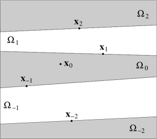
Figure 1: It is assumed that the structure of the domain is locally layered.

We assume that some neighborhood of point $\mathbf{x}_{0}\in\Omega$ consists of layers $\Omega_{-m}$, $\dots$, $\Omega_{n}$, $m\geq 0$, $n\geq 0$, with interfaces that are either planes or approximated by planes (see Fig. 1). The diffusion tensor is allowed to have discontinuities between layers, but it is assumed to be constant or almost constant within each layer, thus $\mathbb{D}|_{\Omega_{i}}=\mathbb{D}_{i}$. This assumption needs to hold only locally — the diffusion tensor is allowed to vary smoothly within layers on a larger scale. We assume that the concentration changes linearly in each layer

$$C(\mathbf{x})=C_{i}+\mathbf{G}_{i}\cdot(\mathbf{x}-\mathbf{x}_{i}),\qquad\mathbf{x}_{i}\in\overline{\Omega}_{i}.$$ (6)

This function must satisfy two conditions:

1. It must be continuous, and

2. The flux through each interface must be continuous.

The two conditions eliminate all but four degrees of freedom in the piecewise linear function $C(\mathbf{x})$, which may be written as

$$C(\mathbf{x})=C_{0}+\mathbf{G}_{0}\cdot F(\mathbf{x}),$$ (7)

where $F:\mathbb{R}^{3}\rightarrow\mathbb{R}^{3}$ is a piecewise linear transformation depending on the diffusion tensors and geometry but not on the concentration. In [7] we derived explicit formulas to compute $F$.

In [7] we evaluate (7) to obtain the concentration values at points. In contrast, in this paper (7) is not evaluated at points: instead, the gradient of (7) is used to approximate the normal velocity component $\mathbf{n}_{f}\cdot\mathbf{u}$ in some mesh face $f$. We assume that this face belongs to cell $T$ and that $\mathbf{n}_{f}$ points outside from this cell. For point $\mathbf{x}_{0}$ in (6) we take the centroid $\mathbf{x}_{T}$; thus $C_{0}=C_{T}$ in (7). We need to determine the three components of $\mathbf{G}_{0}$. These are found by solving a linear system consisting of three equations of the following types:

$$F(\mathbf{x}_{\mathcal{T}})\cdot\mathbf{G}_{0}=C_{\mathcal{T}}-C_{T}\quad\text{if }\mathcal{T}\text{ is a mesh cell,}$$ (8)

$$F(\mathbf{x}_{n})\cdot\mathbf{G}_{0}=g_{\mathrm{D}}(\mathbf{x}_{n})-C_{T}\quad\text{if }\mathbf{x}_{n}\text{ is a node in }\Gamma_{\mathrm{D}},$$ (9)

$$F(\mathbf{x}_{f})\cdot\mathbf{G}_{0}=g_{\mathrm{D}}(\mathbf{x}_{f})-C_{T}\quad\text{if }f\text{ is a face in }\Gamma_{\mathrm{D}},$$ (10)

$$\mathbf{n}_{f}^{\mathrm{T}}\mathbb{D}(\mathbf{x}_{f})\nabla F(\mathbf{x}_{f})\mathbf{G}_{0}=-g_{\mathrm{N}}(\mathbf{x}_{f})\quad\text{if }f\text{ is a face in }\Gamma_{\mathrm{N}},$$ (11)

$$\left(F(\mathbf{x}_{f})+\frac{1}{\Psi}\mathbf{n}_{f}^{\mathrm{T}}\mathbb{D}(\mathbf{x}_{f})\nabla F(\mathbf{x}_{f})\right)\cdot\mathbf{G}_{0}=g_{\mathrm{R}}(\mathbf{x}_{f})-C_{T}\quad\text{if }f\text{ is a face in }\Gamma_{\mathrm{R}}.$$ (12)

Point $\mathbf{x}_{f}$ is the centroid of face $f$. The last equation follows from

$$-\mathbf{n}_{f}^{\mathrm{T}}\mathbb{D}(\mathbf{x}_{f})\nabla F(\mathbf{x}_{f})\mathbf{G}_{0}=\Psi(C_{T}+\mathbf{G}_{0}\cdot F(\mathbf{x}_{f})-g_{\mathrm{R}}(\mathbf{x}_{f}))$$ (13)

and may be written in a form similar to (9) and (10):

$$F\left(\mathbf{x}_{f}+\frac{1}{\Psi}\mathbb{D}(\mathbf{x}_{f})\mathbf{n}_{f}\right)\cdot\mathbf{G}_{0}=g_{\mathrm{R}}(\mathbf{x}_{f})-C_{T}\quad\text{if }f\text{ is a face in }\Gamma_{\mathrm{R}}.$$ (14)

Three equations of the form (8)–(12) constitute a linear system

$$M\mathbf{G}_{0}=\mathbf{r}.$$ (15)

If this system has a unique solution $\mathbf{G}_{0}=M^{-1}\mathbf{r}$, then the normal velocity component at face $f$ can be approximated as

$$\mathbf{n}_{f}\cdot\mathbf{u}\approx-\mathbf{n}_{f}^{\mathrm{T}}\mathbb{D}(\mathbf{x}_{f})M^{-1}\mathbf{r}=-\boldsymbol{\alpha}\cdot\mathbf{r}$$ (16)

because $f\subset\overline{\Omega}_{0}$ and $\nabla F\equiv I$ in $\Omega_{0}$. Coefficient vector $\boldsymbol{\alpha}$ is determined by solving

$$M^{\mathrm{T}}\boldsymbol{\alpha}=\mathbb{D}(\mathbf{x}_{f})\mathbf{n}_{f}.$$ (17)

Equations that make up the system (15) are chosen in such a way that the obtained coefficients $\boldsymbol{\alpha}$ are non-negative. The search for these equations is performed by testing all combinations of neighboring cells and boundary conditions belonging to the candidate set, in the same way that the brute force strategy in [7] works. The candidate set is initialized with cell $T$, cells that share a face with $T$, boundary faces of $T$ and Dirichlet boundary nodes of $T$. If equations leading to non-negative $\boldsymbol{\alpha}$ are not found, the candidate set is extended by adding all neighboring cells, boundary faces and Dirichlet boundary nodes of the current member cells, until non-negative $\boldsymbol{\alpha}$ is obtained.

If matrix $M$ in (15) is ill-conditioned, this typically results in large coefficients $\boldsymbol{\alpha}$. The resulting interpolation is inaccurate, so the combination is discarded if some $\alpha_{i}\|\mathbf{t}_{i}\|/\|\mathbb{D}\mathbf{n}_{f}\|$ is larger than a suitably chosen value $A_{\text{max}}$ discussed in the next section, where $\mathbf{t}_{i}$ is the vector multiplying $\mathbf{G}_{0}$ in the corresponding equation (8)–(12).

If more than one conical combination is found, we apply a strategy similar to the one used in [2]: starting with combinations containing the cell that shares the face $f$ with the cell $T$, we choose the first encountered conical combination such that $\max_{i}(\alpha_{i}m_{i})/\|\mathbb{D}(\mathbf{x}_{f})\mathbf{n}_{f}\|_{2}\leq 1$, where $m_{i}$ is the 2-norm of the $i^{\text{th}}$ row of matrix $M$. If no such combination is encountered, then we choose the one for which this ratio is minimal.

2.1 Alternative: harmonic averaging points

Let points $\mathbf{x}_{1}$ and $\mathbf{x}_{2}$ be separated by a material interface. The same two conditions leading to transformation $F$ were used in [10] to compute the concentration at a suitably chosen point at the interface as a convex combination of concentration values at $\mathbf{x}_{1}$ and $\mathbf{x}_{2}$. Such so-called harmonic averaging point can be used in (8) in the place of $\mathcal{T}$, as an alternative to transformation $F$. The two approaches are equivalent under certain conditions:

• Either $\mathbf{x}_{1}$ or $\mathbf{x}_{2}$ is equal to $\mathbf{x}_{T}$;

• The concentration at the harmonic averaging point is evaluated implicitly;

• Points $\mathbf{x}_{1}$ and $\mathbf{x}_{2}$ are in neighboring layers;

• Neumann and Robin boundary conditions in faces not belonging to $\overline{\Omega}_{0}$ are not used in (15).

The notion of harmonic averaging points could be extended to interpolate over multiple layers and to deploy boundary conditions in a similar way this is done here.

3 Non-linear two-point scheme

As usual, finite volume discretization is performed applying the divergence theorem to the integral of (1) over the mesh cell $T$:

$$\oint_{T}\mathbf{u}\cdot\mathbf{n}{\rm d}S=\sum_{f}\chi_{T,f}u_{f}=\int_{T}g{\rm d}T,\qquad u_{f}=\int_{f}\mathbf{u}\cdot\mathbf{n}{\rm d}S,$$ (18)

where $\mathbf{n}_{f}$ is the fixed unit normal vector associated with face $f$, and $\chi_{T,f}=1$ if $\mathbf{n}_{f}$ points outside of $T$, or $\chi_{T,f}=-1$ otherwise.

The two-point scheme is constructed in a similar way as in [2, 6], but simpler because the discontinuities do not need to be treated separately. Approximation (16) can be written as

$$\mathbf{n}_{f}\cdot\mathbf{u}\approx\sum_{i}\alpha_{i}(C_{T}-C_{i})+\sum_{j}\alpha_{j}g_{\mathrm{N}}(\mathbf{x}_{j}).$$ (19)

The convex combination of such expressions that correspond to the cells $T^{+}$ and $T^{-}$ sharing the internal face $f$

$$\frac{u_{f}}{|f|}\approx\mu_{+}\left(\sum_{i}\alpha_{i}^{+}(C_{+}-C^{+}_{i})+\sum_{j}\alpha_{j}^{+}g_{\mathrm{N}}(\mathbf{x}_{j}^{+})\right)-\mu_{-}\left(\sum_{k}\alpha_{k}^{-}(C_{-}-C^{-}_{i})+\sum_{l}\alpha_{l}^{-}g_{\mathrm{N}}(\mathbf{x}_{l}^{-})\right)$$ (20)

is chosen in such a way that the contributions of concentration values other than $C_{+}$ and $C_{-}$ cancel, together with the contributions of inflow Neumann faces. Here $C_{\pm}$ denotes the concentration in cell $T^{\pm}$. Thus weights $\mu_{+}$ and $\mu_{-}$ are determined such that

$$\mu_{+}+\mu_{-}=1,\qquad-\mu_{+}d_{+}+\mu_{-}d_{-}=0,$$ (21)

where

$$d_{\pm}=\sum_{\begin{subarray}{c}i\\ \mathbf{x}_{i}\neq\mathbf{x}_{\mp}\end{subarray}}\alpha_{i}C_{i}^{\pm}-\sum_{\begin{subarray}{c}j\\ g_{\mathrm{N}}(\mathbf{x}_{j}^{\pm})<0\end{subarray}}\alpha_{j}^{\pm}g_{\mathrm{N}}(\mathbf{x}_{j}^{\pm}).$$ (22)

If $d_{+}+d_{-}\neq 0$, then

$$\mu_{+}=\frac{d_{-}}{d_{+}+d_{-}},\qquad\mu_{-}=\frac{d_{+}}{d_{+}+d_{-}}.$$ (23)

Otherwise we take $\mu_{\pm}=\tfrac{1}{2}$.

In this way flux approximation (20) reduces to a two-point formula

$$u_{f}\approx M_{f}^{+}C_{+}-M_{f}^{-}C_{-}+r_{f},$$ (24)

where

$$M_{f}^{\pm}=|f|\left(\mu_{\pm}\sum_{i}\alpha_{i}^{\pm}+\mu_{\mp}\sum_{\begin{subarray}{c}k\\ \mathbf{x}_{k}=\mathbf{x}_{\pm}\end{subarray}}\alpha_{k}^{\mp}\right),\qquad r_{f}=|f|\left(\mu_{+}\sum_{j}\alpha_{j}^{+}g_{\mathrm{N}}(\mathbf{x}_{j}^{+})-\mu_{-}\sum_{l}\alpha_{l}^{-}g_{\mathrm{N}}(\mathbf{x}_{l}^{-})\right).$$ (25)

Fluxes through Dirichlet faces are discretized in the same way as in [2, 6], treating the boundary face as a flat cell of zero volume. The same technique is applied to Robin faces by treating the Robin condition at $\mathbf{x}_{f}$ as a Dirichlet condition specified at $\mathbf{x}_{f}+\tfrac{1}{\Psi}\mathbb{D}(\mathbf{x}_{f})\mathbf{n}_{f}$ (see (14)).

Experiments have shown that it is better to accept relatively large coefficients $\boldsymbol{\alpha}$ than to extend the candidate set, which also increases the error due to the increased distances between points. From (22) and (23) we see that large coefficients in a one-side flux cause the weight assigned to this flux to be small and the weight assigned to the opposite flux to be large. In this way the influence of inaccurate interpolation vanishes. Owing to this fortunate circumstance, we only discard combinations if $\alpha_{i}\|\mathbf{t}_{i}\|/\|\mathbb{D}\mathbf{n}_{f}\|$ is larger than $A_{\text{max}}=1000$ for some $i$.

Finite volume discretization with fluxes as in (24) results in a non-linear system $A(\mathbf{C})\mathbf{C}=\mathbf{b}(\mathbf{C})$, where vector $\mathbf{C}$ contains concentration values in all cells.

Starting with some $\mathbf{C}^{0}$, consecutive iterations are computed by solving the linearized system $A(\mathbf{C}^{n})\mathbf{C}^{n+1}=\mathbf{b}(\mathbf{C}^{n})$ until the convergence criterion

$$\frac{\|A(\mathbf{C}^{n})\mathbf{C}^{n}-\mathbf{b}(\mathbf{C}^{n})\|}{\|\mathbf{b}(\mathbf{C}^{n})\|}<\varepsilon$$ (26)

is met.

If $\mathbf{C}^{n}$ is non-negative, then $A(\mathbf{C}^{n})$ is an M-matrix because coefficients $M^{\pm}_{f}$ in (24) are non-negative, which follows from the non-negativity of $d_{\pm}$, (23), and (25). In the absence of Neumann outflow boundaries and if $g_{\mathrm{D}}\geq 0$ and $g_{\mathrm{R}}\geq 0$, the right-hand side is non-negative. Therefore $\mathbf{C}^{n+1}$ is non-negative as well, and by induction the concentration is non-negative in each iteration.

4 Time-dependent problem

A transient problem is obtained by adding a time derivative to the continuity equation (1):

$$\frac{\partial C}{\partial t}+\nabla\cdot\mathbf{u}=g$$ (27)

when $t>t_{0}$. For this equation to have a unique solution, in addition to boundary conditions (3)-(5), one also needs to specify an initial condition $C|_{t=t_{0}}=C_{0}$. Condition $\Gamma_{\mathrm{D}}\cup\Gamma_{\mathrm{R}}\neq\emptyset$ is no longer necessary.

Using Euler implicit discretization, we obtain

$$|T|\frac{C_{T}^{n+1}-C_{T}^{n}}{\Delta t^{n+1}}+\sum_{f}\chi_{T,f}\left(M_{f}^{+,n+1}C_{+}^{n+1}-M_{f}^{-,n+1}C_{-}^{n+1}+r_{f}^{n+1}\right)=\int_{T}g^{n+1}{\rm d}T$$ (28)

in the place of (18), where $\Delta t$ is the time step and the last superscript indicates the time level.

At each time level this non-linear system is solved using Picard linearization

$$|T|\frac{C_{T}^{n+1,m+1}-C_{T}^{n}}{\Delta t^{n+1}}+\sum_{f}\chi_{T,f}\left(M_{f}^{+,n+1,m}C_{+}^{n+1,m+1}-M_{f}^{-,n+1,m}C_{-}^{n+1,m+1}+r_{f}^{n+1,m}\right)=\int_{T}g^{n+1,m}{\rm d}T,$$ (29)

where the superscript after the time level indicates the iteration number.

To preserve the second-order accuracy, one must take $\Delta t=\mathcal{O}(h^{2})$, where mesh parameter $h$ is proportional to the longest edge length.

Inspired by [11, 12, 13], for the initial approximation we take

$$C_{T}^{n+1,0}=\max(C_{T}^{n}+\Delta t^{n+1}\dot{C}_{T}^{n},0),\qquad\dot{C}_{T}^{n}=\frac{C_{T}^{n}-C_{T}^{n-1}}{\Delta t^{n}}.$$ (30)

Such an initial value violates the mass conservation property, but it is used only to compute coefficients $M_{f}^{\pm}$ in the first iteration. The conservation and positivity of subsequent iterations follow from the matrix structure. Moreover, since the error of the initial value is already $\mathcal{O}(\Delta t^{2})$, a single iteration in each time step is enough to maintain the $\mathcal{O}(\Delta t)=\mathcal{O}(h^{2})$ accuracy at the end of the time stepping process.

Extrapolation (30) cannot be used in the first time step because $\dot{C}_{T}^{0}$ is not known. It is suggested in [11, 12, 13] to calculate $\dot{C}_{T}^{0}$ from the truncation error obtained by substituting the initial solution into the stationary problem. However, finite volume schemes are inconsistent in the finite difference sense so $\dot{C}_{T}^{0}$ obtained in this way is inaccurate. One can take $C^{1,0}_{T}=C^{0}_{T}$ instead. If a single iteration is performed, the error $\mathcal{O}(\Delta t)$ is introduced only at the first time step while all other steps add $\mathcal{O}(\Delta t^{2})$, so the total error is still $\mathcal{O}(\Delta t)$. Alternatively, one may compute a few iterations in the first time step.

5 Examples

The following examples demonstrate that, on average, the proposed scheme is not less accurate and does not require more iterations than the more complicated version presented in [7].

We report the numbers of iterations $n_{6}$ and $n_{9}$ until convergence is achieved with $\varepsilon=10^{-6}$ and $\varepsilon=10^{-9}$, respectively. Linear systems are solved using the BiCGStab solver with an accuracy of $10^{-12}$.

The following norms are used to quantify the concentration and flux errors:

$$\varepsilon^{C}_{2}=\left[\frac{\sum_{T}(C(\mathbf{x}_{T})-C_{T})^{2}|T|}{\sum_{T}(C(\mathbf{x}_{T}))^{2}|T|}\right]^{1/2},\quad\varepsilon_{\text{max}}^{C}=\frac{\max_{T}|C(\mathbf{x}_{T})-C_{T}|}{\left[\sum_{T}(C(\mathbf{x}_{T}))^{2}|T|/\sum_{T}|T|\right]^{1/2}},$$

$$\varepsilon^{\mathbf{u}}_{2}=\left[\frac{\sum_{f}(\mathbf{u}(\mathbf{x}_{f})-u_{f}/|f|)^{2}|f|}{\sum_{f}(\mathbf{u}(\mathbf{x}_{f})\cdot\mathbf{n}_{f})^{2}|f|}\right]^{1/2},\quad\varepsilon^{\mathbf{u}}_{\text{max}}=\frac{\max_{f}|\mathbf{u}(\mathbf{x}_{f})\cdot\mathbf{n}_{f}-u_{f}/|f||}{\left[\sum_{f}(\mathbf{u}(\mathbf{x}_{f})\cdot\mathbf{n}_{f})^{2}|f|/\sum_{f}|f|\right]^{1/2}},$$ (31)

where $C_{T}$ is the computed concentration in cell $T$, $u_{f}$ is the computed flux through face $f$, and $C(\mathbf{x})$ and $\mathbf{u}(\mathbf{x})$ are the exact concentration and velocity functions, respectively.

Example 1

This is a modified version of an example that appeared in [2]. The domain is the unit cube. The diffusion tensor is

$$\mathbb{D}=\left\{\begin{array}[]{c}\mathbb{D}_{1}\quad\text{if }x<0.5\\ \mathbb{D}_{2}\quad\text{otherwise}\end{array}\right.,\quad\mathbb{D}_{1}=\left[\begin{array}[]{c c c}3&1&0\\ 1&3&0\\ 0&0&1\end{array}\right],\quad\mathbb{D}_{2}=\left[\begin{array}[]{c c c}10&3&0\\ 3&1&0\\ 0&0&1\end{array}\right].$$ (32)

The source term is chosen such that the exact solution is

$$C=\left\{\begin{array}[]{c}1-2y^{2}+4xy+2y+6x\quad\text{if }x<0.5,\\ 3.5-2y^{2}+2xy+x+3y\quad\text{otherwise.}\end{array}\right.$$ (33)

The exact concentration is set at $z=0$ and $z=1$, the exact flux is specified at $y=0$ and $y=1$, and the Robin condition is prescribed at $x=0$ and $x=1$. We take $g_{\mathrm{R}}|_{x=0}\equiv 0$ and $g_{\mathrm{R}}|_{x=1}\equiv 10$, while $\Psi$ is chosen so (33) is the solution.

This problem was solved on three types of meshes: cubic, triangular prismatic, and tetrahedral. The errors and iteration numbers given in Table 1 show that there is little difference in the accuracy and convergence rate, compared with the previous version of the scheme [7].

	Current scheme				Previous scheme
$h$	1/10	1/20	1/40	1/80	1/10	1/20	1/40	1/80
Hexahedral grids
$\varepsilon_{2}^{c}$	7.64e-4	1.98e-4	5.09e-5	1.31e-5	7.15e-4	1.91e-4	4.97e-5	1.25e-5
$\varepsilon_{\text{max}}^{c}$	3.12e-3	9.88e-4	3.08e-4	9.43e-5	3.00e-3	1.44e-3	5.90e-4	2.19e-4
$\varepsilon_{2}^{\mathbf{u}}$	4.53e-3	1.89e-3	7.40e-4	2.76e-4	3.89e-3	1.48e-3	5.46e-4	1.98e-4
$\varepsilon_{\text{max}}^{\mathbf{u}}$	2.88e-2	1.71e-2	9.18e-3	4.61e-3	1.85e-2	9.94e-3	5.07e-3	2.60e-3
$n_{6}$	28	52	81	107	38	62	87	115
$n_{9}$	45	84	143	205	61	100	154	220
Prismatic grids
$\varepsilon_{2}^{c}$	4.78e-4	1.05e-4	2.48e-5	5.64e-6	4.41e-4	9.74e-5	2.31e-5	5.49e-6
$\varepsilon_{\text{max}}^{c}$	4.87e-3	2.25e-3	6.68e-4	2.95e-4	3.92e-3	1.68e-3	5.27e-4	2.17e-4
$\varepsilon_{2}^{\mathbf{u}}$	4.04e-3	2.21e-3	1.15e-3	5.84e-6	3.92e-3	2.16e-3	1.14e-3	5.83e-4
$\varepsilon_{\text{max}}^{\mathbf{u}}$	4.31e-2	2.35e-2	1.38e-2	7.74e-3	2.81e-2	1.55e-2	8.10e-3	4.50e-3
$n_{6}$	39	65	88	110	50	72	95	117
$n_{9}$	63	112	164	230	82	126	179	240
Tetrahedral grids
$\varepsilon_{2}^{c}$	5.70e-4	1.41e-4	2.94e-5	7.45e-6	6.83e-4	1.65e-4	3.20e-5	7.42e-6
$\varepsilon_{\text{max}}^{c}$	6.15e-3	2.32e-3	7.59e-4	2.61e-4	8.96e-3	4.30e-3	1.02e-3	3.68e-4
$\varepsilon_{2}^{\mathbf{u}}$	5.15e-3	2.37e-3	1.15e-3	5.59e-4	5.06e-3	2.37e-3	1.15e-3	5.58e-4
$\varepsilon_{\text{max}}^{\mathbf{u}}$	3.47e-2	1.49e-2	8.18e-3	2.61e-3	3.15e-2	2.09e-2	8.17e-3	6.03e-3
$n_{6}$	96	159	220	279	97	158	226	290
$n_{9}$	147	260	384	534	150	259	393	549

Table 1: Errors and iteration numbers in Example 1.

Example 2

This is a modified version of an example used in [7]. The domain is again a unit cube. The diffusion tensor is

$$\mathbb{D}=(1+0.25\cos(x+y-z))\cdot\left\{\begin{array}[]{c}\mathbb{D}_{1}\quad\text{if }x<0.5\\ \mathbb{D}_{2}\quad\text{otherwise,}\end{array}\right.$$ (34)

$$\mathbb{D}_{1}=\left[\begin{array}[]{c c c}1&0&0\\ 0&1&0\\ 0&0&1\end{array}\right],\quad\mathbb{D}_{2}=\left[\begin{array}[]{c c c}100&0&0\\ 0&0.01&0\\ 0&0&1\end{array}\right].$$ (35)

The source term is chosen such that the exact solution is

$$C=\left\{\begin{array}[]{c}\cos(\pi x)\sin(\pi y)+1\quad\text{if }x<0.5,\\ 0.01\cos(\pi x)\sin(\pi y)+1\quad\text{otherwise.}\end{array}\right.$$ (36)

The exact concentration is prescribed at $x=1$, $y=0$, and $y=1$, and the exact flux is specified elsewhere. Table 2 shows the errors and iteration numbers.

	Current scheme				Previous scheme
$h$	1/10	1/20	1/40	1/80	1/10	1/20	1/40	1/80
Hexahedral grids
$\varepsilon_{2}^{c}$	2.39e-3	5.98e-4	1.49e-4	3.73e-5	5.28e-3	1.04e-3	2.17e-4	5.34e-5
$\varepsilon_{\text{max}}^{c}$	6.66e-3	1.69e-3	4.25e-4	1.06e-4	3.22e-2	8.07e-3	2.94e-3	7.78e-4
$\varepsilon_{2}^{\mathbf{u}}$	4.21e-3	1.05e-3	2.62e-4	6.56e-5	3.14e-2	1.08e-2	3.56e-3	1.46e-3
$\varepsilon_{\text{max}}^{\mathbf{u}}$	1.28e-2	3.20e-3	7.99e-4	1.99e-4	2.79e-1	1.60e-1	8.50e-2	4.13e-2
$n_{6}$	1	1	1	1	2	4	4	4
$n_{9}$	1	1	1	1	4	6	7	7
Prismatic grids
$\varepsilon_{2}^{c}$	1.43e-3	3.58e-4	8.92e-5	2.12e-5	3.53e-3	8.05e-4	1.51e-4	3.13e-5
$\varepsilon_{\text{max}}^{c}$	5.53e-3	1.78e-3	4.18e-4	1.07e-4	2.36e-2	8.21e-3	2.05e-3	5.19e-4
$\varepsilon_{2}^{\mathbf{u}}$	4.90e-3	1.26e-3	3.96e-4	1.92e-4	2.80e-2	1.07e-2	3.63e-3	1.31e-3
$\varepsilon_{\text{max}}^{\mathbf{u}}$	5.77e-2	2.03e-2	1.22e-2	8.82e-3	3.79e-1	2.06e-1	1.02e-1	5.36e-2
$n_{6}$	6	8	11	17	6	8	11	16
$n_{9}$	10	15	22	36	10	14	21	35
Tetrahedral grids
$\varepsilon_{2}^{c}$	1.03e-3	1.74e-4	3.45e-5	7.08e-6	1.02e-3	1.74e-4	3.48e-5	7.10e-6
$\varepsilon_{\text{max}}^{c}$	1.21e-2	1.50e-3	3.92e-4	9.44e-5	1.23e-2	1.50e-3	4.00e-4	1.02e-4
$\varepsilon_{2}^{\mathbf{u}}$	2.49e-2	8.98e-3	4.19e-3	1.99e-3	2.31e-2	8.56e-3	4.09e-3	1.96e-3
$\varepsilon_{\text{max}}^{\mathbf{u}}$	2.02e-1	1.49e-1	6.59e-2	4.21e-2	2.03e-1	1.01e-1	4.62e-2	2.53e-2
$n_{6}$	54	88	147	231	56	89	154	239
$n_{9}$	91	164	313	571	94	166	323	579

Table 2: Errors and iteration numbers in Example 2.

In this example the scheme reduces to a linear one on structured grids, therefore convergence is achieved in a single iteration. This was not the case with scheme [7], owing to the treatment of Dirichlet boundary conditions. The change also results in smaller errors on structured and prismatic grids. This is only possible because the anisotropy axes are aligned with the grid, which was not the case in the previous example.

The present example was also solved on Kershaw meshes [14]. The errors and iteration numbers are shown in Table 3. No more than one candidate set extension was necessary to find the cells and boundary conditions that give non-negative coefficients $\boldsymbol{\alpha}$ in (16), in comparison to [7] where up to 11 extension rounds were necessary to find convex combinations on the same meshes. As explained in [7], to find a convex combination for a mesh node that does not belong to the convex hull of nearby collocation points, a large number of extensions is necessary. Kershaw grids contain such nodes. On the other hand, the new scheme does not use interpolated point values so it does not suffer from this problem.

	Current scheme
$h$	1/8	1/16	1/32	1/64	1/128
$\varepsilon_{2}^{c}$	2.38e-2	2.08e-2	1.44e-2	6.62e-3	2.21e-3
$\varepsilon_{\text{max}}^{c}$	1.21e-1	9.32e-2	6.06e-2	2.85e-2	9.21e-3
$\varepsilon_{2}^{\mathbf{u}}$	3.67e-1	2.55e-1	1.52e-1	7.56e-2	2.95e-2
$\varepsilon_{\text{max}}^{\mathbf{u}}$	2.52	1.92	9.04e-1	5.58e-1	3.21e-1
$n_{6}$	59	118	203	381	635
$n_{9}$	91	186	331	670	1239
	Previous scheme
$\varepsilon_{2}^{c}$	2.11e-1	2.07e-2	1.44e-2	6.62e-3	2.21e-3
$\varepsilon_{\text{max}}^{c}$	7.91e-1	9.38e-2	6.06e-2	2.84e-2	9.21e-3
$\varepsilon_{2}^{\mathbf{u}}$	5.51e-1	2.41e-1	1.52e-1	7.51e-2	2.93e-2
$\varepsilon_{\text{max}}^{\mathbf{u}}$	3.90	1.42	8.37e-1	5.34e-1	3.13e-1
$n_{6}$	63	118	206	384	636
$n_{9}$	97	199	335	674	1241

Table 3: Errors and iteration numbers on Kershaw grids in Example 2.

Example 3

The diffusion tensor is

$$\mathbb{D}=\left\{\begin{array}[]{c c }\mathbb{D}_{1}&\text{if }x<0.1\\ \mathbb{D}_{2}&\text{if }x<0.95-0.75y\\ \mathbb{D}_{3}&\text{otherwise,}\end{array}\right.$$ (37)

$$\mathbb{D}_{1}=\left[\begin{array}[]{c c c}3&1&0\\ 1&3&0\\ 0&0&1\end{array}\right],\quad\mathbb{D}_{2}=\left[\begin{array}[]{c c c}10&3&0\\ 3&1&0\\ 0&0&1\end{array}\right],\quad\mathbb{D}_{3}=\left[\begin{array}[]{c c c}1.2&1&0\\ 1&2&0\\ 0&0&1\end{array}\right].$$ (38)

The exact concentration is a piecewise linear function

$$C=\left\{\begin{array}[]{c c}1+6x+4y&\text{if }x<0.1\\ 1.5+7x+4y&\text{if }x<0.95-0.75y\\ -2.3+5x+7y&\text{otherwise.}\end{array}\right.$$ (39)

The exact concentration is set at $z=0$ and $z=1$, the exact flux is specified at $y=0$ and $y=1$, while the Robin condition is set elsewhere with $g_{\text{R}}|_{x=0}\equiv 0$, $g_{\text{R}}|_{x=1}\equiv 11$, and with $\Psi$ chosen accordingly. The problem was solved on the unit cube using tetrahedral, prismatic and hexahedral grids of various sizes. The obtained concentration was exact in all cases.

Example 4

This example was taken from [2]. The domain is a unit cube with two holes $[0,1]^{3}\backslash S_{1}\backslash S_{2}$, $S_{1}=[3/11,4/11]\times[5/11,6/11]\times[0,1]$, $S_{2}=[7/11,8/11]\times[5/11,6/11]\times[0,1]$. The diffusion tensor is

$$\mathbb{D}=R_{z}(-\theta)\mathop{\rm diag}\nolimits(1,10^{-3},1)R_{z}(\theta),$$ (40)

where $R_{z}(\theta)$ is the matrix of rotation by angle $\theta=67.5\,^{\circ}$ around the $z$ axis. Concentration 0 is set in $S_{1}$, concentration 1 is set in $S_{2}$, and the no-flow condition is specified at the remaining boundary.

The example was solved on a range of hexahedral grids. The minimal and maximal concentrations and the iteration numbers are shown in Table 4. This example demonstrates that the scheme preserves positivity. The maximum principle violation is somewhat lesser than in [2], owing to the implicit treatment of Neumann boundary conditions.

	Current scheme				Previous scheme
$h$	1/11	1/22	1/44	1/88	1/11	1/22	1/44	1/88
$C_{\text{min}}$	1.50e-2	3.55e-3	5.66e-4	5.36e-5	1.47e-2	3.51e-3	5.61e-4	5.33e-5
$C_{\text{max}}$	1.47	1.35	1.08	1.02	1.56	1.38	1.08	1.02
$n_{6}$	119	360	816	1063	129	346	813	1063
$n_{9}$	230	788	1998	3136	240	777	2001	3138

Table 4: Concentration span and iteration numbers in Example 4.

Example 5

Example 4 was modified to demonstrate that positivity is preserved in the presence of discontinuities. The domain is $[0,1]^{3}\backslash S_{1}\backslash S_{2}$, $S_{1}=[0.2,0.4]\times[0.4,0.6]\times[0,1]$, $S_{2}=[0.6,0.8]\times[0.4,0.6]\times[0,1]$. The diffusion tensor is given by (40), where $\theta=22.5\,^{\circ}$ if $(x<0.5\land y<0.5)\lor(x>0.5\land y>0.5)$ and $\theta=67.5\,^{\circ}$ otherwise. The boundary conditions are the same as in the previous example.

The example was solved on a range of hexahedral grids. The minimum and maximum concentration values, as well as the iteration numbers, are given in Table 5. Positivity is preserved but, unlike the previous example, it is not evident that the maximum principle violation reduces as the grid is refined.

	Current scheme				Previous scheme
$h$	1/10	1/20	1/40	1/80	1/10	1/20	1/40	1/80
$C_{\text{min}}$	2.57e-3	1.06e-3	1.18e-4	7.47e-6	1.20e-3	1.05e-3	1.15e-4	7.23e-6
$C_{\text{max}}$	1.17	1.53	1.72	1.33	1.06	1.49	1.731	1.34
$n_{6}$	76	188	461	861	103	213	484	877
$n_{9}$	140	389	1090	2457	185	432	1133	2475

Table 5: Concentration span and iteration numbers in Example 5.

Example 6

We modified Example 1 to test the behavior of the new scheme in the transient case. The exact solution is

$$C=e^{t}\left\{\begin{array}[]{c}1-2y^{2}+4xy+2y+6x\quad\text{if }x<0.5,\\ 3.5-2y^{2}+2xy+x+3y\quad\text{otherwise.}\end{array}\right.$$ (41)

The initial solution at $t=0$ and the source term are chosen accordingly. The boundary conditions and the diffusion tensor are as in Example 1.

The problem was solved on the same series of tetrahedral grids as in Example 1 using one, two, and three iterations per time step $\Delta t=1.6h^{2}$. Such a time step was chosen because it generates an error of the same order of magnitude as the spatial discretization error. For comparison, on the coarser grids the problem was also solved using $\Delta t=10^{-5}$ and as many iterations as necessary to reach $\varepsilon=10^{-9}$. The errors at $t=2$ given in Table 6 show that a single iteration is sufficient to maintain second order accuracy, although the maximal flux error is significantly reduced if two or three iterations are performed.

$h$	1/10	1/20	1/40	1/80	1/10	1/20	1/40	1/80
	$\Delta t=1.6h^{2}$, 1 iteration				$\Delta t=1.6h^{2}$, 2 iterations
$\varepsilon_{2}^{c}$	2.88e-3	6.48e-4	1.36e-4	3.23e-5	2.34e-3	4.77e-4	8.87e-5	2.20e-5
$\varepsilon_{\text{max}}^{c}$	2.88e-2	7.70e-3	1.93e-3	5.73e-4	2.19e-3	6.39e-3	1.71e-3	5.39e-4
$\varepsilon_{2}^{\mathbf{u}}$	7.71e-3	2.98e-3	1.32e-3	6.02e-4	5.59e-3	2.42e-3	1.17e-3	5.64e-4
$\varepsilon_{\text{max}}^{\mathbf{u}}$	7.46e-2	6.19e-2	3.23e-2	1.93e-02	5.27e-2	3.05e-2	9.84e-3	8.44e-3
	$\Delta t=1.6h^{2}$, 3 iterations				$\Delta t=10^{-5}$, $\varepsilon=10^{-9}$
$\varepsilon_{2}^{c}$	2.41e-3	5.34e-4	1.07e-4	2.60e-5	1.65e-3	3.85e-4
$\varepsilon_{\text{max}}^{c}$	2.09e-2	6.29e-3	1.71e-3	5.40e-4	1.72e-2	5.47e-3
$\varepsilon_{2}^{\mathbf{u}}$	5.23e-3	2.37e-3	1.15e-3	5.61e-4	5.12e-3	2.36e-3
$\varepsilon_{\text{max}}^{\mathbf{u}}$	3.72e-2	1.44e-2	8.24e-3	5.60e-3	3.60e-2	1.45e-2

Table 6: Concentration errors in Example 6.

6 Discussion and conclusion

We have demonstrated that there is little difference in accuracy and convergence rate between the current scheme and [7]. They both preserve solution positivity. Since the current scheme is much simpler, it should be used instead of [7].

To construct conical combinations (16), a more sophisticated search strategy could be devised, such as the one presented in [7]. However, the need to do so is lesser than in the case of convex combinations because the computational effort is smaller. There are two reasons for this. The first reason is that we have not encountered a case where the cells and boundary conditions used to construct system (15) were more than three cells away. For comparison, up to 11 candidate set extension rounds were necessary to represent Kershaw grid node values as convex combinations in [7]. Second, three vectors suffice to construct a conical combination, while in general four points are necessary for a convex combination — so the systems are smaller and fewer in the case of conical combinations, even for the same number of extensions.

In practice, we have never come across a situation in which the proposed algorithm did not yield a conical combination. However, this may happen in the case presented in [7], where the diffusion tensor varies in a sharp domain corner. In such a case we suggest modifying the mesh. Situations where a discontinuity meets the boundary, which required the introduction of auxiliary variables in the earlier versions of the scheme, do not present a difficulty in the current version.

Maximum principle violations are due to the way the one-side fluxes are combined in §3 and can be severe, as shown in Example 5. Nevertheless, this is not related to the technique of using piecewise linear transformation in linear flux reconstruction. The same technique can be used in combination with a variety of other finite volume schemes, such as [15, 16].

It was demonstrated that in the transient case a single iteration per time step is enough to maintain the second order spatial accuracy with Euler implicit scheme, provided that sufficiently small time steps and the proposed initial guesses are used.

Acknowledgments. The authors wish to thank the Ministry of Education, Science and Technological Development of the Republic of Serbia for the financial support provided through Technology Development Project TR37014.

References

- [1] C. Le Potier, Schéma volumes finis monotone pour des opérateurs de diffusions fortement anisotropes sur des maillages de triangle non structurés, C.R. Math. Acad. Sci. Paris 341 (2005) 787–792.
- [2] A. Danilov, Y. Vassilevski, A monotone nonlinear finite volume method for diffusion equations on conformal polyhedral meshes, Russ. J. Numer. Anal. Math. Modelling 24 (3) (2009) 207–227.
- [3] K. Lipnikov, M. Shashkov, D. Svyatskiy, Y. Vassilevski, Monotone finite volume schemes for diffusion equations on unstructured triangular and shape-regular polygonal meshes, J. Comp. Phys. 227 (1) (2007) 492–512.
- [4] K. Lipnikov, D. Svyatskiy, Y. Vassilevski, Interpolation-free monotone finite volume method for diffusion equations on polygonal meshes, J. Comp. Phys. 228 (3) (2009) 703–716.
- [5] Y. Vassilevski, I. Kapyrin, Two splitting schemes for nonstationary convection-diffusion problems on tetrahedral meshes, Comput. Math. Math. Phys. 48 (8) (2008) 1349–1366.
- [6] D. Vidović, M. Dimkić, M. Pušić, Accelerated non-linear finite volume method for diffusion, J. Comp. Phys. 230 (7) (2011) 2722–2735.
- [7] D. Vidović, M. Dotlić, M. Dimkić, M. Pušić, B. Pokorni, Convex combinations for diffusion schemes, J. Comp. Phys. 264 (2013) 11–27.
- [8] A. Yuan, Z. Sheng, Monotone finite volume schemes for diffusion equations on polygonal meshes, J. Comp. Phys. 227 (12) (2008) 6288–6312.
- [9] K. Lipnikov, D. Svyatskiy, Y. Vassilevski, Anderson acceleration for nonlinear finite volume scheme for advection-diffusion problems, SIAM J. Sci. Comput. 35 (2) (2013) A1120–A1136.
- [10] L. Agelas, R. Eymard, R. Herbin, A nine-point finite volume scheme for the simulation of diffusion in heterogeneous media, Comptes rendus de l’Académie des Sciences Mathématique 374 (11–12) (2009) 673–676.
- [11] D. Kavetski, P. Binning, S. Sloan, Adaptive time stepping and error control in a mass conservative numerical solution of the mixed form of richards equation, Adv. Water Resour. 24 (2001) 595–605.
- [12] D. Kavetski, P. Binning, S. Sloan, Adaptive backward euler time stepping with truncation error control for numerical modelling of unsaturated fluid flow, Int. J. Numer. Meth. Engng. 53 (2002) 1301–1322.
- [13] D. Kavetski, P. Binning, S. Sloan, Noniterative time stepping schemes with adaptive truncation error control for the solution of richards equation, Water Resour. Res. 38 (10) (2002) 291–2910.
- [14] D. Kershaw, Differencing of the diffusion equation in Lagrangian hydrodynamic codes, J. Comp. Phys. 39 (2) (1981) 375–395.
- [15] J. Droniou, C. Le Potier, Construction and convergence study of schemes preserving the elliptic local maximum principle, SIAM J. Numer. Anal. 49 (2) (2011) 459–490.
- [16] Z. Sheng, G. Yuan, The finite volume scheme preserving extremum principle for diffusion equations on polygonal meshes, J. Comp. Phys. 230 (7) (2011) 2588–2604.