Sparse Learning over Infinite Subgraph Features

Abstract

We present a supervised-learning algorithm from graph data—a set of graphs—for arbitrary twice-differentiable loss functions and sparse linear models over all possible subgraph features. To date, it has been shown that under all possible subgraph features, several types of sparse learning, such as Adaboost, LPBoost, LARS/LASSO, and sparse PLS regression, can be performed. Particularly emphasis is placed on simultaneous learning of relevant features from an infinite set of candidates. We first generalize techniques used in all these preceding studies to derive an unifying bounding technique for arbitrary separable functions. We then carefully use this bounding to make block coordinate gradient descent feasible over infinite subgraph features, resulting in a fast converging algorithm that can solve a wider class of sparse learning problems over graph data. We also empirically study the differences from the existing approaches in convergence property, selected subgraph features, and search-space sizes. We further discuss several unnoticed issues in sparse learning over all possible subgraph features.

1 Introduction

We consider the problem of modeling the response $y\in\mathcal{Y}$ to an input graph $g\in\mathcal{G}$ as $y=\mu(g)$ with a model function $\mu$ from $n$ given observations

$$\{(g_{1},y_{1}),(g_{2},y_{2}),\dots,(g_{n},y_{n})\},\quad g_{i}\in\mathcal{G},\quad y_{i}\in\mathcal{Y},$$ (1)

where $\mathcal{G}$ is a set of all finite-size, connected, node-and-edge-labeled, undirected graphs, and $\mathcal{Y}$ is a label space, i.e. a set of real numbers $\mathbb{R}$ for regression and a set of nominal or binary values such as $\{T,F\}$ or $\{-1,1\}$ for classification (Kudo et al., 2005; Tsuda, 2007; Saigo et al., 2009, 2008).

Problem (1) often arises in life sciences to understand the relationship between the function and structure of biomolecules. A typical example is the Quantitative Structure-Activity Relationship (QSAR) analysis of lead chemical compounds in drug design, where the topology of chemical structures is encoded as molecular graphs (Takigawa and Mamitsuka, 2013). The properties of pharmaceutical compounds in human body—typically of interest—such as safety, efficacy, ADME, and toxicity involve many contributing factors at various levels: molecules, cells, cell population, tissues, organs and individuals (entire body). This complexity makes physico-chemical simulation hard, and hence, statistical modeling using observed data becomes a more powerful approach to quantify such complex properties. Other examples of objects encodable as graphs include nucleotide or amino-acid sequences (Vert, 2006), sugar chains or glycans (Yamanishi et al., 2007; Hashimoto et al., 2008), RNA secondary structures (Karklin et al., 2005; Hamada et al., 2006), protein 3D structures (Borgwardt et al., 2005), and biological networks (Vert et al., 2007). Graphs are pervasive data structures in not only life sciences but also a variety of other fields, especially computer sciences, where typical examples are images (Harchaoui and Bach, 2007; Nowozin et al., 2007) and natural language (Kudo et al., 2005).

1.1 Problem Setting

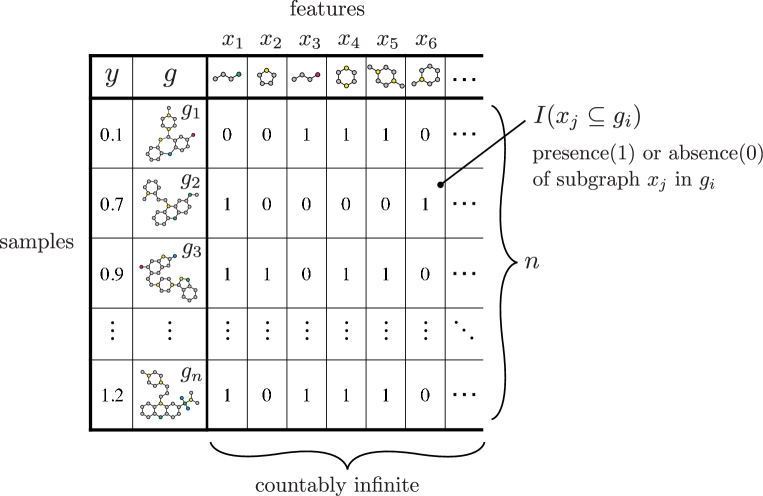
Figure 1: The design matrix for $g_{1},g_{2},\dots,g_{n}$ defined by subgraph indicators. This matrix can be obtained explicitly if the size of subgraph features is limited beforehand. In general, however, typical subgraph features are countably infinite, resulting in that we cannot obtain this matrix explicitly.

Our interest in Problem (1) is to statistically model the response $y$ to an input graph $g$ as $y=\mu(g)$ with a model function $\mu$. Whether explicitly or not, existing methods use subgraph indicators as explanatory variables. A subgraph indicator $I(x\subseteq g)\in\{0,1\}$ indicates the presence or absence of a subgraph feature $x\in\mathcal{G}$ in the input graph $g\in\mathcal{G}$.

Once if we fix explanatory variables to use, this problem takes a typical form of supervised-learning problems. We can then think of the sample-by-feature design matrix that is characterized by the set of all possible subgraph indicators. Figure 1 shows an example of the design matrix. However, we cannot explicitly obtain this matrix in practical situations. The number of possible subgraphs is countably infinite, and it is impossible in general to enumerate all possible subgraphs beforehand. Moreover, we need to test subgraph isomorphism to obtain each of $0$ or $1$ in the matrix. Only after we query a particular subgraph $x_{i}\in\mathcal{G}$ to a given set of $n$ graphs, $g_{1},g_{2},\dots,g_{n}$, we can obtain the corresponding column vector to $x_{i}$. At the beginning of the learning phase, we have no column vectors at all.

Hence the main difficulty of statistical learning problems from a set of graphs is simultaneous learning of the model function $\mu$ and a finite set of relevant features $\{x_{1},x_{2},x_{3},\dots\}\subset\mathcal{G}$. In practice we need to select some features among all possible subgraph features, but we do not know in advance subgraph features that are most relevant to a given problem. We thus need to search all possible subgraph features during the learning process.

In this paper, we consider a standard linear model over all possible subgraph indicators

$$\mu(g;\beta,\beta_{0}):=\beta_{0}+\sum_{j=1}^{\infty}\beta_{j}I(x_{j}\subseteq g),\quad\beta=(\beta_{1},\beta_{2},\dots),$$

where we assume the sparsity on coefficient parameters: Most coefficients $\beta_{1},\beta_{2},\dots$ are zero and a few of them, at least a finite number of them, are nonzero. We write $\mu(g;\beta,\beta_{0})$ simply as a function of $g$, $\mu(g)$, whenever there is no possibility of confusion.

1.2 Contributions of This Work

• Main Result: We present a generic algorithm that solves the following class of supervised-learning problems

  $$\min_{\beta,\beta_{0}}\sum_{i=1}^{n}L\bigl{(}y_{i},\mu(g_{i};\beta,\beta_{0})\bigr{)}+\lambda_{1}\|\beta\|_{1}+\frac{\lambda_{2}}{2}\|\beta\|_{2}^{2},$$ (2)

  where $L$ is a twice differentiable loss function and $\lambda_{1},\lambda_{2}\geqslant 0$. We here pose the elastic-net type regularizer: The third term of 2-norm $\|\beta\|_{2}^{2}$ encourages highly correlated features to be averaged, while the second term of 1-norm $\|\beta\|_{1}$, a sparsity-inducing regularizer, encourages a sparse solution in the coefficients of these averaged features. Subgraph features have a highly correlated nature, due to the inclusion relation that $x_{i}$ can be a subgraph of another feature $x_{j}$, and due to the tendency that structural similarity between $x_{i}$ and $x_{j}$ implies strong correlation between their indicators $I(x_{i}\subseteq g)$ and $I(x_{j}\subseteq g)$. Our framework targets a wider class of sparse learning problems than the preceding studies such as Adaboost (Kudo et al., 2005), LARS/LASSO (Tsuda, 2007), sparse partial-least-squares (PLS) regression (Saigo et al., 2008), sparse principal component analysis (PCA) (Saigo and Tsuda, 2008), and LPBoost (Saigo et al., 2009).

• The proposed algorithm directly optimizes the objective function by making Block Coordinate Gradient Descent (Tseng and Yun, 2009; Yun and Toh, 2011) feasible over all possible subgraph indicators. It updates multiple nonzero features at each iteration with simultaneous subgraph feature learning, while existing methods are iterative procedures to find the best single feature at each iteration that improves the current model most by a branch-and-bound technique. The proposed algorithm shows faster and more stable convergence.

• We formally generalize the underlying bounding techniques behind existing methods to what we call Morishita-Kudo Bounds by extending the technique used for Adaboost (Morishita, 2002; Kudo et al., 2005) to that for arbitrary separable objective functions. This bounding is not only one of the keys to develop the proposed algorithm, but also gives a coherent and unifying view to understand how the existing methods work. We see this in several examples where this bounding easily and consistently gives the pruning bounds of existing methods.

• We also present another important technique, which we call Depth-First Dictionary Passing. It allows to establish the efficient search-space pruning of our proposed algorithm. This technique is important, because unlike existing methods, search-space pruning by the Morishita-Kudo bounds is not enough to making block coordinate gradient descent feasible over infinite subgraph features.

• We studied the convergence behavior of our method and the difference from two major existing approaches (Kudo et al., 2005; Saigo et al., 2009) through numerical experiments. We used a typical example of 1-norm-penalized logistic regression estimated by the proposed algorithm. For systematic evaluations, we developed a random graph generator to generate a controllable set of graphs for binary classification. As a result, in addition to understanding the difference in the convergence behaviors, we pointed out and discussed several unnoticed issues including the size bias of subgraph features and the equivalence class of subgraph indicators.

1.3 Related Work

Under the setting of Figure 1, the most well-used machine learning approach for solving Problem (1) would be graph kernel method. So far various types of graph kernels have been developed and also achieved success in applications such as bioinformatics and chemoinformatics (Kashima et al., 2003; Gärtner et al., 2003; Ralaivola et al., 2005; Fröhlich et al., 2006; Mahé et al., 2005, 2006; Mahé and Vert, 2009; Kondor and Borgwardt, 2008; Kondor et al., 2009; Vishwanathan et al., 2010; Shervashidze et al., 2011). For example, we can compute the inner product of feature vectors of $g_{i}$ and $g_{j}$ in Figure 1, indirectly through a kernel trick as

$$k(g_{i},g_{j}):=\text{\# of common subgraphs between $g_{i}$ and $g_{j}$},$$

which is, as well as many other proper graph kernels, a special case of R-convolution kernels by Haussler (1999). However Gärtner et al. (2003) showed that (i) computing any complete graph kernel is at least as hard as deciding whether two graphs are isomorphic, and (ii) computing the inner product in the subgraph feature space is NP-hard. Hence, any practical graph kernel restricts the subgraph features to some limited types such as paths and trees, bounded-size subgraphs, or heuristically inspired subgraph features in application-specific situations.

In chemoinformatics, there have been many methods for computing the fingerprint descriptor (feature vector) of a given molecular graph. The predefined set of subgraph features engineered with the domain knowledge would be still often used, such as the existence of aromatic-ring or a particular type of functional groups. The success of this approach highly depends on whether the choice of features well fits the intrinsic property of data. To address this lack of generality, chemoinformatics community has developed data-driven fingerprints, for example, hashed fingerprints (such as Daylight and ChemAxon), extended connectivity fingerprints (ECFP) (Rogers and Hahn, 2010), frequent subgraphs (Deshpande et al., 2005), and bounded-size graph fingerprint (Wale et al., 2008). The data-driven fingerprints adaptively choose the subgraph features from a limited type of subgraphs, resulting in that these fingerprints are similar to practical graph kernels.

These two existing, popular approaches are based on subgraph features, which are limited to specific type ones only. In contrast, a series of inspiring studies for simultaneous feature learning via sparse modeling has been made (Kudo et al., 2005; Tsuda and Kudo, 2006; Tsuda, 2007; Tsuda and Kurihara, 2008; Saigo et al., 2008; Saigo and Tsuda, 2008; Saigo et al., 2009). These approaches involve automatic selection of relevant features from all possible subgraphs during the learning process. Triggered by the seminal paper by Kudo et al. (2005), it has been shown that we can perform simultaneous learning of not only the model parameters but also relevant subgraph features from all possible subgraphs in several machine-learning problems such as Adaboost (Kudo et al., 2005), LARS/LASSO (Tsuda, 2007), sparse partial-least-squares (PLS) regression (Saigo et al., 2008), sparse principal component analysis (PCA) (Saigo and Tsuda, 2008), and LPBoost (Saigo et al., 2009). This paper aims to give a coherent and unifying view to understand how these existing methods work well, and then present a more general framework, which is applicable to a wider class of learning problems.

2 Preliminaries

In this section, we formally define our problem and notations (Section 2.1), and summarize basic known results needed for the subsequent sections (Section 2.2).

2.1 Problem Formulation and Notations

First, we formulate our problem described briefly in Introduction. We follow the traditional setting of learning from graph data. Let $\mathcal{G}$ be a set of all finite-size, node-and-edge-labeled, connected, undirected graphs with finite discrete label sets for nodes and labels. We assume that data graphs $g_{1},g_{2},\dots,g_{n}$ and their subgraph features $x_{1},x_{2},\dots$ are all in $\mathcal{G}$. We write the given set of $n$ graphs as

$$\mathcal{G}_{n}:=\{g_{1},g_{2},\dots,g_{n}\},$$

and the label space as $\mathcal{Y}$, for example, $\mathcal{Y}=\mathbb{R}$ for regression and $\mathcal{Y}=\{T,F\}$ or $\{-1,1\}$ for binary classification.

Then we study the following problem where the 1-norm regularizer $\|\beta\|_{1}$ induces a sparse solution for $\beta$, i.e. a solution, in which only a few of $\beta_{1},\beta_{2},\dots$ are nonzero. The nonzero coefficients bring the effect of automatic selection of relevant features among all possible subgraphs.

Problem 1

For a given pair of observed graphs and their responses

$$\{(g_{1},y_{1}),(g_{2},y_{2}),\dots,(g_{n},y_{n})\},\quad g_{i}\in\mathcal{G},\quad y_{i}\in\mathcal{Y},$$

solve the following supervised-learning problem:

$$\min_{\beta,\beta_{0}}\sum_{i=1}^{n}L\bigl{(}y_{i},\mu(g_{i};\beta,\beta_{0})\bigr{)}+\lambda_{1}\|\beta\|_{1}+\frac{\lambda_{2}}{2}\|\beta\|_{2}^{2},$$ (3)

where $L$ is a twice-differentiable loss function, $\lambda_{1},\lambda_{2}\geqslant 0$, and the model function $\mu:\mathcal{G}\to\mathcal{Y}$ is defined as

$$\mu(g;\beta,\beta_{0}):=\beta_{0}+\sum_{j=1}^{\infty}\beta_{j}I(x_{j}\subseteq g),\quad\beta=(\beta_{1},\beta_{2},\dots),$$ (4)

where $x_{1},x_{2},\dots\in\mathcal{G}$.

Next, we define several notations that we use throughout the paper. $I(A)$ is a binary indicator function of an event $A$, meaning that $I(A)=1$ if $A$ is true; otherwise $I(A)=0$. The notation $x\subseteq g$ denotes the subgraph isomorphism that $g$ contains a subgraph that is isomorphic to $x$. Hence the subgraph indicator $I(x\subseteq g)=1$ if $x\subseteq g$; otherwise $0$.

Given $\mathcal{G}_{n}$, we define the union of all subgraphs of $g\in\mathcal{G}_{n}$ as

$$\mathcal{X}(\mathcal{G}_{n}):=\{x\in\mathcal{G}\mid x\subseteq g,g\in\mathcal{G}_{n}\}.$$

It is important to note that $\mathcal{X}(\mathcal{G}_{n})$ is a finite set and is equal to the set of subgraphs each of which is contained in at least one of the given graphs in $\mathcal{G}_{n}$ as

$$\mathcal{X}(\mathcal{G}_{n})=\{x\in\mathcal{G}\mid\text{$\exists g\in\mathcal{G}_{n}$ such that $x\subseteq g$}\}.$$

For given $\mathcal{X}(\mathcal{G}_{n})$, we can construct an enumeration tree over $\mathcal{X}(\mathcal{G}_{n})$ that is fully defined and explained in Section 2.2. Also we write a subtree of $\mathcal{T}(\mathcal{G}_{n})$ rooted at $x\in\mathcal{X}(\mathcal{G}_{n})$ as $\mathcal{T}(x)$ (See Figure 3).

For given $\mathcal{G}_{n}$ and a subgraph feature $x$, we define the observed indicator vector of $x$ over $\mathcal{G}_{n}$ as

$$I_{\mathcal{G}_{n}}(x):=(I(x\subseteq g_{1}),I(x\subseteq g_{2}),\dots,I(x\subseteq g_{n})).$$ (5)

From the definition, $I_{\mathcal{G}_{n}}(x)$ is an $n$-dimensional Boolean vector, that is, $I_{\mathcal{G}_{n}}(x)\in\{0,1\}^{n}$, which corresponds to each column vector of the design matrix in Figure 1.

For an $n$-dimensional Boolean vector $u:=(u_{1},u_{2},\dots,u_{n})\in\{0,1\}^{n}$, we write the index set of nonzero elements and that of zero elements as

$$1(u):=\{i\mid u_{i}=1\}\subseteq\{1,2,\dots,n\},\qquad 0(u):=\{i\mid u_{i}=0\}\subseteq\{1,2,\dots,n\}.$$

From the definition, we have $1(u)\cup 0(u)=\{1,2,\dots,n\}$ and $1(u)\cap 0(u)=\varnothing$. For simplicity, we also use the same notation for the observed indicator vector of $x$ as

$$1(x) :=1(I_{\mathcal{G}_{n}}(x))=\{i\mid x\subseteq g_{i},g_{i}\in\mathcal{G}_{n}\},$$

$$0(x) :=0(I_{\mathcal{G}_{n}}(x))=\{i\mid x\not\subseteq g_{i},g_{i}\in\mathcal{G}_{n}\}.$$

whenever there is no possibility of confusion.

2.2 Structuring the Search Space

Our target model of (4) includes an infinite number of terms that directly come from the infinite number of possible subgraph features $x_{1},x_{2},\dots$. We first briefly describe the algorithmic trick of reducing a set of countably infinite subgraph features to a well-structured finite search space which forms the common backbone of many preceding studies (Kudo et al., 2005; Tsuda, 2007; Saigo et al., 2008, 2009; Takigawa and Mamitsuka, 2011).

In Problem (3), we observe that the model function $\mu(g)$ appears only as the function values at given graphs, $\mu(g_{1}),\mu(g_{2}),\dots,\mu(g_{n})$. Correspondingly, the term $I(x_{j}\subseteq g)$ in the summation of the model (4) also only appears as the values at $\mathcal{G}_{n}$, that is, as $I(x_{j}\subseteq g_{1}),I(x_{j}\subseteq g_{2}),\dots,I(x_{j}\subseteq g_{n})$ for each $x_{j}$. Hence, as far as Problem (3) concerns, we can ignore all subgraphs $x^{\prime}$ that never occur in $g\in\mathcal{G}_{n}$ because $I(x^{\prime}\subseteq g_{i})=0$ for $i=1,2,\dots,n$ and they do not contribute to any final value of $\mu(g_{1}),\mu(g_{2}),\dots,\mu(g_{n})$. Therefore, for any $g\in\mathcal{G}_{n}$, we have

$$\mu(g;\beta,\beta_{0}):=\beta_{0}+\sum_{j=1}^{\infty}\beta_{j}I(x_{j}\subseteq g)=\beta_{0}+\sum_{x_{j}\in\mathcal{X}(\mathcal{G}_{n})}\beta_{j}I(x_{j}\subseteq g).$$

Furthermore, it will be noticed that $\mathcal{X}(\mathcal{G}_{n})$ equals to a set of frequent subgraphs in $\mathcal{G}_{n}$ whose frequency $\geqslant 1$, and the points so far can be summarized as follows.

Lemma 1

Without loss of generality, when we consider Problem (3), we can limit the search space of subgraphs $x_{j}$ to the finite set $\mathcal{X}(\mathcal{G}_{n})$ that is equivalent to a set of all frequent subgraphs in $\mathcal{G}_{n}$ with the minimum support threshold of one.

This fact connects Problem (3) to the problem of enumerating all frequent subgraphs in the given set of graphs—frequent subgraph pattern mining—that has been extensively studied in the data mining field. At this point, since $\mathcal{X}(\mathcal{G}_{n})$ is finite, we can say that Problem (3) with the linear model (4) is solvable in theory if we have infinite time and memory space. However, the set of $\mathcal{X}(\mathcal{G}_{n})$ is still intractably huge in general, and it is still practically impossible to enumerate all subgraphs in $\mathcal{X}(\mathcal{G}_{n})$ beforehand.

However the research on mining algorithms of frequent subgraph patterns brings a well-structured search space for $\mathcal{X}(\mathcal{G}_{n})$, called an enumeration tree, which has two nice properties, to be explained below. The enumeration tree can be generated from a so-called Hasse diagram, which is a rooted graph, each node being labeled by a subgraph, where parent-child relationships over labels correspond to isomorphic relationships and each layer has subgraphs with the same size. Figure 2 is schematic pictures of (a) a set of subgraphs, $\mathcal{X}(\mathcal{G}_{n})$, (b) a Hasse diagram over $\mathcal{X}(\mathcal{G}_{n})$, and (c) an enumeration tree over $\mathcal{X}(\mathcal{G}_{n})$.

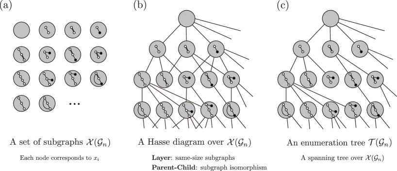
Figure 2: Non-redundant check of all elements in set $\mathcal{X}(\mathcal{G}_{n})$. (a) set $\mathcal{X}(\mathcal{G}_{n})$, (b) Hasse diagram for the set $\mathcal{X}(\mathcal{G}_{n})$, and (c) a tree-shaped search space, enumeration tree $\mathcal{T}(\mathcal{G}_{n})$ for the set $\mathcal{X}(\mathcal{G}_{n})$ which allows to search over a finite set of relevant subgraphs, $\mathcal{X}(\mathcal{G}_{n})$, without any redundancy.

1. Isomorphic parent-child relationship: Smaller subgraphs are assigned to the shallower levels, larger subgraphs to the deeper levels. The edge from $x_{i}$ to $x_{j}$ implies that $x_{i}$ and $x_{j}$ are different by only one edge, and $x_{i}$ at the shallower level is isomorphic to the subgraph of $x_{i}$ at the deeper level. This property is inherited from the Hasse diagram.

2. Spanning tree: Traversal over the entire enumeration tree gives us a set of all subgraphs $x_{j}$ in $\mathcal{X}(\mathcal{G}_{n})$, avoiding any redundancy in checking subgraphs, meaning that the same subgraph is not checked more than once.

For example, the gSpan algorithm, a well-established algorithm for frequent subgraph pattern mining, uses an enumeration tree by an algorithmic technique called right-most extension, where the enumeration tree is traversed in a depth-first manner (Yan and Han, 2002; Takigawa and Mamitsuka, 2011).

Our main interest is to efficiently search the subgraphs that should be checked, using enumeration tree $\mathcal{T}(\mathcal{G}_{n})$ to solve Problem (3) in terms of Model function (4). Throughout this paper, we use the enumeration tree by the gSpan algorithm as a search space for $\mathcal{X}(\mathcal{G}_{n})$.

The above fact can be formally summarized as follows.

Lemma 2

Let $G:=(V,E)$ be a graph with a node set $V=\mathcal{X}(\mathcal{G}_{n})\cap\{\varnothing\}$ and an edge set $E=\{(x,x^{\prime})\mid x\subseteq x^{\prime},x\in V,x^{\prime}\in V,\text{$x$ and $x^{\prime}$ are different by only one edge}\}$, where $\varnothing$ denotes the empty graph. Then, this graph $G$ corresponds to the Hasse diagram in Figure 2 (b). Moreover we can construct a spanning tree $\mathcal{T}(\mathcal{G}_{n})$ rooted at $\varnothing$ over $G$, that is, an enumeration tree for $\mathcal{X}(\mathcal{G}_{n})$ that has the following properties.

1. It covers all of $x\in\mathcal{X}(\mathcal{G}_{n})$, where any of $x\in\mathcal{X}(\mathcal{G}_{n})$ is reachable from the root $\varnothing$.

2. For a subtree $\mathcal{T}(x)$ rooted at node $x$, we have $x\subseteq x^{\prime}$ for any $x^{\prime}\in\mathcal{T}(x)$.

It is important to note that, from the second property in Lemma 2, we have

Lemma 3

$$I(x\subseteq g)=0\Longrightarrow I(x^{\prime}\subseteq g)=0,x^{\prime}\in\mathcal{T}(x).$$

In other words, once if we know $x\not\subseteq g$, then we can skip checking of all $x^{\prime}\in\mathcal{T}(x)$ because $x^{\prime}\not\subseteq g$. This fact serves as the foundation for many efficient algorithms of frequent subgraph pattern mining, including the gSpan algorithm.

3 Morishita-Kudo Bounds for Separable Functions

In this section, we formally generalize the underlying bounding technique, which was originally developed for using Adaboost (Morishita, 2002; Kudo et al., 2005) for subgraph features, to the one that we call Morishita-Kudo Bounds. Our generalization is an extension to that for arbitrary separable objective functions. This bounding is not only one of the keys to develop the proposed algorithm but also gives a coherent and unifying view to understand how the existing methods work. In Section 3.3, we show several examples, in which this bounding easily and consistently gives the pruning bounds of existing methods.

3.1 Bounding for Branch and Bound

Consider the problem of finding the best subgraph feature $x$ by using given training data $(y_{1},g_{1})$, $(y_{2},g_{2}),\dots,(y_{n},g_{n})$, when we predict the response $y$ by only one subgraph indicator $I(x\subseteq g)$. This subproblem constitutes the basis for the existing methods such as Adaboost (Kudo et al., 2005) and LPBoost (Saigo et al., 2009). The evaluation criteria can be various as follows, which characterize individual methods:

1. Maximizer of the weighted gain

   $$\textstyle\sum_{i=1}^{n}w_{i}y_{i}(2I(x\subseteq g_{i})-1)\,\,\text{for $y_{i}\in\{-1,1\}$}$$

2. Minimizer of the weighted classification error

   $$\textstyle\sum_{i=1}^{n}w_{i}I(I(x\subseteq g_{i})\neq y_{i})\,\,\text{for $y_{i}\in\{0,1\}$}$$

3. Maximizer of the correlation to the response

   $$\textstyle{\Big{|}}\sum_{i=1}^{n}y_{i}I(x\subseteq g_{i}){\Big{|}}\,\,\text{for $y_{i}\in\mathbb{R}$}$$

It should be noted that there exist multiple optimal subgraphs, and any one of such subgraphs can be the best subgraph feature.

All of these problems take a form of finding the single subgraph $x^{*}$ that minimizes or maximizes some function $f(x)$ dependent on the given graphs $\mathcal{G}_{n}$. A brute-force way to obtain the best solution $x^{*}=\arg\min_{x}f(x)$ would be to first traverse all $x_{j}$ in the enumeration tree $\mathcal{T}(\mathcal{G}_{n})$, compute the value of $f(x_{j})$ at each node $x_{j}$, and then take the best one among $\{f(x_{j})\mid x_{j}\in\mathcal{T}(\mathcal{G}_{n})\}$ after all $x_{j}$ are checked. Unfortunately this brute-force enumeration does not work in reality because the size of the set $\mathcal{X}(\mathcal{G}_{n})$ is intractably large in most practical situations.

In existing work, this problem has been addressed by using branch and bound. Due to the nice property of an enumeration tree shown in Lemma 2 and 3, we can often know the upper and lower bounds of $f(x^{\prime})$ for any subgraph $x^{\prime}$ in the subtree below $x$, i.e. $x^{\prime}\in\mathcal{T}(x)$, without checking the values of every $f(x^{\prime})$. In other words, when we are at node $x$ of an enumeration tree during traversal over the tree, we can obtain two values $\overline{c}(x)$ and $\underline{c}(x)$ dependent on $x$ that shows

$$\underline{c}(x)\leqslant f(x^{\prime})\leqslant\overline{c}(x)\,\,\text{for any $x^{\prime}\in\mathcal{T}(x)$}$$

without actually checking $f(x^{\prime})$ for $x^{\prime}\in\mathcal{T}(x)$.

Then, if the tentative best solution $\hat{x}$ among already visited nodes before the current $x$ is better than the best possible value in the subtree $\mathcal{T}(x)$, i.e. $f(\hat{x})<\underline{c}(x)$ (for finding the minimum $x^{*}$) or $f(\hat{x})>\overline{c}(x)$ (for finding the maximum $x^{*}$), we can prune the subtree $\mathcal{T}(x)$ and skip all checking of unseen subgraphs $x^{\prime}\in\mathcal{T}(x)$.

In order to perform this branch and bound strategy, we need a systematic way to get the upper and lower bounds for a given objective function. In existing work, these bounds have been derived separately for each specific objective function such as Adaboost (Kudo et al., 2005), LPBoost (Saigo et al., 2009), LARS/LASSO (Tsuda, 2007) and PLS regression (Saigo et al., 2008). In the following subsections, we show that we can generalize the common technique behind these existing approaches to what we call Morishita-Kudo Bounds, which was developed for the preceding studies based on Adaboost (Morishita, 2002; Kudo et al., 2005).

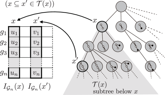
Figure 3: Boolean vectors $I_{\mathcal{G}_{n}}(x)$ associated with $x\in\mathcal{T}(\mathcal{G}_{n})$. In this example, $x\subseteq x^{\prime}$. Hence $v_{i}=0$ for $u_{i}=0$. Only coordinates $v_{i}$ for $u_{i}=1$ can be either $0$ or $1$, as stated in Lemma 4.

3.2 Property of Boolean Vectors Associated with $\mathcal{G}_{n}$

First, we observe that the following result holds from Lemma 2 and 3.

Lemma 4

$1(I_{\mathcal{G}_{n}}(x^{\prime}))\subseteq 1(I_{\mathcal{G}_{n}}(x))$ for $x^{\prime}\in\mathcal{T}(x)$. For short, $1(x^{\prime})\subseteq 1(x)$ for $x^{\prime}\in\mathcal{T}(x)$.

Remark 5

Recall that $I_{\mathcal{G}_{n}}(x)$, previously defined as (5), is the observed indicator vector, an $n$-dimensional Boolean vector, indicating if $x$ is contained in each of $\mathcal{G}_{n}$. The number of $1$s in the vector $I_{\mathcal{G}_{n}}(x)$, that is $|1(I_{\mathcal{G}_{n}}(x))|$, is identical to the “support” of $x$ in $\mathcal{G}_{n}$ in the standard data mining terminology.

Lemma 4, as well as Lemma 3, claims that when we traverse an enumeration tree down to the deeper level from $x$ to $x^{\prime}$, the elements taking $1$ in $I_{\mathcal{G}_{n}}(x)$ can change to $1$ or $0$ but the elements taking $0$ must remain as $0$ in $I_{\mathcal{G}_{n}}(x^{\prime})$. Figure 3 schematically shows this property of enumeration trees. More explicitly, let $I_{\mathcal{G}_{n}}(x)=(u_{1},u_{2},\dots,u_{n})$ and $I_{\mathcal{G}_{n}}(x^{\prime})=(v_{1},v_{2},\dots,v_{n})$. Then,

$$v_{i}=\begin{cases}0&\text{$(u_{i}=0)$}\\ \text{$0$ or $1$}&\text{$(u_{i}=1)$}.\end{cases}$$

This fact also implies that the number of $1$s in the associated Boolean vector $I_{\mathcal{G}_{n}}(x)$ at node $x$ monotonically decreases if we proceed to any deeper node $x^{\prime}(\supseteq x)$ in the enumeration tree. The anti-monotone property of the support, which is a fundamental technique in frequent pattern mining, can also be obtained as a corollary of Lemma 4 as

$$x\subseteq x^{\prime}\Longrightarrow|1(I_{\mathcal{G}_{n}}(x))|\geqslant|1(I_{\mathcal{G}_{n}}(x^{\prime}))|.$$

We also observe the following simple facts for arbitrary bounded real-valued function on $n$-dimensional Boolean vector space, $f:\{0,1\}^{n}\to\mathbb{R}$.

Theorem 6

Assume that $u=(u_{1},u_{2},\dots,u_{n})\in\{0,1\}^{n}$ are given. Then, for any $v=(v_{1},v_{2},\dots,v_{n})\in\{0,1\}^{n}$ such that $1(v)\subseteq 1(u)$, we have

$$\overline{f}(u)\geqslant f(v)\geqslant\underline{f}(u),$$

where

$$\overline{f}(u) =\max_{\alpha_{i}\in\{0,1\},i\in 1(u)}\{f(\alpha_{1},\alpha_{2},\dots,\alpha_{n})\mid\alpha_{j}=0,j\in 0(u)\},$$

$$\underline{f}(u) =\min_{\alpha_{i}\in\{0,1\},i\in 1(u)}\{f(\alpha_{1},\alpha_{2},\dots,\alpha_{n})\mid\alpha_{j}=0,j\in 0(u)\}.$$

These $\overline{f}(u)$ and $\underline{f}(u)$ are non-trivial bounds of $f(v)$ when they respectively satisfy

$$\overline{f}(u)<\max_{w\in\{0,1\}^{n}}f(w)\quad\text{and}\quad\underline{f}(u)>\min_{w\in\{0,1\}^{n}}f(w).$$

Proof  Since $1(v)\subseteq 1(u)\Leftrightarrow 0(u)\subseteq 0(v)$, we have $u_{i}=0\Rightarrow v_{i}=0$ for any $v$ such that $1(v)\subseteq 1(u)$. Thus, fixing all $i\in 0(u)$ as $v_{i}=0$ and setting the remaining $v_{i},i\in 1(u)$ free as

$$\{f(v)\mid 1(v)\subseteq 1(u)\}=\{f(\alpha_{1},\alpha_{2},\dots,\alpha_{n})\mid\alpha_{i}=0,i\in 0(u)\},$$

and taking the maximum and minimum in this set leads to the result in the theorem. Note that the above set is finite since $\alpha_{i}\in\{0,1\},i\in 1(u)$.  

Corollary 7

From Theorem 6, we can have the upper and lower bounds of $f(I_{\mathcal{G}_{n}}(x^{\prime}))$ at any $x^{\prime}\in\mathcal{T}(x)$ for any function $f:\{0,1\}^{n}\to\mathbb{R}$ as

$$\overline{f}(I_{\mathcal{G}_{n}}(x))\geqslant f(I_{\mathcal{G}_{n}}(x^{\prime}))\geqslant\underline{f}(I_{\mathcal{G}_{n}}(x)),$$

because $1(I_{\mathcal{G}_{n}}(x^{\prime}))\subseteq 1(I_{\mathcal{G}_{n}}(x))$ for $x^{\prime}\in\mathcal{T}(x)$ from Lemma 4.

3.3 Morishita-Kudo Bounds and Their Examples

Theorem 6 and Corollary 7 give us a general idea to obtain pruning bounds for arbitrary function $f$ in the depth-first traversal of an enumeration tree. Furthermore, applying Theorem 6 to separable functions enables us to obtain the following easy-to-compute bounds that we call Morishita-Kudo bounds. Note that the target functions appeared in the existing studies such as Morishita (2002); Kudo et al. (2005); Tsuda (2007); Saigo et al. (2008, 2009) are all separable functions.

Lemma 8 (Morishita-Kudo bounds)

Assume that a real-valued function of $n$-dimensional Boolean vector $f:\{0,1\}^{n}\to\mathbb{R}$ is separable, meaning that there exists a set of $n$ functions $f_{i}:\{0,1\}\to\mathbb{R},i=1,2,\dots,n$ and

$$f(u_{1},u_{2},\dots,u_{n})=\sum_{i=1}^{n}f_{i}(u_{i}),\quad u_{i}\in\{0,1\}.$$

Then, for given $u=(u_{1},u_{2},\dots,u_{n})\in\{0,1\}^{n}$, we have

$$\overline{f}(u)\geqslant f(v)\geqslant\underline{f}(u)$$

for any $v=(v_{1},v_{2},\dots,v_{n})\in\{0,1\}^{n}$ such that $1(v)\subseteq 1(u)$, where

$$\underline{f}(u) :=\sum_{i\in 1(u)}\min\{f_{i}(0),f_{i}(1)\}\,\,+\sum_{i\in 0(u)}f_{i}(0)$$

$$\overline{f}(u) :=\sum_{i\in 1(u)}\max\{f_{i}(0),f_{i}(1)\}\,\,+\sum_{i\in 0(u)}f_{i}(0)$$

Thus, for separable functions, if we have some fixed $u\in\{0,1\}^{n}$, then we can limit the possible range of $f(v)$ for any $v$ such that $1(v)\subseteq 1(u)$, and the upper and lower bounds for $f(v)$, i.e. $\underline{f}(u)$ and $\overline{f}(u)$, are easy to compute just by comparing $f_{i}(0)$ and $f_{i}(1)$ for each $i\in 1(u)$. Since $1(v)\subseteq 1(u)$, we have $v_{i}=0$ for $i\in 0(u)$ and the amount of $\sum_{i\in 0(u)}f_{i}(0)$ is unchanged and cannot be further improved. Only elements that can differ are $v_{i}$s for $i\in 1(u)$, and therefore we have the maximum or minimum of $f(v)$ for $v$ such that $1(v)\subseteq 1(u)$.

The original bounds by Morishita (2002); Kudo et al. (2005) target only the specific objective function of Adaboost, but many existing methods for other objectives, such as Tsuda (2007); Saigo et al. (2008, 2009), which share the common idea as described in Lemma 8. Indeed most existing approaches are based on a branch-and-bound strategy with the Morishita-Kudo bounds for each class of learning problems with separable loss functions. We see this fact in the three examples below.

3.3.1 Example 1: Find a subgraph that maximizes the gain

Assume that we have a certain subgraph $x$ at hand. For the problem of classification with $y_{i}\in\{-1,1\}$, consider the upper bound of the gain attained by subgraph $z$ ($\supseteq x$)

$$\sum_{i=1}^{n}w_{i}y_{i}(2I(z\subseteq g_{i})-1)$$

by $-1/1$-valued features of $2I(z\subseteq g_{i})-1$, where $w_{i}\geqslant 0$ (Kudo et al., 2005). Then, from Lemma 4, we have $x\subseteq z\Rightarrow 1(z)\subseteq 1(x)$. Thus we obtain a Morishita-Kudo upper bound

$$\sum_{i=1}^{n}w_{i}y_{i}(2I(z\subseteq g_{i})-1) \leqslant\sum_{i\in 1(x)}\max\{w_{i}y_{i}(2\cdot 0-1),w_{i}y_{i}(2\cdot 1-1)\}+\sum_{i\in 0(x)}w_{i}y_{i}(2\cdot 0-1)$$

$$=\sum_{i\in 1(x)}\max\{-w_{i}y_{i},w_{i}y_{i}\}-\sum_{i\in 0(x)}w_{i}y_{i}=\sum_{i\in 1(x)}w_{i}-\sum_{i\in 0(x)}w_{i}y_{i}.$$

In the original paper of Kudo et al. (2005), this bound was derived as

$$\sum_{i=1}^{n}w_{i}y_{i}(2I(z\subseteq g_{i})-1) =2\sum_{i=1}^{n}w_{i}y_{i}I(z\subseteq g_{i})-\sum_{i=1}^{n}w_{i}y_{i}$$

$$\leqslant 2\left\{\sum_{i\in 1(x)}\max\{w_{i}y_{i},0\}+\sum_{i\in 0(x)}w_{i}y_{i}\cdot 0\right\}-\sum_{i=1}^{n}w_{i}y_{i}$$

$$=2\sum_{i\in 1(x)\wedge y_{i}=1}w_{i}-\sum_{i=1}^{n}w_{i}y_{i}.$$

We can confirm that these two are equivalent as $\sum_{i\in 1(x)}w_{i}-\sum_{i\in 0(x)}w_{i}y_{i}=2\sum_{i\in 1(x)\wedge y_{i}=1}w_{i}-\sum_{i=1}^{n}w_{i}y_{i}$ by subtracting the right-hand side from the left-hand side.

3.3.2 Example 2: Find a subgraph that minimizes the classification error

Assume that we have a certain subgraph $x$ at hand. For the problem of classification with $y_{i}\in\{0,1\}$, consider the lower bound of the weighted classification error attained by $z$ ($\supseteq x$)

$$\sum_{i=1}^{n}w_{i}I(I(z\subseteq g_{i})\neq y_{i}),$$

where $w_{i}\geqslant 0$. Similarly we have a Morishita-Kudo lower bound

$$\sum_{i=1}^{n}w_{i}I(I(z\subseteq g_{i})\neq y_{i}) \geqslant\sum_{i\in 1(x)}\min\{w_{i}I(0\neq y_{i}),w_{i}I(1\neq y_{i})\}+\sum_{i\in 0(x)}w_{i}I(0\neq y_{i})$$

$$=\sum_{i\in 0(x)}w_{i}I(0\neq y_{i})=\sum_{i\in 0(x)\wedge y_{i}=1}w_{i}.$$

In other words, the classification error depends only on elements taking $y_{i}=1$ but predicted as $I(x\subseteq g_{i})=0$. Once the predictor value becomes $0$, the objective function cannot be further improved by searching $z$ such that $z\supseteq x$. We can conclude that for $x$ such that the amount $\sum_{i\in 0(x)\wedge y_{i}=1}w_{i}$ is large, the possible value with $z$ by further searching $z$ such that $z\supseteq x$ is upper bounded by this amount.

3.3.3 Example 3: Find a subgraph that maximizes the correlation

Assume we have a certain subgraph $x$ at hand. As seen in regression problems (Saigo et al., 2009), consider the upper bound of the correlation between response $w_{i}\in\mathbb{R}$ and indicator $I(z\subseteq g_{i})$ by subgraph feature $z$ ($\supseteq x$)

$$\left|\sum_{i=1}^{n}w_{i}I(z\subseteq g_{i})\right|.$$

From $|a|=\max\{a,-a\}$, the larger amount of

$$\sum_{i=1}^{n}w_{i}I(z\subseteq g_{i})\qquad\text{or}\qquad-\sum_{i=1}^{n}w_{i}I(z\subseteq g_{i})$$

gives the upper bound of the correlation. Here we have a Morishita-Kudo upper bound as

$$\sum_{i=1}^{n}w_{i}I(z\subseteq g_{i})\leqslant\sum_{i\in 1(x)}\max\{w_{i}\cdot 0,w_{i}\cdot 1\}+\sum_{i\in 0(x)}w_{i}\cdot 0=\sum_{i\in 1(x)}\max\{0,w_{i}\}=\sum_{i\in 1(x)\wedge w_{i}>0}w_{i}.$$

We can always have $w_{i}I(x\subseteq g_{i})=0$ for $i\in 0(x)$, and rewrite as

$$\sum_{i=1}^{n}w_{i}I(z\subseteq g_{i})\leqslant\sum_{i\in 1(x)\wedge w_{i}>0}w_{i}=\sum_{w_{i}>0}w_{i}I(x\subseteq g_{i}).$$

Therefore, we can easily have the pruning bound in Saigo et al. (2009) as

$$\left|\sum_{i=1}^{n}w_{i}I(z\subseteq g_{i})\right|\leqslant\max\left\{\sum_{w_{i}>0}w_{i}I(x\subseteq g_{i}),-\sum_{w_{i}<0}w_{i}I(x\subseteq g_{i})\right\}.$$

4 Learning Sparse Liner Models by Block Coordinate Gradient Descent

Now we are back to our original problem, shown as Problem 1. In this section, we describe the optimization process for Problem 1, and in order to focus on this purpose, we first rewrite the problem in terms of parameters to be estimated, $\theta:=(\beta_{0},\beta)$, as nonsmooth optimization with a smooth part $f(\theta)$ and a nonsmooth part $R(\theta)$ as follows.

Problem 2

Find the minimizer

$$\theta^{*}=\arg\min_{\theta}F(\theta),\theta:=(\beta_{0},\beta),$$

where $F(\theta):=f(\theta)+R(\theta),\theta_{0}=\beta_{0},\theta_{1}=\beta_{1},\theta_{2}=\beta_{2},\dots$, and

$$f(\theta) :=\sum_{i=1}^{n}L\bigl{(}y_{i},\mu(g_{i};\beta,\beta_{0})\bigr{)}+\frac{\lambda_{2}}{2}\|\beta\|_{2}^{2}$$

$$R(\theta) :=\lambda_{1}\|\beta\|_{1}$$

Our basic premise behind Problem 2 is that we need a sparse solution for $\beta$, meaning that only a few of the coordinates $\beta_{1},\beta_{2},\dots$ are nonzero. Furthermore, whenever we have intermediate solutions for searching the optimal $\theta^{*}$, we also need to keep them sparse throughout the entire optimization process. This is simply because we have an intractably large number of parameters as $\beta_{1},\beta_{2},\dots$ even though Lemma 1 and 2 suggest that they are finite.

In addition, these parameters $\beta_{1},\beta_{2},\dots$ are associated with the corresponding subgraph features $x_{1},x_{2},\dots$ that also need to be estimated. In other words, in order to solve Problem 2, we need to perform simultaneous learning of the model coefficient $\beta_{i}$ and corresponding subgraph feature $x_{i}$, which are correspondingly paired as

$$\begin{array}[]{c}\beta_{1}\\ \updownarrow\\ x_{1}\end{array}\begin{array}[]{c}\beta_{2}\\ \updownarrow\\ x_{2}\end{array}\dots\begin{array}[]{c}\beta_{i}\\ \updownarrow\\ x_{i}\end{array}\dots\begin{array}[]{c}\beta_{m}\\ \updownarrow\\ x_{m}\end{array}$$

where $m=|\mathcal{X}(\mathcal{G}_{n})|$. Unlike standard situations in optimization, this problem has two remarkably challenging difficulties:

• We cannot estimate $\beta_{i}$ without finding the corresponding subgraph $x_{i}$. At the same time, however, it is practically impossible to find all subgraphs $x_{1},x_{2},\dots,x_{m}$ in advance.

• The number of parameters $m$ is unknown in advance and even not computable in most practical cases (intractably large) because of combinatorial explosion.

On the other hand, we notice that we do not need to check subgraph $x_{i}$ if we know $\beta_{i}=0$ beforehand.

Thus our idea for these two points is to start an iterative optimization process with all zero initial values as $\beta_{i}=0,i=1,2,\dots,m$, and search and trace subgraph features $x_{i}$ with nonzero $\beta_{i}$ after each iteration, avoiding the check for $x_{j}$ with $\beta_{j}=0$ as much as possible. Moreover, when we first start with the zero vector, i.e. $\theta(0)=0$, and then improve $\theta$ step by step as

$$\theta(0)\to\theta(1)\to\theta(2)\to\dots\to\theta^{*},$$

we kept all $\theta(t)$ sparse, meaning that only a few coordinates of every $\theta(t)$ are nonzero. More precisely, we need to meet the following two requirements.

1. First, we need an iterative optimization procedure with keeping all intermediate $\theta(t)$ sparse such that

   $$F(\theta(t))>F(\theta(t+1))\quad t=0,1,2,\dots$$

   that implies convergence for any lower bounded function $F$ from the monotone convergence theorem. Furthermore we also need to make sure that the solution converges to the optimal solution $\theta^{*}$ as $\lim_{t\to\infty}F(\theta(t))=F(\theta^{*})$.

2. Second, unlike standard cases, we need to perform the optimization with only the nonzero part of $\beta$ without even seeing the zero part of $\beta$ explicitly. In addition, we need to identify the nonzero part of $\theta$ at each step without checking subgraph $x_{i}$ that corresponds to $\beta_{i}=0$ as much as possible.

We present our approach for solving these two issues, the first and second points being in Section 4.1 and in Section 4.2, respectively.

4.1 Tseng-Yun Class of Block Coordinate Gradient Descent

Suppose hypothetically that our features are explicitly given beforehand as in the standard machine-learning situations. Then, there are many optimization procedures available for the nonsmooth objective functions in Problem 2 such as Proximal Gradient Method (Fukushima and Mine, 1981), Iterative Shrinkage/Thresholding (Figueiredo and Nowak, 2003; Daubechies et al., 2004), Operator Splitting (Combettes and Wajs, 2005), Fixed Point Continuation (Hale et al., 2008a, b), FISTA (Beck and Teboulle, 2009), SpaRSA (Wright et al., 2009), and glmnet (Friedman et al., 2007, 2010). Most of these methods are based on coordinate descent for efficiently finding the optimal sparse solution.

However, our problem is defined by the implicitly-given subgraph-indicator features, and we need to simultaneously learn the necessary subgraphs. To make things worse, since our problem has an intractably large number of parameters, we cannot even access to all parameter values. Therefore, it is impossible to simply apply these algorithms to our setting. Moreover, we need to keep all intermediate solutions sparse as well. Any generic solver based on interior-point methods, which can generate non-sparse intermediate solutions, also does not fit to our setting.

We thus extend a framework of block coordinate descent with small nonzero coordinate blocks to our simultaneous learning of features and parameters. Tseng and Yun (2009); Yun and Toh (2011) studied a class of block coordinate gradient descent for nonsmooth optimization appeared in Problem 2. They presented a fast algorithm and also established the global and linear convergence under a local error bound condition, as well as Q-linear convergence for 1-norm regularized convex minimization. Moreover, when we choose the coordinate block by a Gauss-Southwell-type rule, we can make all the intermediate solutions sparse without breaking the theoretical convergence property as we see below.

Their algorithm is based on gradient descent by applying local second-order approximation at the current $\theta(t)$ to only the smooth part $f(\theta)$ of the objective function $F(\theta)=f(\theta)+R(\theta)$ as

$$\min_{\theta}\left[f(\theta)+R(\theta)\right] =\min_{\theta}\left[f(\theta)-f(\theta(t))+R(\theta)\right]$$

$$\approx\min_{\theta}\left[\langle\nabla f(\theta(t)),\theta-\theta(t)\rangle+\frac{1}{2}\langle\theta-\theta(t),H(t)(\theta-\theta(t))\rangle+R(\theta)\right]$$

where $H(t)\succ 0$ is a positive-definite matrix approximating the Hessian $\nabla^{2}f(\theta(t))$. The main idea is to solve this local minimization by block coordinate descent instead of directly optimizing the original objective function by coordinate descent, which may be viewed as a hybrid of gradient projection and coordinate descent. The coordinate block to be updated at each iteration are chosen in a Gauss-Southwell way, which can be the entire coordinates or a small block of coordinates satisfying a required condition.

The algorithm first computes a descent direction $d(t):=T(\theta(t))-\theta(t)$ where

$$T(\theta(t)):=\arg\min_{\theta}\left[\langle\nabla f(\theta(t)),\theta-\theta(t)\rangle+\frac{1}{2}\langle\theta-\theta(t),H(t)(\theta-\theta(t))\rangle+R(\theta)\right]$$ (6)

which is optimized by block coordinate descent with a Gauss-Southwell type rule of coordinate block for $d(t)$. We choose the coordinate block by setting $d(t)_{j}=0$ for $j$ such that $v(t)\|d(t)\|_{\infty}>|d(t)_{j}|$ with some predefined scaling factor $v(t)$, which can adjust the sparsity of intermediate solutions. This coordinate block satisfies the Gauss-Southwell-r rule defined in Tseng and Yun (2009), which ensures the sufficient descent and global convergence. Next, the algorithm performs one-dimensional minimization of stepsize $\alpha(t)$ for the update of

$$\theta(t+1)\leftarrow\theta(t)+\alpha(t)\,d(t),\quad$$

by a line search with the following Armijo rule: choose $\alpha_{\mathrm{init}}(t)>0$ and let $\alpha(t)$ be the largest element of $\{\alpha_{\mathrm{init}}(t)\,s^{j}\},j=0,1,\dots$, where $s$ is a scaling parameter such that $0<s<1$, satisfying

$$F(\theta(t)+\alpha(t)d(t))\leqslant F(\theta(t))+\alpha(t)\sigma\Delta(t)$$ (7)

where $0<\sigma<1,0<\gamma<1$, and

$$\Delta(t):=\langle\nabla f(\theta(t)),d(t)\rangle+\gamma\langle d(t),H(t)d(t)\rangle+R(\theta(t)+d(t))-R(\theta(t)).$$

Note that since $\Delta(t)\leqslant(\gamma-1)\langle d(t),H(t)d(t)\rangle<0$, this rule guarantees that $F(\theta(t+1))<F(\theta(t))$ after the update of $\theta(t+1)\leftarrow\theta(t)+\alpha(t)d(t)$. The amount of $\alpha(t)\sigma\Delta(t)$ is required for guaranteeing not only the convergence to some point but also the convergence to the optimal solution (See their original papers for theoretical details). This Armijo rule is based on the following lemma (Lemma 1 in Tseng and Yun (2009)).

Lemma 9 (Tseng and Yun, 2009)

For any $\theta$ and $H\succ 0$, let $g=\nabla f(\theta)$ and $d_{J}=T(\theta)-\theta$ such that $d_{j}=0$ for $j$ in the index subset $J$. Then

$$F(\theta+\alpha d_{J})\leqslant F(\theta)+\alpha\left(\langle g,d_{J}\rangle+R(\theta+d_{J})-R(\theta)\right)+o(\alpha)\quad\forall\alpha\in(0,1]$$

$$\langle g,d_{J}\rangle+R(\theta+d_{J})-R(\theta)\leqslant-\langle d_{J},Hd_{J}\rangle.$$

4.2 Tracing Nonzero Coefficient Block of Subgraph Indicators

Now we consider how we can use the Tseng-Yun block coordinate gradient descent in our subgraph-search-required situations of Problem 1 (or equivalently Problem 2). Remember that the parameter space is intractably large due to the size of the accompanying subgraph space $\mathcal{X}(\mathcal{G}_{n})$. Each $j$-th coordinate of $\theta(t)$ is associated with the corresponding subgraph feature $x_{j}\in\mathcal{X}(\mathcal{G}_{n})$. Thus, we cannot even have $\theta(t)$ explicitly, and we need to perform the optimization process with tracing only the nonzero part of $\theta(t)$ without even seeing the zero part explicitly. Since we start with setting all coordinates of initial $\theta(0)$ to zero, it is enough to consider the update rule to compute $\theta(t+1)$ from the current $\theta(t)$ at hand. More precisely, we need a procedure to obtain the nonzero part of $\theta(t+1)$ from the nonzero part of $\theta(t)$ at hand.

Suppose that we have all nonzero coordinates of $\theta(t)$. The Tseng-Yun’s iterative procedure requires the following computations at each step of $\theta(t)\to\theta(t+1)$ until convergence:

1. Step 1. Compute $T(\theta(t))$ by coordinate descent for (6).

2. Step 2. Compute a descent direction by $d(t)=T(\theta(t))-\theta(t)$.

3. Step 3. Set Gauss-Southwell-r block by $d(t)_{j}=0$ for $\{j\mid v(t)\|d(t)\|_{\infty}>|d(t)_{j}|\}$.

4. Step 4. Do a line search for $\alpha(t)$ with the modified Armijo rule of (7).

5. Step 5. Update the parameter by $\theta(t+1)\leftarrow\theta(t)+\alpha(t)d(t)$.

Since we already have all nonzero coordinates of $\theta(t)$, the determining step to detect the nonzero part of $\theta(t+1)$ is Step 1. Indeed, if we obtain the nonzero part of $T(\theta(t))$, Step 2 to 5 follow just as in familiar optimization situations (See Figure 4 for a schematic example).

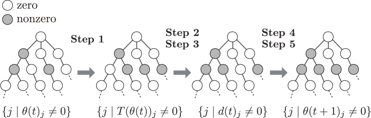
Figure 4: A schematic example of corresponding nonzero coordinates of $\theta(t)$, $T(\theta(t))$, $d(t)$, and $\theta(t+1)$ in the enumeration tree. The nonzero coordinates of $\theta(t+1)$ is computed from those of $\theta(t)$ through $T(\theta(t))$ and $d(t)$, and identifying $T(\theta(t))_{j}\neq 0$ is the determining step. Since $d(t)=T(\theta(t))-\theta(t)$, we have $\{j\mid d(t)_{j}\neq 0\}\subseteq\{j\mid\theta(t)_{j}\neq 0\}\cup\{j\mid T(\theta(t))_{j}\neq 0\}$. Since $\theta(t+1)=\theta(t)+\alpha(t)d(t)$, we can also see $\{j\mid\theta(t+1)_{j}\neq 0\}\subseteq\{j\mid\theta(t)_{j}\neq 0\}\cup\{j\mid T(\theta(t))_{j}\neq 0\}$.

We thus focus on how to identify the nonzero indices $\{j\mid T(\theta(t))_{j}\neq 0\}$ from the current $\theta(t)$ at hand (Step 1). Note that Step 1 is based on coordinate descent and the computation of each $i$-th coordinate $T(\theta(t))_{j}$ can be separately estimated. Also note that Step 3, 4 and 5 can be carried out only after Step 1 and 2 for all nonzero coordinates are obtained because Step 3 requires $\|d(t)\|_{\infty}$.

The starting point to realize Step 1 in our “graph” situations is the following lemma, which shows that $T(\theta(t))_{j}$ for the $j$-th coordinate has the closed-form solution.

Lemma 10

In Problem 1, when we solve (6) by coordinate descent, the following closed-form solution exists for each $j=1,2,\dots$:

$$T(\theta(t))_{j}=\begin{cases}-H(t)_{jj}^{-1}(b_{j}(t)+\lambda_{1})&b_{j}(t)<-\lambda_{1}\\ -H(t)_{jj}^{-1}(b_{j}(t)-\lambda_{1})&b_{j}(t)>\lambda_{1}\\ 0&|b_{j}(t)|\leqslant\lambda_{1}\end{cases}$$

where

$$b_{j}:=\sum_{i=1}^{n}\frac{\partial L(y_{i},\mu(g_{i};\theta(t)))}{\partial\theta(t)_{j}}+(\lambda_{2}-H(t)_{jj})\theta(t)_{j}.$$

Proof  See Appendix A1.  

Combined with the structured search space of $\mathcal{X}(\mathcal{G}_{n})$ which is equal to the enumeration tree $\mathcal{T}(\mathcal{G}_{n})$, Lemma 10 provides a way to examine if $T(\theta(t))_{k}=0$ for unseen $k$ such that $x_{k}\in\mathcal{T}(x_{j})$: When we know $T(\theta(t))_{k}=0$ for all unseen $x_{k}\in\mathcal{T}(x_{j})$, we can skip the check of all subgraphs in the subtree below $x_{j}$, i.e. $x_{k}\in\mathcal{T}(x_{j})$

As the lemma claims, $T(\theta(t))_{k}=0$ is controlled by whether $|b_{k}(t)|\leqslant\lambda_{1}$ or not. If we know the largest possible value $b_{j}^{*}$ of $|b_{k}(t)|$ for any $k$ such that $x_{k}\in\mathcal{T}(x_{j})$ and also know that $b_{j}^{*}\leqslant\lambda_{1}$, then we can conclude $T(\theta(t))_{k}=0$ for all of such $k$s. To consider how to obtain this bound $b_{j}^{*}$, let $b_{k}^{(1)}(t)$ and $b_{k}^{(2)}(t)$ be the first and second terms of $b_{k}(t)$, respectively, as

$$b_{k}^{(1)}(t):=\sum_{i=1}^{n}\frac{\partial L(y_{i},\mu(g_{i};\theta(t)))}{\partial\theta(t)_{k}},\qquad b_{k}^{(2)}(t):=(\lambda_{2}-H(t)_{kk})\theta(t)_{k}.$$

Then, since

$$\text{$|b^{(1)}+b^{(2)}|\leqslant\max\{\overline{b}^{(1)}+\overline{b}^{(2)},-\underline{b}^{(1)}-\underline{b}^{(2)}\}$ for any $\underline{b}^{(1)}\leqslant b^{(1)}\leqslant\overline{b}^{(1)},\underline{b}^{(2)}\leqslant b^{(2)}\leqslant\overline{b}^{(2)}$},$$ (8)

we can obtain the bounds for $|b_{k}(t)|$ if we have the individual bounds for $b_{k}^{(1)}$ and $b_{k}^{(2)}$. Since $b_{k}^{(1)}(t)$ is separable as we see later in Appendix A2, we can have Morishita-Kudo bounds by Lemma 8. On the other hand, the second term $b_{k}^{(2)}(t)$ is not the case, to which Morishita-Kudo bounds can be applied. However, since we already have all $\theta(t)_{j}$ for the nonzero indices $\{j\mid\theta(t)_{j}\neq 0\}$, we already have $H(t)_{kk}$ and $\theta(t)_{k}$ for $\theta(t)_{k}\neq 0$. We might not have the value of $H(t)_{kk}$ for $\theta(t)_{k}=0$, but in this case we have $b_{k}^{(2)}=0$ regardless of the value of $H(t)_{kk}$. Then, provided that we have the index-to-set mapping

$$j\mapsto\{k\mid x_{k}\in\mathcal{T}(x_{j}),\theta(t)_{k}\neq 0\}$$

at each $j$, we can also have the exact upper and lower bounds for $|b_{k}(t)|$ such that $x_{k}\in\mathcal{T}(x_{j})$. We will see in the next section how to construct this mapping efficiently. By Lemma 10 and the technique we call depth-first dictionary passing described in the next subsection, we have the following result. Note that this also confirms that we can control the sparsity of $\theta(t)$ by the parameter $\lambda_{1}$.

Theorem 11

Suppose we have $x_{j}\in\mathcal{T}(\mathcal{G}_{n})$. Then, for any $x_{k}\in\mathcal{T}(x_{j})$, there exist upper and lower bounds

$$\underline{L}_{j}(t)\leqslant\sum_{i=1}^{n}\frac{\partial L(y_{i},\mu(g_{i};\theta(t)))}{\partial\theta(t)_{k}}\leqslant\overline{L}_{j}(t)$$

$$\underline{B}_{j}(t)\leqslant(\lambda_{2}-H(t)_{kk})\theta(t)_{k}\leqslant\overline{B}_{j}(t),$$

that are only dependent on $x_{j}$, and $T(\theta(t))_{k}=0$ if $\max\{\overline{L}_{j}(t)+\overline{B}_{j}(t),-\underline{L}_{j}(t)-\underline{B}_{j}(t)\}\leqslant\lambda_{1}$.

Proof  See Appendix A2.  

Remark 12

If we observe $\max\{\overline{L}_{j}(t)+\overline{B}_{j}(t),-\underline{L}_{j}(t)-\underline{B}_{j}(t)\}\leqslant\lambda_{1}$ at $x_{j}$, we can conclude that there are no $x_{k}\in\mathcal{T}(x_{j})$ such that $T(\theta)_{k}\neq 0$, and therefore prune this entire subtree $\mathcal{T}(x_{j})$ in search for $T(\theta)_{k}\neq 0$.

4.3 Depth-First Dictionary Passing

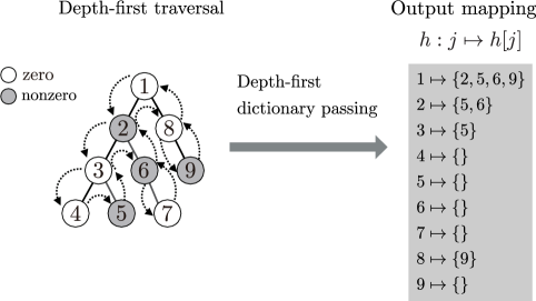
Figure 5: An example of depth-first dictionary passing. Depth-first dictionary passing is a procedure to produce the mapping $h$ on the right after the depth-first traversal of the tree on the left. Each $h[j]$ is the indices of nonzero nodes below node $j$.

In this subsection, we describe how to obtain $\underline{B}_{j}(t)$ and $\overline{B}_{j}(t)$ in Theorem 11 which are needed for computing $\theta(t+1)$ from $\theta(t)$. Since we already have the nonzero coordinates of $\theta(t)$ for the index subset $\{j\mid\theta(t)_{j}\neq 0\}$ at hand, these bounds are defined simply as the maximum and minimum of the finite candidates:

$$\underline{B}_{j}(t) :=\min_{l\in\{k\mid x_{k}\in\mathcal{T}(x_{j})\}}(\lambda_{2}-H(t)_{ll})\theta(t)_{l}=\min\left(0,\min_{l\in\{k\mid x_{k}\in\mathcal{T}(x_{j}),\theta(t)_{k}\neq 0\}}(\lambda_{2}-H(t)_{ll})\theta(t)_{l}\right),$$

$$\overline{B}_{j}(t) :=\max_{l\in\{k\mid x_{k}\in\mathcal{T}(x_{j})\}}(\lambda_{2}-H(t)_{ll})\theta(t)_{l}=\max\left(0,\max_{l\in\{k\mid x_{k}\in\mathcal{T}(x_{j}),\theta(t)_{k}\neq 0\}}(\lambda_{2}-H(t)_{ll})\theta(t)_{l}\right).$$

We can compute these values in a brute-force manner by checking $x_{j}\subseteq x_{k}$ for all $k$ such that $\theta(t)_{k}\neq 0$, but this is practically inefficient due to subgraph isomorphism test.

What we need instead is an efficient way to obtain, for each $j$, the index subset

$$\{k\mid x_{k}\in\mathcal{T}(x_{j}),\theta(t)_{k}\neq 0\}.$$ (9)

Recall that in order to obtain $\{j\mid\theta(t)_{j}\neq 0\}$, we traverse the enumeration tree $\mathcal{T}(\mathcal{G}_{n})$ to find all $j$ such that $T(\theta(t-1))_{j}\neq 0$ using the bounds in Theorem 11 (Figure 4). During this traversal, we can also record, for every visited node $x_{j}$, the mapping

$$j\mapsto\{k\mid x_{k}\in\mathcal{T}(x_{j}),T(\theta(t-1))_{k}\neq 0\}.$$ (10)

If we have this mapping, then we can recursively obtain (9) for each $j$ as

$$\{k\mid x_{k}\in\mathcal{T}(x_{j}),\theta(t)_{k}\neq 0\}$$

$$=\left(\{k\mid x_{k}\in\mathcal{T}(x_{j}),T(\theta(t-1))_{k}\neq 0\}\cup\{k\mid x_{k}\in\mathcal{T}(x_{j}),\theta(t-1)_{k}\neq 0\}\right)$$

$$\hskip 20.00003pt\cap\{k\mid\theta(t)_{k}\neq 0\}.$$ (11)

Hence in what follows, we present the procedure, which we call depth-first dictionary passing, to build the mapping of (10) over all necessary $j$. Figure 5 shows an example of depth-first dictionary passing for the search tree on the left (The output is shown on the right).

First, we define $\mathcal{T}_{\mathrm{visited}}(\mathcal{G}_{n})$ as the tree consisting of all visited nodes during the depth-first traversal of $\mathcal{T}(\mathcal{G}_{n})$ with pruning based on Theorem 11. Note that $\mathcal{T}_{\mathrm{visited}}(\mathcal{G}_{n})$ is a subtree of $\mathcal{T}(\mathcal{G}_{n})$, and it holds that $x_{j}\in\mathcal{T}_{\mathrm{visited}}(\mathcal{G}_{n})$ for all $x_{j}$ such that $T(\theta(t))_{j}\neq 0$. We then define an auxiliary mapping as

$$h^{\prime}(t):=\left\{(j\mapsto\{k\mid x_{k}\in\mathcal{T}(x_{j}),T(\theta(t))_{k}\neq 0\})\mid x_{j}\in\mathcal{T}_{\mathrm{visited}}(\mathcal{G}_{n})\right\}$$ (12)

with four operations of Get, Put, Keys, and DeleteKey: For a mapping $h:j\mapsto z$, Get returns the target $z$ of indicated $j$, which we write by $h[j]$. Put registers a new pair $(j\mapsto z)$ to $h$, which we write simply by $h[j]\leftarrow z$. Keys returns all registered keys in $h$ as $\text{{Keys}}(h)=\{j\mid(j\mapsto z)\in h\}$. DeleteKey deletes the pair $(j\mapsto z)$ indicated by $j$ from $h$ as $\text{{DeleteKey}}(h,j)=h-\{(j\mapsto z)\}$.

During the depth-first traversal of $\mathcal{T}(\mathcal{G}_{n})$ at time $t$, we keep a tentative mapping, $h_{\mathrm{tmp}}(t)$, to build $h^{\prime}(t)$ of (12) at the end. We start with an empty $h_{\mathrm{tmp}}(t)$. Then we update and pass $h_{\mathrm{tmp}}(t)$ to the next node of the depth-first traversal. In the pre-order operation, if we encounter $x_{j}\in\mathcal{T}_{\mathrm{visited}}(\mathcal{G}_{n})$ such that $T(\theta(t))_{j}\neq 0$, we add this $j$ to all $h_{\mathrm{tmp}}[i]$ for $i\in\text{{Keys}}(h_{\mathrm{tmp}})$ by $h_{\mathrm{tmp}}[i]\leftarrow h_{\mathrm{tmp}}[i]\cup\{j\}$. This informs all the ancestors that $T(\theta(t))_{j}\neq 0$. Then, we register $j$ itself to $h_{\mathrm{tmp}}$ by initializing as $h_{\mathrm{tmp}}[j]\leftarrow\{\}$. In the post-order operation, if we have $h_{\mathrm{tmp}}[j]\neq\{\}$, then it implies that $x_{j}$ has descendants $x_{k}\in\mathcal{T}(x_{j})$ such that $T(\theta(t))_{k}\neq 0$ and $k\in h_{\mathrm{tmp}}[j]$. Thus, this is an element of our target set $h^{\prime}(t)$, and we finalize the $j$-th element $h^{\prime}(t)[j]$ by setting $h^{\prime}(t)[j]\leftarrow h_{\mathrm{tmp}}[j]$. At this point, we also remove $j$ from $h_{\mathrm{tmp}}$ by DeleteKey$(h_{\mathrm{tmp}},j)$ because $j$ cannot be an ancestor of any forthcoming nodes in the subsequent depth-first traversal after $x_{j}$. In this way, we can obtain $h^{\prime}(t)$ defined in (12) at the end of traversal.

The depth-first dictionary passing finally gives us the mapping (9) as

$$h(t):=\left\{(j\mapsto\{k\mid x_{k}\in\mathcal{T}(x_{j}),\theta(t)_{k}\neq 0\})\mid x_{j}\in\mathcal{T}_{\mathrm{visited}}(\mathcal{G}_{n})\right\}$$

from $h^{\prime}(t-1),h(t-1)$ and the nonzero coordinates of $\theta(t)$ by using a recursive formula of (11). This also gives $\underline{B}_{j}(t)$ and $\overline{B}_{j}(t)$ in Theorem 11 which are needed for computing $\theta(t+1)$ from $\theta(t)$.

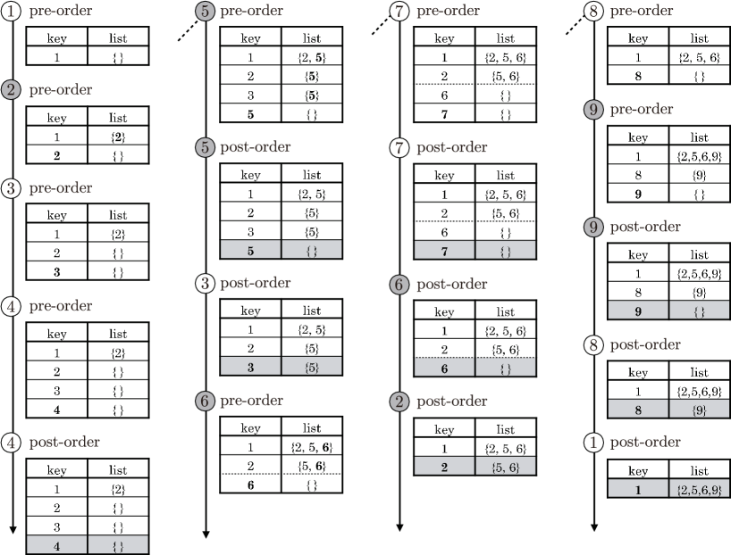
Figure 6: The transition of tentative mapping $h_{\mathrm{tmp}}$ in the depth-first dictionary passing in Figure 5. The order follows the depth-first order of traversal, and each shaded mapping at post-order operations constitutes the final output $h$. At the end of traversal, we have the mapping $h$ on the right in Figure 5 as the collection of all shaded mappings.

Figure 6 shows an example of building $h_{\mathrm{tmp}}$ (each key-list table) and registration to $h^{\prime}$ (shown as the shaded colored key-list pairs) for the case of Figure 5. First, we start a depth-first traversal from node $1$. In the pre-order operation at node $1$, we just register key $1$ to $h_{\mathrm{tmp}}$ as $h_{\mathrm{tmp}}[1]\leftarrow\{\}$. The next node $2$ is shaded, which indicates that $T(\theta(t))_{2}\neq 0$, then we inform node $2$ to all ancestors by $h_{\mathrm{tmp}}[1]\leftarrow h_{\mathrm{tmp}}[1]\cup\{2\}$ and also initialize as $h_{\mathrm{tmp}}[2]\leftarrow\{\}$. At node $3$ and $4$, we just add $h_{\mathrm{tmp}}[3]\leftarrow\{\}$ and $h_{\mathrm{tmp}}[4]\leftarrow\{\}$, but at node $4$, we also need the post-order operation of registering the mapping of $4$ to $h^{\prime}$ and then removing key $4$. As a result, at the shaded node of $5$, we have keys of $1,2$ and $3$ in $h_{\mathrm{tmp}}$. In the pre-order operation at node $5$, we add $5$ to all of these as $h_{\mathrm{tmp}}[1]\leftarrow h_{\mathrm{tmp}}[1]\cup\{5\}$, $h_{\mathrm{tmp}}[2]\leftarrow h_{\mathrm{tmp}}[2]\cup\{5\}$ and $h_{\mathrm{tmp}}[3]\leftarrow h_{\mathrm{tmp}}[3]\cup\{5\}$. In this way, we keep $h_{\mathrm{tmp}}$, and obtain $h^{\prime}$ at the end (as the set of the shaded key-list pairs in tables of Figure 6).

4.4 Algorithm

Figure 1 shows the pseudocode for the entire procedure.

  Algorithm:

  $\theta(0)\leftarrow 0$;

Build empty $h,h^{\prime}$;

for $t=0,1,2,\dots$ do

       Build an empty $hes,h_{\mathrm{tmp}}$;

       foreach $i\in\{i\mid\theta(t)_{i}\neq 0\}$ do $hes[i]\leftarrow H(t)_{ii}$;

      ;

       foreach $x_{j}\in\mathcal{T}(\mathcal{G}_{n})$ in the depth-first traversal do

             begin pre-order operation

                   Compute $T(\theta(t))_{j}$ ;

                   // by Lemma 10

                   if $T(\theta(t))_{j}\neq 0$ then

                         foreach $i\in$Keys$(h_{\mathrm{tmp}})$ do $h_{\mathrm{tmp}}[i]\leftarrow h_{\mathrm{tmp}}[i]\cup\{j\}$;

                        ;

                        

                   end if

                  $h_{\mathrm{tmp}}[j]\leftarrow\{\}$;

                   $h[j]\leftarrow(h[j]\cup h^{\prime}[j])\cap\{i\mid\theta(t)_{i}\neq 0\}$ ;

                   // by formula (11)

                   if $h[j]=\{\}$ then

                         $\underline{B}_{j}\leftarrow 0,\overline{B}_{j}\leftarrow 0$;

                        

                  else

                         $\overline{B}_{j}\leftarrow\max\left\{\max_{k\in h[j]}\{(\lambda_{2}-hes[k])\theta(t)_{k}\},0\right\}$;

                         $\underline{B}_{j}\leftarrow\min\left\{\min_{k\in h[j]}\{(\lambda_{2}-hes[k])\theta(t)_{k}\},0\right\}$;

                        

                   end if

                  Compute $\overline{L}_{j},\underline{L}_{j}$ ;

                   // by Lemma 8

                   if $\max\{\overline{L}_{j}+\overline{B}_{j},-\underline{L}_{j}-\underline{B}_{j}\}\leqslant\lambda_{1}$  then // by Theorem 11

                        Prune $\mathcal{T}(x_{j})$;

                  else

                        Visit children of $x_{j}$;

                   end if

                  

             end

            

            begin post-order operation

                   if $h_{\mathrm{tmp}}[j]\neq\{\}$  then

                         $h^{\prime}[j]\leftarrow h_{\mathrm{tmp}}[j]$;

                        

                   end if

                  DeleteKey$(h_{\mathrm{tmp}},j)$;

                  

             end

            

       end foreach

      $d(t)_{i}\leftarrow T(\theta(t))_{i}-\theta(t)_{i}$ for $i\in\{i\mid T(\theta(t))_{i}\neq 0\vee\theta(t)_{i}\neq 0\}$;

       Gauss-Southwell-r: $d(t)_{i}\leftarrow 0$ for $i$ such that $|d(t)|_{i}\leqslant v(t)\cdot\|d(t)\|_{\infty}$;

       Armijo: $\theta(t+1)\leftarrow\theta(t)+\alpha d(t)$ ;

       // by formula (7)

       Convergence test: if $\|H(t)d(t)\|_{\infty}\leqslant\epsilon$ then quit;

      ;

      

end for

 

Algorithm 1 The entire algorithm for solving Problem 1.

5 Numerical Results

The proposed approach not only estimates the model parameters, but also simultaneously searches and selects necessary subgraph features from all possible subgraphs. This is also the case with existing approaches such as Adaboost (Kudo et al., 2005) and LPBoost (Saigo et al., 2009).

In this section, we thus numerically investigate the following three points to understand the difference from these previously developed methods.

• Convergence properties: Contribution of the selected subgraph features at each iteration to the convergence to the optimal solution.

• Selected features: Difference in the final selected subgraph features of three methods.

• Search-tree size: Enumeration tree size at each iteration for searching necessary subgraph features.

In order to systematically analyze these three points, we develop a benchmarking framework where we can control the property, size, and number of graph samples as well as we can measure the training and test error of the model at each iteration. We generate two sets of graphs by probabilistically combining a small random subgraphs as unobserved discriminative features, and prepare a binary classification task of these two sets in a supervised-learning fashion (the details are described in Section 5.1). This generative model allows us to simulate the situation where observed graphs have discriminative subgraph features behind, and we can compare the selected subgraph features by each learning algorithm to these unobserved “true” features. In addition, we can also evaluate not only the training error but also the test error. These two points are required since our goal here is to understand the basic properties for convergence and subgraph feature selection. For this binary classification task, we compare the following three methods. We set the same convergence tolerance of $10^{-3}$ for both logistic regression and LPBoost.

1. 1-norm penalized logistic regression for graphs (with the proposed learning algorithm). Logistic regression is one of the most standard methods for binary classification, which is often considered as a baseline for performance evaluation. We optimize the logistic regression with 1-norm regularization by the proposed algorithm with $\lambda_{2}=0$ and

   $$L(y,\mu)=y\log(1+\exp(-\mu))+(1-y)\log(1+\exp(\mu)),\quad y\in\{0,1\}$$ (13)

   (or equivalently $L(y,\mu)=\log(1+\exp(-y\mu)),y\in\{-1,1\}$). For the loss function of (13), we have the derivative and the Hessian as

   $$\frac{\partial L(y,\mu)}{\partial\mu}=\frac{1}{1+\exp(-\mu)}-y,\qquad\frac{\partial^{2}L(y,\mu)}{\partial^{2}\mu}=\frac{1}{1+\exp(-\mu)}\cdot\frac{1}{1+\exp(\mu)},$$

   respectively. Moreover, according to the example of Yun and Toh (2011), we set

   $$H(t)_{jj}:=\min\left\{\max\{\nabla^{2}f(\theta(t))_{jj},10^{-10}\},10^{10}\right\}$$

   and

   $$\sigma=0.1,c=0.5,\gamma=0,\alpha_{\mathrm{init}}(0)=1,\alpha_{\mathrm{init}}(t)=\min\left\{\frac{\alpha(t-1)}{c^{5}},1\right\},v(t)=0.9.$$

   Note that at each iteration, our optimization method adds multiple subgraph features at once to the selected feature set, which is different from the following two methods.

2. Adaboost for graphs (Kudo et al., 2005). This is a learning method by a sparse linear model over all possible subgraphs by adding the single best subgraph feature to improve the current model at each step, by using the framework of Adaboost. Adaboost can be asymptotically viewed as a greedy minimization of the exponential loss function.

3. LPBoost for graphs (Saigo et al., 2009). Adaboost adds a single feature at each iteration, and does not update the indicator coefficients already added to the current model. By contrast, LPBoost updates all previous coefficients at each iteration of adding a new single feature. This property is known as the totally-corrective property which can accelerate the convergence. LPBoost minimizes the hinge loss function with 1-norm regularization. Since the hinge loss is not twice differentiable, LPBoost is complementary to our framework.

We emphasize that classification performance depends on the objective function and has nothing to do with the optimization method. Our interest is not necessarily in comparing the performance and property of Logistic regression, Adaboost, and LPBoost, which have long been discussed in the machine-learning community. Rather, as we already mentioned above, we are interested in the convergence properties, selected subgraph features, and search-tree sizes along with adaptive feature learning from all possible subgraph indicators.

L1-LogReg was implemented by C++ entirely from the scratch. For Adaboost and LPBoost, we used the implementations in C++ by Saigo et al. (2009) which are faster than other implmentations. The source code was obtained from author’s website, and we added a few lines carefully to count the number of visited nodes. We also set minsup=1 and maxpat=$\infty$ in the original code, to run Adaboost and LPBoost over all possible subgraph features.

5.1 Systematic Binary Classification Task

Figure 2 presents the procedure for generating two set of graphs. These two sets correspond to graph sets (i) and (ii) in Figure 7 which are generated by a consistent probabilistic rule: each graph in (i) includes each subgraph feature in subgraph set (A) with a probability of $p_{1}$ and similarly each feature in (B) with $q_{1}$; Each graph in (ii) includes each subgraph feature in (A) with a probability of $p_{2}$ and each feature in (B) with $q_{2}$ (as summarized on the right in Figure 7), where a seed-graph pool of (A) and (B) are also generated randomly. When we set $p_{1}>q_{1}$ and $q_{2}>p_{2}$, we can assume $V$ and $W$ dominant subgraph features that can discriminate between (i) and (ii). By using these two sets (i) and (ii) as positive and negative samples respectively, we define a systematic binary classification task with control parameters $V,W,N,M,p_{1},p_{2},q_{1},q_{2}$ and the Poisson mean parameter. This procedure, which was inspired by Kuramochi and Karypis (2004), first generates $V+W$ random graphs as $X:=\{x_{1},x_{2},\dots,x_{V+W}\}$ for a seed-graph pool, and then generates $N+M$ output graphs by selecting and combining these seed graphs in $X$ with the probabilistic rule: as indicated in Figure 7, the probability that output graph $i$ contains subgraph feature $j$ or not ($I_{i,j}=1$ or $0$) is determined block by block. To generate each output graph, the selected seed subgraphs are combined by the procedure combine in Figure 3 which finally produces the output graphs (i) and (ii) having the data matrix in Figure 7. The mean parameter for the Poisson distribution is set to $3$, and the number of node and edge labels to $5$ throughout the numerical experiments.

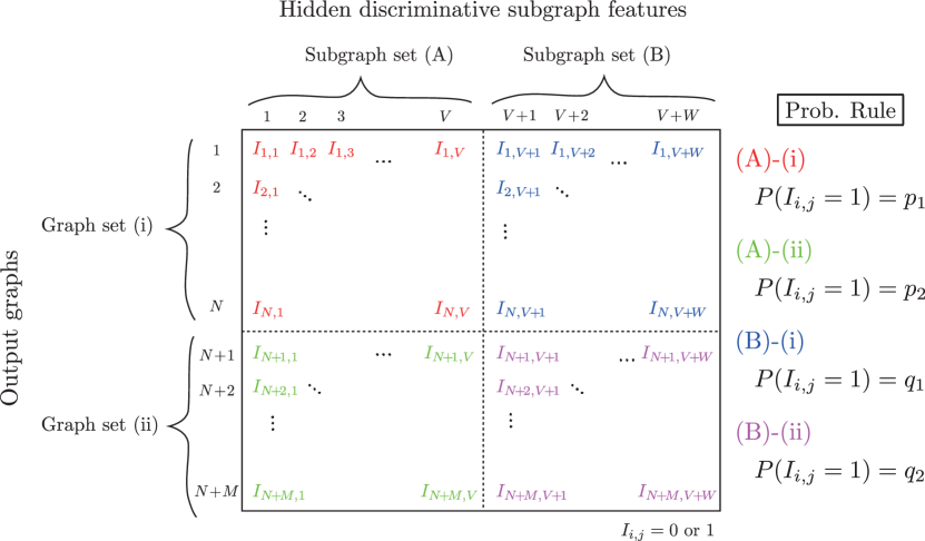
Figure 7: The data matrix: two graph sets (i) and (ii) which are generated by the procedure in Figure 2. These graphs are generated by combining graphs in random subsets of a seed-graph pool of (A) and (B) with the procedure in Figure 3. Each subset is randomly generated, following the probabilistic rule (on the right) that is defined for each block.

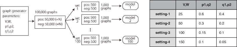
Figure 8: The scheme and settings of data generation for numerical evaluations. We generated 100 sets of 1,000 random graphs consisting of 500/500 graphs for (i)/(ii) in Figure 7, respectively, sharing the same generative rule. Thus, we can examine the test error of model $i$ using set $j$ ($i\neq j$) in addition to the training error.

Table 1: Statistics on the generated datasets.

data set	# graphs	# edges			# nodes
		max	min	avg	max	min	avg
setting-1	100,000	193	49	119.54	162	44	101.53
setting-2	100,000	219	32	120.28	182	28	103.03
setting-3	100,000	246	33	115.91	202	29	100.78
setting-4	100,000	221	25	104.46	187	23	90.61

  Algorithm:

  Generate $V+W$ Poisson random numbers $a_{1},a_{2},\dots,a_{V+W}$ (resample if $a_{i}<2$);

Initialize dictionary $d$;

Initialize seed-graph pool $X\leftarrow\{\}$;

for $i=1,2,\dots,V+W$ do

       Generate a graph $g$ with two node and an edge between them. (node and edge are labeled at random);

       repeat $a_{i}$ times do

             Select a node $\alpha$ from $g$ at random;

             Select one of the two choice at random (to ensure the connectivity of $g$);

             i) Add an edge from $\alpha$ to a node of $g$ that is not adjacent to $\alpha$;

             ii) Add a new node $\alpha^{\prime}$ to $g$ and an edge between $\alpha$ and $\alpha^{\prime}$;

            

       end

      if $\mathtt{MinDFSCode}(g)$ in $d$ then

            continue;

       else

             Register $\mathtt{MinDFSCode}(g)$ to $d$;

             $X\leftarrow X\cup\{g\}$;

            

       end if

      

end for

Set the first $V$ graphs in $X$ as $A$, and the last $W$ graphs in $X$ as $B$;

repeat $N$ times to generate $N$ positive samples do

       Select $S_{V}\subseteq A$ with $P(x_{i}\in S_{V})=p_{1}$ for $x_{i}\in A,i=1,2,\dots,V$;

       Select $S_{W}\subseteq B$ with $P(x_{i}\in S_{W})=q_{1}$ for $x_{i}\in B,i=1,2,\dots,W$;

       $g\leftarrow$combine($S_{V}\cup S_{W}$);

       Add $g$ to a set of positive examples;

      

end

repeat $M$ times to generate $M$ negative samples do

       Select $S_{V}\subseteq A$ with $P(x_{i}\in S_{V})=p_{2}$ for $x_{i}\in A,i=1,2,\dots,V$;

       Select $S_{W}\subseteq B$ with $P(x_{i}\in S_{W})=q_{2}$ for $x_{i}\in B,i=1,2,\dots,W$;

       $g\leftarrow$combine($S_{V}\cup S_{W}$);

       Add $g$ to a set of negative examples;

      

end

 

Algorithm 2 The procedure for class-labeled random graph generation.

  Function: combine($x_{1},x_{2},x_{3},\dots$)

  $g^{\prime}\leftarrow x_{1}$;

foreach $g_{i}$ in $x_{2},x_{3},\dots$ do

       Select a node of $g^{\prime}$ and a node of $g_{i}$ at random;

       Add an edge between them, and replace $g^{\prime}$ by the combined graph;

      

end foreach

return $g^{\prime}$  

Algorithm 3 The algorithm for combining several graphs into a single connected graph.

5.2 Evaluating Learning Curves

We first investigate the convergence property by the learning curves of the three methods on the same dataset. Figure 8 shows a schematic manner of generating an evaluation dataset by using the random graph generator in Figure 2. First we generate 100,000 graphs with the fixed parameters of $p_{1},p_{2},q_{1}$, and $q_{2}$, and then divide them into 100 sets, each containing 1,000 graphs (500 positives and 500 negatives). Out of each set of 1,000 graphs, we train the model by either of Adaboost, LPBoost, and 1-norm penalized logistic regression (denoted by L1-LogReg hereafter). We estimate the expected training error by computing each training error of model $i$ with data set $i$ that is used to train the model, and averaging over those 100 values obtained from 100 sets. Moreover, since all 100 sets share the same probabilistic rule behind its generation, we can also estimate the expected test error by first randomly choosing 100 pairs of set $i$ and model $j$ ($i\neq j$), and computing the test error of the model $i$ with data set $j$ that is not used to train the model, and averaging over those 100 values obtained from 100 pairs. We use the same fixed 100 pairs for evaluating all three methods of Adaboost, LPBoost, and L1-LogReg. Since we have the intermediate model at each iteration, we can obtain the training and test error at each iteration, which gives us the learning curves of the three methods regarding the training error as well as the test error. We use four different settings for control parameters, which are shown in Figure 8. Table 1 shows the statistics on the datasets generated by these four settings. It should be noted that when we draw an averaged learning curve, we need to perform $100$ trainings and $100$ testings for $1,000$ graphs at each iteration. For example, the learning curves of $150$ iterations requires $150\times 100$ trainings and $150\times 100$ testings for $1,000$ graphs.

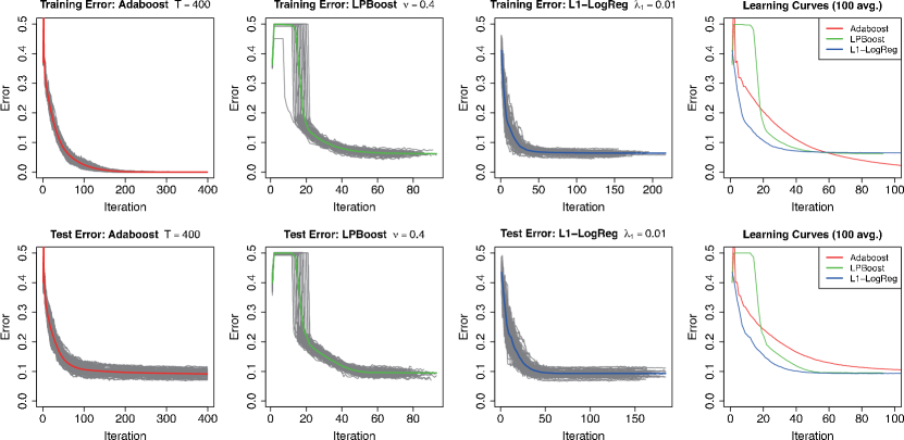
Figure 9: Learning curves for setting-1 (average over 100 trials).

First, for each setting of the data generation in Figure 8, the estimated learning curves are shown in Figures 9 (setting-1), 10 (setting-2), 11 (setting-3), and 12 (setting-4). On the left three panels in each figure, we show 100 learning curves from each of 100 sets, and their averaged curves (in red color). On the right-most panel, we show only three averaged curves for comparison.

From these figures, we can first see that the convergence rate was clearly improved by the proposed algorithm compared to Adaboost and LPBoost. Also we can see that LPBoost accelerated the convergence rate of Adaboost by totally corrective updates. The convergence behavior of LPBoost was unstable at the beginning of iterations, which was already pointed out in the literature (Warmuth et al., 2008a, b), whereas Adaboost and the proposed method were more stable. LPBoost however often achieved slightly higher accuracy than L1-LogReg and Adaboost, implying that the hinge loss function (LPBoost) fits better to the task compared to the logistic loss (L1-LogReg) or the exponential loss (Adaboost).

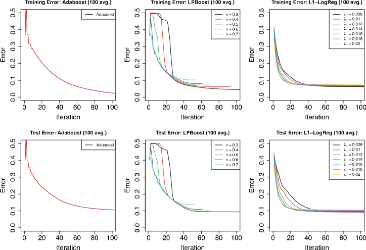
Figure 13: Average learning curves for different parameters (setting-1).

Second, Figures 13 (setting-1), 14 (setting-2), 15 (setting-3), and 16 (setting-4) show the estimated learning curves (averaged over 100 sets) for different parameters of each learning model. Adaboost has only one parameter for the number of iterations, and the difference in settings did not affect the learning curves, while LPBoost and L1-LogReg have a parameter for regularization. The parameter of L1-LogReg affects the training error and test error at convergence, but in any cases, the result showed more stable and faster convergence than the other two methods. Also we could see that the parameter of LPBoost also affected the instability at the beginning of iterations. Regarding performance, LPBoost was in many cases slightly better than the other two, but the error rate at the best parameter tuning was almost the same in practice for this task.

5.3 Evaluating the difference in selected subgraph features

Third, we compared the resultant selected subgraph features at convergence of the three models. To make this evaluation as fair as possible, we used setting-2 with the parameter of 325 for Adaboost, 0.335 for LPBoost, and 0.008 for L1-LogReg, which were all carefully adjusted so as to have almost the same number of non-redundant selected features. As shown in Table 2, we had about 240 features on average, and we also observed that the three methods gave mostly the same test error of around 0.17. We could see that the original dataset of setting-2 was generated by combining 100 small graphs in the seed-graph pool ($V+W=100$), but the number of learned features in Table 2 exceeded the number of features to generate the data. This is because the presence of any graph can be confirmed by the presence of smaller co-occurring subgraphs that would be contained in unseen samples with high probability. For the setting of Table 2, Figure 17 shows the number of features with nonzero coefficients at each iteration (averaged over 100 data sets), all of which converged to around 240 features. The number of features of L1-LogReg increased quickly at the beginning of iterations and then slightly dropped to the final number. In addition, the variance of the number was larger than Adaboost and LPBoost. On the other hand, the number of features of Adaboost and LPBoost increased almost linearly. Note that we count only non-redundant features by unifying the identical features that are added at different iterations. We also ignore features with zero coefficients.

Next, we checked the size of individual subgraph features, which is the number of edges of each subgraph feature. In Figure 18, we show the size distribution of subgraph features in the seed-graph pool in the left-most panel that is used to generate the data, and those of Adaboost, LPBoost, and L1-LogReg to the right. Interestingly, even though the number of features ($\approx 240$) and the performance of the three methods ($\approx 0.17$) were almost similar under the setting of Table 2, the selected set of subgraph features was quite different. First we can conclude that these learning algorithms do not directly choose the discriminative subgraph features. Compared to the original subgraphs stored in the seed-graph pool (up to size 7), all three methods chose much smaller subgraphs and tried to represent the data by combining those small subgraphs. In particular, Adaboost and LPBoost focused on selecting the subgraph features, where their size was less than and equal to three, mostly the subgraph feature of size two (graphs with three nodes and two edges). By contrast, L1-LogReg had more balanced size distribution, and the most frequent subgraph features were of size three. Figure 19 shows the number of overlapped subgraph features between different methods (averaged over 100 sets). Figure 18 might give a misleading impression that the selected features of Adaboost and LPBoost would be similar when the obtained number of features is similar. Yet they are remarkably different as we see in Figure 19. By looking more closely, LPBoost and Adaboost shared a much larger number of features than those between either of them and L1-LogReg. For example, out of 240, 71.8 + 64.42 = 136.22 features are shared between Adaboost and LPBoost, whereas 91.71 and 99.15 features are shared between L1-LogReg and Adaboost, and between L1-LogReg and LPBoost, respectively. This implies that L1-LogReg captured a more unique and different set of subgraph features compared to the other two, as already implied by the size distribution of Figure 18, while as shown in Figure 19, the overlap between the subgraph features obtained by L1-LogReg and the seed-graph pool was larger than that by Adaboost and LPBoost. This suggests that L1-LogReg optimized by our method captured subgraph features which are relevant to given training data, which would be more advantageous when we try to interpret the given data.

5.4 Evaluating the difference in search space size

Lastly, Figure 20 shows the size of search space in the three methods, i.e. the number of visited nodes in the enumeration tree, $\mathcal{T}_{\mathrm{visited}}(\mathcal{G}_{n})$. Adaboost and LPBoost start with relatively shallower traversal at the beginning of iterations, and then search deeper as the iteration proceeds. On the other hand, the proposed method starts with deep search, and then updates only a few necessary coefficients by further narrowing search at the subsequent iterations. Thus, intensive search of necessary features was done within the beginning of iterations, and the the number of nonzero coefficients that need to be updated was small at the later iterations.

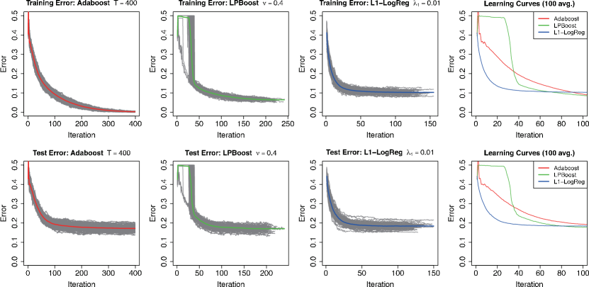
Figure 10: Learning curves for setting-2 (average over 100 trials).

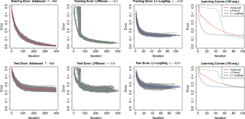
Figure 11: Learning curves for setting-3 (average over 100 trials).

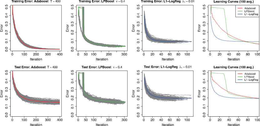
Figure 12: Learning curves for setting-4 (average over 100 trials)).

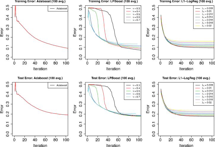
Figure 14: Average learning curves for different parameters (setting-2).

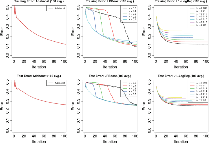
Figure 15: Average learning curves for different parameters (setting-3).

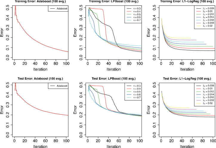
Figure 16: Average learning curves for different parameters (setting-4).

Table 2: Statistics for setting-2 at convergence (average over 100 trials).

method	param	# feat	# iter	error
				(train)	(test)
Adaboost	325	239.94 $\pm$ 8.50	325	0.0068	0.1736
LPBoost	0.335	239.69 $\pm$ 21.80	275.91	0.0405	0.1704
L1-LogReg	0.008	239.36 $\pm$ 29.16	122.52	0.0931	0.1758
		$\approx$ 240			$\approx$ 0.17

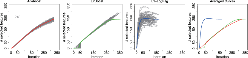
Figure 17: The number of unique subgraph features along the iterations.

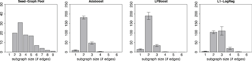
Figure 18: Distribution of the size of non-redundant subgraph features (average over 100 trials).

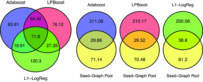
Figure 19: The number of isomorphic subgraph features (average over 100 trials).

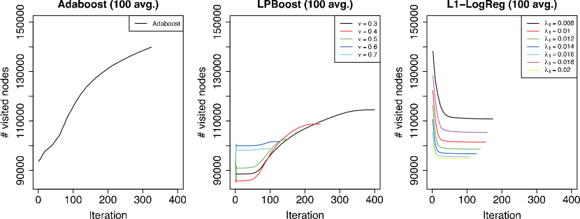
Figure 20: The number of visited nodes in the enumeration tree.

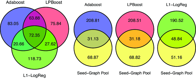
Figure 21: The number of overlapping subgraph features by the equivalence classes (average over 100 trials).

Table 3: Classification accuracy for the CPDB dataset (10-fold CV).

method		param	ACC		# feat
			(train)	(test)
L1-LogReg		0.005	0.813	0.774	80.3
Adaboost		500	0.945	0.772	180.3
LPBoost		0.4	0.895	0.784	101.1
glmnet	FP2	0.02	0.828	0.739	1024
(L1-LogReg)	FP3	0.03	0.676	0.628	64
	FP4	0.02	0.785	0.721	512
	MACCS	0.01	0.839	0.771	256

Table 4: Performance and search-space size for the CPDB dataset (10-fold CV).

method	param	ACC		# feat	# iter	time	# visited		% skipped
		(train)	(test)			(sec)	avg	max	avg	max
L1-LogReg	0.004	0.825	0.755	95.0	57.5	8918.94	54250.2	415079.5	96.17%	96.22%
	0.005	0.813	0.774	80.3	62.3	2078.88	31472.4	128906.7	90.40%	90.57%
	0.006	0.803	0.762	67.6	66.6	1012.93	23354.2	85428.7	85.74%	85.88%
	0.008	0.779	0.750	50.9	50.6	277.69	16587.7	46213.1	76.78%	76.82%
	0.010	0.756	0.733	39.1	46.4	97.29	12524.3	26371.4	69.95%	70.02%
Adaboost	600	0.950	0.769	190.0	600.0	40.67	67907.2	108425.0
	500	0.945	0.772	180.3	500.0	36.21	61643.9	107421.7
	400	0.938	0.769	168.8	400.0	29.38	53657.1	96412.1
LPBoost	0.3	0.939	0.748	141.4	185.9	16.02	19977.8	41921.5
	0.4	0.895	0.784	101.1	126.4	7.76	15431.7	28905.9
	0.5	0.858	0.767	67.1	80.2	4.39	12242.6	22290.1

6 Discussion

In this section, we point out and discuss some new issues about learning from graphs that we have noticed during developing the proposed framework.

6.1 Bias towards selecting small subgraph features

As we see in Figure 17, all three models of Adaboost, LPBoost, and L1-LogReg tend to choose smaller subgraph features. The generated graphs by the algorithm of Figure 2 are based on combining the graphs in a random seed-graph pool. The size of graphs in the seed-graph pool follows a Poisson distribution, which is shown in the histogram in Figure 17, which shows the distributions of subgraphs captured by the three methods as well. The distributions by the three methods show that small subgraphs were captured, because large subgraph features can be identified by checking multiple smaller subgraphs, and moreover small subgraphs would occur in the data with higher probability than larger ones. Yet there is still remarkable difference in characteristics between the subgraph features of Adaboost, LPBoost, and L1-LogReg even when the performance are similar as in Table 2. That is, a closer look shows that Adaboost and LPBoost choose subgraphs of size two rather than size three, and L1-LogReg choose subgraphs of size both two and three. This means that comparing to a random seed-graph pool, L1-LogReg comes with more balanced size of subgraph features, whereas Adaboost and LPBoost mostly choose the subgraphs of size two only. Also note that the features of Adaboost and LPBoost are similar in size (Figure 18), but they are still very different (Figure 19). This finding would suggest that we need to be careful about the result when we interpret the learned subgraphs in real applications.

6.2 High correlation and equivalence class by perfect multicollinearity of subgraph indicators

The design matrix of Figure 1 may have high correlations between column vectors (or regressors). When subgraph features $x_{i}$ and $x_{j}$ are very similar, (for example, only one or two edges are different between them), the corresponding subgraph indicators $I(x_{i}\subseteq g)$ and $I(x_{j}\subseteq g)$ would take very similar values. Moreover, the number of samples are generally far less than the number of possible subgraph features. Therefore, we can have many exactly identical column vectors that correspond to different subgraph features, which causes perfect multicollinearity.

In most practical cases, we have a particular set of subgraph features, say $X$, such that any $x\in X$ has the same Boolean vector of $I_{\mathcal{G}_{n}}(x)$. These subgraph features form an equivalence class

$$[x]:=\{x^{\prime}\in\mathcal{X}(\mathcal{G}_{n})\mid I_{\mathcal{G}_{n}}(x^{\prime})=I_{\mathcal{G}_{n}}(x)\},$$

where any representative subgraph feature $x$ has the same $I_{\mathcal{G}_{n}}(x)$. Note that two graphs with very different structures can be in the same equivalence class if they perfectly co-occur (For example, disconnected-subgraph patterns).

Therefore, for given $x_{i},x_{j}\in[x]$, we cannot distinguish if either of two subgraph indicators is better than the other, just by using $\mathcal{G}_{n}$. A heuristics is that the smallest subgraph in $[x]$ might be good as the representative subgraph, because smaller subgraphs are expected to occur in unseen graphs with a higher probability than that of larger ones. This point should be carefully treated when we are interested in interpreting the selected set of subgraph features for the application purpose. We can always have many other candidates in the equivalence class that has exactly the same effect as a subgraph feature.

The existing methods such as Adaboost and LPBoost add a single best subgraph feature at each iteration with branch and bound, and thus usually ignore this problem, because they just take the first found best subgraph. On the other hand, the proposed method allows to add multiple subgraph features at each iteration. Hence we need to handle this point explicitly. In this paper, for easy comparisons, we just take the first found subgraph $x$ (following the other methods) and ignore the subsequently found subgraph in the same equivalence class $[x]$ by a hashing based on $I_{\mathcal{G}_{n}}(x)$. This is simply because in this paper we are interested in the number of unique subgraphs. However we can output the complete set of the equivalence classes and analyze them when we are interested in interpreting the selected subgraphs. In addition, when we are interested in prediction performance only, we can instead use 2-norm regularization in our framework of Problem 1 to average over highly correlated features, although this method may increase the number of selected subgraph features.

Lastly, it should be noted that this equivalence class problem, being caused by perfect multicollinearity, might cast a question regarding the validity of comparing feature sets by graph isomorphism as was done in Section 5.3 and Figure 19. We conducted the same experiments by replacing the isomorphism test with an equivalence-class test based on the identity of $I_{\mathcal{G}_{n}}(x)$. The result is shown in Figure 21 and, from the comparison between Figures 19 and 21, we can confirm that our discussion in Section 5.3 would be still valid even when we take the equivalence class into account.

6.3 Performance on real dataset: The CPDB dataset

Despite the faster convergence in theory, our straightforward implementation of the algorithm of Figure 1 can be slow or even hard to compute for real-world datasets, at least in the current form. Thus future work includes improving the practical running time by pursuing more efficient algorithms and data structures.

In order to discuss this point, we show the performance result for a real dataset. We use the mutagenicity data for carcinogenic potency database (CPDB) compounds (Helma et al., 2004), which consists of 684 graphs (mutagens: 341, nonmutagens: 343) for a binary classification task. This dataset has been widely used for benchmarking (See, for example, Saigo et al. (2009)). Table 3 shows the comparison result of the classification accuracy (ACC) and the number of obtained subgraph features to attain that accuracy. We included a standard method in chemoinformatics as a baseline, in which we first computed the fingerprint bit vector and then applied standard 1-norm penalized logistic regression optimized by glmnet (Friedman et al., 2010) to the fingerprint. For fingerprints, we used four different fingerprints, FP1, FP2, FP3, and MACCS, generated by Open Babel. In terms of classification performance, L1-LogReg achieved similar accuracy to the best one by Adaboost and LPBoost with a much smaller number of subgraph features, whereas our method examined a larger search space than Adaboost and LPBoost as we see in Table 4. Table 4 shows the detailed statistics behind Table 3, where “time (sec)”, “# visited” and “% skipped” denote the CPU time in seconds, the number of visited nodes in the enumeration tree, and the percentage of skipped nodes due to perfect multicollinearity, respectively. Note that this CPU time cannot be a consistent measure, because the implementations of Adaboost and LPBoost maintain (or cache) the whole enumeration tree in the main memory (See Section 2.2 in Saigo et al. (2009)), whereas we did not use such implementation techniques. In this light the number of visited nodes would be the only measure to methodologically compare methods in Table 4 with each other.

When we focus on our method only, from the results of “time (sec)”, we can find that we need to decrease the regularization parameter $\lambda_{1}$ to a very small value, which would directly loosen the pruning condition of Theorem 11. As a result, the CPU time grows exponentially as the size of search space increases. One interesting point however is that as shown in “% skipped”, the redundant visits constitute a significant fraction of the total number of visits, which entails an exponentially long running time. If we can remove this bottleneck by skipping these unnecessary visits in some way, the performance can be largely improved. Another interesting point is that our framework needed the longest time at the first iteration as shown in Figure 20, but after several iterations the search-space size quickly decreases. If we adopt some warm start such as a continuation (homotopy) procedure (Yun and Toh, 2011; Wen et al., 2010; Hale et al., 2008a, b), it would also improve the performance. It would be future work to provide more realistic implementation by improving these points from algorithmic viewpoints.

6.4 Correctness of implementations: How should we debug them?

It is generally hard to make sure that a learning algorithm for graphs works correctly. There is no easy way to visualize a large set of graphs and subgraph features in a consistent form. This originates from the difficulty to visually find out graph isomorphism and subgraph isomorphism. Thus it would be an important problem how to check the correctness of the implemented algorithm. We know that the complete check is impossible in practice, and thus here we simply emphasize the importance of careful double check with systematically generated dataset.

For example, our implementation, fully written in C++ from the scratch, is based on the gSpan algorithm to implicitly build and traverse an enumeration tree $\mathcal{T}(\mathcal{G}_{n})$. We ensure that our implementation of gSpan works in the exactly same way to three other existing implementations with randomly generated graphs of various types. Similarly, we ensure that our implementation of Figure 1 works as expected using a simple double check as follows. When we limit the enumeration tree down to the $i$-th level, it is relatively easy to enumerate all bounded-size subgraphs in $\mathcal{X}(\mathcal{G}_{n})$ to a certain level of $i$. Given the results in Figure 18, even if we can check only up to $i=5$ or so, it should be valuable to check the identity to the case where we first generate the data matrix explicitly and apply the block coordinate gradient descent to the data matrix. Thus, for this level-limited enumeration tree up to the $i$-th level, we can explicitly generate the data matrix in the form of Figure 1. Applying the block coordinate gradient descent to this matrix is supposed to produce exactly the same coefficients and function values at each iteration as those which can be obtained when we limit $\mathcal{T}(\mathcal{G}_{n})$ by size. Using the original implementation of block coordinate gradient descent by Yun and Toh (2011), we double-check that the nonzero coefficient values and their indices are exactly the same at each iteration as our implementation with the level limitation. In addition, we double-check by applying glmnet (Friedman et al., 2010) to the data matrix and confirming if the values of the objective function at convergence are the same (because both glmnet and block coordinate gradient descent can be applied to the same problem of 1-norm penalized logistic regression). Note that glmnet in R first automatically standardizes the input variables, and thus we need to ignore this preprocessing part.

7 Conclusions

We have developed a supervised-learning algorithm from graph data—a set of graphs—for arbitrary twice-differentiable loss functions and sparse linear models over all possible subgraph features. To date, it has been shown that we can perform, under all possible subgraph features, several specific types of sparse learning such as Adaboost (Kudo et al., 2005), LPBoost (Saigo et al., 2009), LARS/LASSO (Tsuda, 2007), and sparse PLS regression (Saigo and Tsuda, 2008). We have investigated the underlying idea common to these preceding studies, including that we call Morishita-Kudo bounds, and generalized this idea to a unifying bounding technique for arbitrary separable functions. Then, combining this generalization with further algorithmic considerations including depth-first dictionary passing, we have showed that we can solve a wider class of sparse learning problems by carefully carrying out block coordinate gradient descent over the tree-shaped search space of infinite subgraph features. We then numerically studied the difference from the existing approaches in a variety of viewpoints, including convergence property, selected subgraph features, and search-space sizes. As a result, from our experiments, we could observe several unnoticed issues including the bias towards selecting small subgraph features, the high correlation structures of subgraph indicators, and the perfect multicollinearity caused by the equivalence classes. We believe that our results and findings contribute to the advance of understanding in the field of general supervised learning from a set of graphs with infinite subgraph features, and also restimulate this direction of research.

Appendix A1: Proof of Lemma 10

For applying coordinate descent to (6), we first set only the $j$-th element of $\theta$ free, i.e. $\theta_{j}=z$, and fix all the remaining elements by the current value of $\theta(t)$ as $\theta_{k}=\theta(t)_{k}$ for all $k\neq j$. Then, since (6) can be written as

$$\arg\min_{\theta_{1},\theta_{2},\dots}\biggl{[}\,\,\sum_{k=0}^{\infty}\nabla f(\theta(t))_{k}(\theta_{k}-\theta(t)_{k})+\frac{1}{2}\sum_{k=0}^{\infty}\sum_{l=0}^{\infty}H(t)_{kl}(\theta_{k}-\theta(t)_{k})(\theta_{l}-\theta(t)_{l})+\sum_{k=1}^{\infty}\lambda_{1}|\theta_{k}|\,\,\biggr{]},$$

we have the following univariate (one-dimensional) optimization problem for $z$

$$T(\theta(t))_{j}=\arg\min_{z}\biggl{[}\,\,\nabla f(\theta(t))_{j}(z-\theta(t)_{j})+\frac{1}{2}H(t)_{jj}(z-\theta(t)_{j})^{2}+\lambda_{1}|z|\,\,\biggr{]}.$$ (14)

On the other hand, for any $a\geqslant 0$, completing the square gives us

$$\arg\min_{z\in\mathbb{R}}\bigl{[}\,\,az^{2}+bz+c+\lambda|z|\,\,\bigr{]}=\begin{cases}-\frac{1}{2a}(b+\lambda)&b<-\lambda\\ -\frac{1}{2a}(b-\lambda)&b>\lambda\\ 0&-\lambda\leqslant b\leqslant\lambda.\end{cases}$$ (15)

Then, by rewriting (14) in the form of (15), we obtain the result in the lemma.

Appendix A2: Proof of Theorem 11

Let $L^{\prime}_{\mu}(y,\mu):=\partial L(y,\mu)/\partial\mu$. Then since $\partial\mu(g_{i},\theta(t))/\partial\theta(t)_{k}=I(x_{k}\subseteq g_{i})$, we have

$$\sum_{i=1}^{n}\frac{\partial L(y_{i},\mu(g_{i};\theta(t)))}{\partial\theta(t)_{k}}=\sum_{i=1}^{n}L^{\prime}_{\mu}(y_{i},\mu(g_{i},\theta(t)))I(x_{k}\subseteq g_{i}).$$ (16)

It will be noticed that this function is separable in terms of values of $I_{\mathcal{G}_{n}}(x_{k})$ because each $L^{\prime}_{\mu}(y_{i},\mu(g_{i},\theta(t)))$ is constant after we substitute the current value for $\theta(t)$. From Lemma 4, for an $n$-dimensional Boolean vector $I_{\mathcal{G}_{n}}(x)$, we have $1(I_{\mathcal{G}_{n}}(x_{k}))\subseteq 1(I_{\mathcal{G}_{n}}(x_{j}))$ for $x_{k}\in\mathcal{T}(x_{j})$. Thus we can obtain the Morishita-Kudo bounds defined in Lemma 8 for (16) by letting $v:=I_{\mathcal{G}_{n}}(x_{k})$ and $u:=I_{\mathcal{G}_{n}}(x_{j})$ because $1(v)\subseteq 1(u)$. In reality, the Morishita-Kudo bounds for (16) can be computed as

$$\underline{L}_{j}(t) :=\sum_{i\in 1(I_{\mathcal{G}_{n}}(x_{j}))}\min\bigl{(}L^{\prime}_{\mu}(y_{i},\mu(g_{i};\theta(t))),0\bigr{)},$$

$$\overline{L}_{j}(t) :=\sum_{i\in 1(I_{\mathcal{G}_{n}}(x_{j}))}\max\bigl{(}L^{\prime}_{\mu}(y_{i},\mu(g_{i};\theta(t))),0\bigr{)},$$

and these two bounds satisfy, for any $k$ such that $x_{k}\in\mathcal{T}(x_{j})$,

$$\underline{L}_{j}(t)\leqslant\sum_{i=1}^{n}\frac{\partial L(y_{i},\mu(g_{i};\theta(t)))}{\partial\theta(t)_{k}}\leqslant\overline{L}_{j}(t).$$

On the other hand, regarding the term $(\lambda_{2}-H(t)_{kk})\theta(t)_{k}$, since

$$(\lambda_{2}-H(t)_{jj})\theta(t)_{j}=\begin{cases}0&(\theta(t)_{j}=0)\\ (\lambda_{2}-H(t)_{jj})\theta(t)_{j}&(\theta(t)_{j}\neq 0)\end{cases}$$

and we already have the nonzero elements $\theta(t)_{j}$ for $j$ such that $\theta(t)_{j}\neq 0$, $\underline{B}_{j}(t)$ and $\overline{B}_{j}(t)$ are obtained just as the smallest and largest elements of the finite sets indexed by $\{k\mid x_{k}\in\mathcal{T}(x_{j}),\theta(t)_{k}\neq 0\}$. Thus we have $\underline{B}_{j}(t)\leqslant(\lambda_{2}-H(t)_{kk})\theta(t)_{k}\leqslant\overline{B}_{j}(t)$ directly by

$$\underline{B}_{j}(t) =\min\left(0,\min_{l\in\{k\mid x_{k}\in\mathcal{T}(x_{j}),\theta(t)_{k}\neq 0\}}(\lambda_{2}-H(t)_{ll})\theta(t)_{l}\right),$$

$$\overline{B}_{j}(t) =\max\left(0,\max_{l\in\{k\mid x_{k}\in\mathcal{T}(x_{j}),\theta(t)_{k}\neq 0\}}(\lambda_{2}-H(t)_{ll})\theta(t)_{l}\right).$$

It should be noted that as we see in Section 4.3, the depth-first dictionary passing is an efficient way to obtain $\underline{B}_{j}(t)$ and $\underline{B}_{j}(t)$ during the traversal of enumeration tree $\mathcal{T}(\mathcal{G}_{n})$.

Now from the inequality (8), we have

$$\left|\sum_{i=1}^{n}\frac{\partial L(y_{i},\mu(g_{i};\theta(t)))}{\partial\theta(t)_{k}}+(\lambda_{2}-H(t)_{kk})\theta(t)_{k}\right|\leqslant\max\{\overline{L}_{j}(t)+\overline{B}_{j}(t),-\underline{L}_{j}(t)-\underline{B}_{j}(t)\}.$$

The statement in Theorem 11 follows by combining this observation with Lemma 10.

References

- Beck and Teboulle [2009] Amir Beck and Marc Teboulle. A fast iterative shrinkage-thresholding algorithm for linear inverse problems. SIAM Journal on Imaging Sciences, 2:183–202, 2009.
- Borgwardt et al. [2005] Karsten M. Borgwardt, Cheng Soon Ong, Stefan Schönauer, S. V. N. Vishwanathan, Alex J. Smola, and Hans-Peter Kriegel. Protein function prediction via graph kernels. Bioinformatics, 21(1):i47–i56, 2005.
- Combettes and Wajs [2005] Patrick L. Combettes and Valérie R. Wajs. Signal recovery by proximal forward-backward splitting. Multiscale Modeling and Simulation, 4(4):1168–1200, 2005.
- Daubechies et al. [2004] Ingrid Daubechies, Michel Defrise, and Christine De Mol. An iterative thresholding algorithm for linear inverse problems with a sparsity constraint. Communications on Pure and Applied Mathematics, 57(11):1413–1457, 2004.
- Deshpande et al. [2005] Mukund Deshpande, Michihiro Kuramochi, Nikil Wale, and George Karypis. Frequent substructure-based approaches for classifying chemical compounds. IEEE Transactions on Knowledge and Data Engineering, 17(8):1036–1050, 2005.
- Figueiredo and Nowak [2003] Mário A. T. Figueiredo and Robert D. Nowak. An EM algorithm for wavelet-based image restoration. IEEE Transactions on Image Processing, 12(8):906–916, 2003.
- Friedman et al. [2007] Jerome H. Friedman, Trevor Hastie, Holger Höfling, and Rob Tibshirani. Pathwise coordinate optimization. The Annals of Applied Statistics, 1(2):302–332, 2007.
- Friedman et al. [2010] Jerome H. Friedman, Trevor Hastie, and Rob Tibshirani. Regularization paths for generalized linear models via coordinate descent. Journal of Statistical Software, 33(1):1–22, 2010.
- Fröhlich et al. [2006] Holger Fröhlich, Jörg K. Wegner, Florian Sieker, and Andreas Zell. Kernel functions for attributed molecular graphs—a new similarity based approach to ADME prediction in classification and regression. QSAR & Combinatorial Science, 25(4):317–326, 2006.
- Fukushima and Mine [1981] Masao Fukushima and Hisashi Mine. A generalized proximal point algorithm for certain non-convex minimization problems. International Journal of Systems Science, 12(8):989–1000, 1981.
- Gärtner et al. [2003] Thomas Gärtner, Peter A. Flach, and Stefan Wrobel. On graph kernels: Hardness results and efficient alternatives. In Proceedings of the 16th Annual Conference on Computational Learning Theory (COLT) and 7th Kernel Workshop, pages 129–143, 2003.
- Hale et al. [2008a] Elaine T. Hale, Wotao Yin, and Yin Zhang. Fixed-point continuation method for -minimization with applications to compressed sensing. SIAM Journal on Optimization, 19:1107–1130, 2008a.
- Hale et al. [2008b] Elaine T. Hale, Wotao Yin, and Yin Zhang. Fixed-point continuation for -minimization: Methodology and convergence. SIAM Journal on Optimization, 19(3):1107–1130, 2008b.
- Hamada et al. [2006] Michiaki Hamada, Koji Tsuda, Taku Kudo, Taishin Kin, and Kiyoshi Asai. Mining frequent stem patterns from unaligned RNA sequences. Bioinformatics, 22(20):2480–2487, 2006.
- Harchaoui and Bach [2007] Zaïd Harchaoui and Francis Bach. Image classification with segmentation graph kernels. In Proceedings of the IEEE Computer Society Conference on Computer Vision and Pattern Recognition (CVPR), pages 1–8, Minneapolis, Minnesota, USA, 2007.
- Hashimoto et al. [2008] Kosuke Hashimoto, Ichigaku Takigawa, Motoki Shiga, Minoru Kanehisa, and Hiroshi Mamitsuka. Mining significant tree patterns in carbohydrate sugar chains. Bioinformatics, 24(16):i167–i173, 2008.
- Haussler [1999] David Haussler. Convolution kernels on discrete structures. Technical Report UCS-CRL-99-10, University of California at Santa Cruz, Santa Cruz, California, USA, 1999.
- Helma et al. [2004] Christoph Helma, Tobias Cramer, Stefan Kramer, and Luc De Raedt. Data mining and machine learning techniques for the identification of mutagenicity inducing substructures and structure activity relationships of noncongeneric compounds. Journal of Chemical Information and Modeling, 44(4):1402–1411, 2004.
- Karklin et al. [2005] Yan Karklin, Richard F. Meraz, and Stephen R. Holbrook. Classification of non-coding RNA using graph representations of secondary structure. In Proceedings of the Pacific Symposium on Biocomputing (PSB), pages 4–15, Hawaii, USA, 2005.
- Kashima et al. [2003] Hisashi Kashima, Koji Tsuda, and Akihiro Inokuchi. Marginalized kernels between labeled graphs. In Proceedings of the 20th International Conference on Machine Learning (ICML), pages 321–328, Washington, DC, USA, 2003.
- Kondor and Borgwardt [2008] Risi Kondor and Karsten M. Borgwardt. The skew spectrum of graphs. In Proceedings of the 25th International Conference on Machine Learning (ICML), pages 496–503, Helsinki, Finland, 2008.
- Kondor et al. [2009] Risi Kondor, Nino Shervashidze, and Karsten M. Borgwardt. The graphlet spectrum. In Proceedings of the 26th International Conference on Machine Learning (ICML), pages 529–536, Montreal, Quebec, Canada, 2009.
- Kudo et al. [2005] Taku Kudo, Eisaku Maeda, and Yuji Matsumoto. An application of boosting to graph classification. In Lawrence K. Saul, Yair Weiss, and Léon Bottou, editors, Advances in Neural Information Processing Systems 17, pages 729–736. MIT Press, Cambridge, MA, 2005.
- Kuramochi and Karypis [2001] Michihiro Kuramochi and George Karypis. Frequent subgraph discovery. In Proceedings of the 2001 First IEEE International Conference on Data Mining (ICDM), pages 313–320, San Jose, California, USA, 2001.
- Kuramochi and Karypis [2004] Michihiro Kuramochi and George Karypis. An efficient algorithm for discovering frequent subgraphs. IEEE Transactions on Knowledge and Data Engineering, 16(9):1038–1051, 2004.
- Mahé and Vert [2009] Pierre Mahé and Jean-Philippe Vert. Graph kernels based on tree patterns for molecules. Machine Learning, 75(1):3–35, 2009.
- Mahé et al. [2005] Pierre Mahé, Nobuhisa Ueda, Tatsuya Akutsu, Jean-Luc Perret, and Jean-Philippe Vert. Graph kernels for molecular structure-activity relationship analysis with support vector machines. Journal of Chemical Information and Modeling, 45(4):939–951, 2005.
- Mahé et al. [2006] Pierre Mahé, Liva Ralaivola, Véronique Stoven, and Jean-Philippe Vert. The pharmacophore kernel for virtual screening with support vector machines. Journal of Chemical Information and Modeling, 46(5):2003–2014, 2006.
- Morishita [2002] Shinichi Morishita. Computing optimal hypotheses efficiently for boosting. In Setsuo Arikawa and Ayumi Shinohara, editors, Progress in Discovery Science, Final Report of the Japanese Discovery Science Project, volume 2281 of Lecture Notes in Computer Science, pages 471–481. Springer, 2002.
- Nowozin et al. [2007] Sebastian Nowozin, Koji Tsuda, Takeaki Uno, Taku Kudo, and Gökhan Bakır. Weighted substructure mining for image analysis. In Proceedings of the IEEE Computer Society Conference on Computer Vision and Pattern Recognition (CVPR), pages 1–8, Minneapolis, Minnesota, USA, 2007.
- Ralaivola et al. [2005] Liva Ralaivola, Sanjay J. Swamidass, Hiroto Saigo, and Pierre Baldi. Graph kernels for chemical informatics. Neural Networks, 18(8):1093–1110, 2005.
- Rogers and Hahn [2010] David Rogers and Mathew Hahn. Extended-connectivity fingerprints. Journal of Chemical Information and Modeling, 50(5):742–754, 2010.
- Saigo and Tsuda [2008] Hiroto Saigo and Koji Tsuda. Iterative subgraph mining for principal component analysis. In Proceedings of the 2008 Eighth IEEE International Conference on Data Mining (ICDM), pages 1007–1012, Pisa, Italy, 2008.
- Saigo et al. [2008] Hiroto Saigo, Nicole Krämer, and Koji Tsuda. Partial least squares regression for graph mining. In Proceeding of the 14th ACM SIGKDD international conference on Knowledge discovery and data mining, pages 578–586, Las Vegas, Nevada, USA, 2008.
- Saigo et al. [2009] Hiroto Saigo, Sebastian Nowozin, Tadashi Kadowaki, Taku Kudo, and Koji Tsuda. gBoost: a mathematical programming approach to graph classification and regression. Machine Learning, 75:69–89, 2009.
- Shervashidze et al. [2011] Nino Shervashidze, Pascal Schweitzer, Erik Jan van Leeuwen, Kurt Mehlhorn, and Karsten M. Borgwardt. Weisfeiler-lehman graph kernels. Journal of Machine Learning Research, 12(Sep):2539–2561, 2011.
- Takigawa and Mamitsuka [2011] Ichigaku Takigawa and Hiroshi Mamitsuka. Efficiently mining -tolerance closed frequent subgraphs. Machine Learning, 82(2):95–121, 2011.
- Takigawa and Mamitsuka [2013] Ichigaku Takigawa and Hiroshi Mamitsuka. Graph mining: procedure, application to drug discovery and recent advances. Drug Discovery Today, 18(1-2):50–57, 2013.
- Tseng and Yun [2009] Paul Tseng and Sangwoon Yun. A coordinate gradient descent method for nonsmooth separable minimization. Mathematical Programming, 117:387–423, 2009.
- Tsuda [2007] Koji Tsuda. Entire regularization paths for graph data. In Proceedings of the 24th International Conference on Machine learning (ICML), pages 919–926, Banff, Alberta, Canada, 2007.
- Tsuda and Kudo [2006] Koji Tsuda and Taku Kudo. Clustering graphs by weighted substructure mining. In Proceedings of the 23rd International Conference on Machine Learning (ICML), pages 953–960, Pittsburgh, Pennsylvania, USA, 2006.
- Tsuda and Kurihara [2008] Koji Tsuda and Kenichi Kurihara. Graph mining with variational dirichlet process mixture models. In Proceedings of the SIAM International Conference on Data Mining (SDM), pages 432–442, Atlanta, Georgia, USA, 2008.
- Vert [2006] Jean-Philippe Vert. Classification of biological sequences with kernel methods. In Proceedings of The 8th International Colloquium on Grammatical Inference (ICGI), pages 7–18, Tokyo, Japan, 2006.
- Vert et al. [2007] Jean-Philippe Vert, Jian Qiu, and William S. Noble. A new pairwise kernel for biological network inference with support vector machines. BMC Bioinformatics, 8(Suppl 10):S8, 2007.
- Vishwanathan et al. [2010] S. V. N. Vishwanathan, Nicol N. Schraudolph, Risi Kondor, and Karsten M. Borgwardt. Graph kernels. Journal of Machine Learning Research, 11:1201–1242, 2010.
- Wale et al. [2008] Nikil Wale, Ian A. Watson, and George Karypis. Comparison of descriptor spaces for chemical compound retrieval and classification. Knowledge and Information Systems, 14(3):347–375, 2008.
- Warmuth et al. [2008a] Manfred Warmuth, Karen Glocer, and Gunnar Rätsch. Boosting algorithms for maximizing the soft margin. In J.C. Platt, D. Koller, Y. Singer, and S. Roweis, editors, Advances in Neural Information Processing Systems 20, pages 1585–1592. MIT Press, Cambridge, Massachusetts, USA, 2008a.
- Warmuth et al. [2008b] Manfred K. Warmuth, Karen A. Glocer, and S. V. N. Vishwanathan. Entropy regularized LPBoost. In Proceedings of the 19th International Conference on Algorithmic Learning Theory (ALT), pages 256–271, Budapest, Hungary, 2008b.
- Wen et al. [2010] Zaiwen Wen, Wotao Yin, Donald Goldfarb, and Yin Zhang. A fast algorithm for sparse reconstruction based on shrinkage, subspace optimization, and continuation. SIAM J. Scientific Computing, 32(4):1832–1857, 2010.
- Wright et al. [2009] Stephen J. Wright, Robert D. Nowak, and Mário A. T. Figueiredo. Sparse reconstruction by separable approximation. IEEE Transactions on Signal Processing, 57:2479–2493, 2009.
- Yamanishi et al. [2007] Yoshihiro Yamanishi, Francis Bach, and Jean-Philippe Vert. Glycan classification with tree kernels. Bioinformatics, 23(10):1211–1216, 2007.
- Yan and Han [2002] Xifeng Yan and Jiawei Han. gSpan: Graph-based substructure pattern mining. In Proceedings of the 2002 IEEE International Conference on Data Mining (ICDM), pages 721–724, Washington, DC, USA, 2002.
- Yun and Toh [2011] Sangwoon Yun and Kim-Chuan Toh. A coordinate gradient descent method for -regularized convex minimization. Computational Optimization and Applications, 48:273–307, 2011.