Stability of dynamical distribution networks with arbitrary flow constraints and unknown in/outflows*

Abstract

A basic model of a dynamical distribution network is considered, modeled as a directed graph with storage variables corresponding to every vertex and flow inputs corresponding to every edge, subject to unknown but constant inflows and outflows. We analyze the dynamics of the system in closed-loop with a distributed proportional-integral controller structure, where the flow inputs are constrained to take value in closed intervals. Results from our previous work are extended to general flow constraint intervals, and conditions for asymptotic load balancing are derived that rely on the structure of the graph and its flow constraints.

I INTRODUCTION

In this paper we study a basic model for the dynamics of a distribution network. Identifying the network with a directed graph we associate with every vertex of the graph a state variable corresponding to storage, and with every edge a control input variable corresponding to flow, which is constrained to take value in a given closed interval. Furthermore, some of the vertices serve as terminals where an unknown but constant flow may enter or leave the network in such a way that the total sum of inflows and outflows is equal to zero. The control problem to be studied is to derive necessary and sufficient conditions for a distributed control structure (the control input corresponding to a given edge only depending on the difference of the state variables of the adjacent vertices) which will ensure that the state variables associated to all the vertices will converge to the same value equal to the average of the initial condition, irrespective of the values of the constant unknown inflows and outflows.

The structure of the paper is as follows. Preliminaries and notations will be given in Section 2. In Section 3 we will briefly recall how in the absence of constraints on the flow input variables a distributed proportional-integral (PI) controller structure, associating with every edge of the graph a controller state, will solve the problem if and only if the graph is weakly connected; see also [1]. This will be shown by identifying the closed-loop system as a port-Hamiltonian system, with state variables associated both to the vertices and the edges of the graph, in line with the general definition of port-Hamiltonian systems on graphs [2, 3, 4, 5]; see also [6, 7].

In Sections 4 and 5 the same problem is studied in the presence of constraints on the flow inputs. In [8], the authors consider a similar model and present a discontinuous Lyapunov-based controller to stabilize the system without violating the storage and flow constraints. In [9], using the same model as in [8], the authors focus on a different problem of driving the state to a small neighborhood of the reference value and relate the control input value at equilibrium to an optimization problem. In the current paper we will generalize most of the results of our previous work [10] to the case of arbitrary constraint intervals, making use of a new technique extending the graph to a graph with a larger number of edges admitting a coverage by non-overlapping cycles. Section 6 contains the conclusions.

II Preliminaries and notations

First we recall some standard definitions regarding directed graphs, as can be found e.g. in [11]. A directed graph $\mathcal{G}$ consists of a finite set $\mathcal{V}$ of vertices and a finite set $\mathcal{E}$ of edges, together with a mapping from $\mathcal{E}$ to the set of ordered pairs of $\mathcal{V}$, where no self-loops are allowed. Thus to any edge $e\in\mathcal{E}$ there corresponds an ordered pair $(v,w)\in\mathcal{V}\times\mathcal{V}$ (with $v\not=w$), representing the tail vertex $v$ and the head vertex $w$ of this edge.

A directed graph is specified by its incidence matrix $B$, which is an $n\times m$ matrix, $n$ being the number of vertices and $m$ being the number of edges, with $(i,j)^{\text{th}}$ element equal to $1$ if the $j^{\text{th}}$ edge is towards vertex $i$, and equal to $-1$ if the $j^{\text{th}}$ edge is originating from vertex $i$, and $0$ otherwise. Since we will only consider directed graphs in this paper ‘graph’ will throughout mean ‘directed graph’ in the sequel. A directed graph is strongly connected if it is possible to reach any vertex starting from any other vertex by traversing edges following their directions. A directed graph is called weakly connected if it is possible to reach any vertex from every other vertex using the edges not taking into account their direction. A graph is weakly connected if and only if $\ker B^{T}=\operatorname{span}\mathds{1}_{n}$. Here $\mathds{1}_{n}$ denotes the $n$-dimensional vector with all elements equal to $1$. A graph that is not weakly connected falls apart into a number of weakly connected subgraphs, called the connected components. The number of connected components is equal to $\dim\ker B^{T}$. For each vertex, the number of incoming edges is called the in-degree of the vertex and the number of outgoing edges its out-degree. A graph is called balanced if and only if the in-degree and out-degree of every vertex are equal. A graph is balanced if and only if $\mathds{1}_{n}\in\ker B$.

Given a graph, we define its vertex space as the vector space of all functions from $\mathcal{V}$ to some linear space $\mathcal{R}$. In the rest of this paper we will take $\mathcal{R}=\mathbb{R}$, in which case the vertex space can be identified with $\mathbb{R}^{n}$. Similarly, we define its edge space as the vector space of all functions from $\mathcal{E}$ to $\mathcal{R}=\mathbb{R}$, which can be identified with $\mathbb{R}^{m}$. In this way, the incidence matrix $B$ of the graph can be also regarded as the matrix representation of a linear map from the edge space $\mathbb{R}^{m}$ to the vertex space $\mathbb{R}^{n}$.

Notation: For $a,b\in\mathbb{R}^{m}$ the notation $a\leqslant b$ (resp. $A<b$) will denote elementwise inequality $a_{i}\leq b_{i}$ (resp. $a_{i}<b_{i}$), $i=1,\ldots,m$. For $a<b$ the multidimensional saturation function $\operatorname{sat}(x\,;a,b):\mathbb{R}^{m}\rightarrow\mathbb{R}^{m}$ is defined as

$$\operatorname{sat}(x\,;a,b)_{i}=\left\{\begin{array}[]{ll}a_{i}&\textrm{if $x_{i}\leq a_{i},$}\\ x_{i}&\textrm{if $a_{i}<x_{i}<b_{i},$}\\ b_{i}&\textrm{if $x_{i}\geq b_{i}$},\end{array}\,i=1,\ldots,m.\right.$$ (1)

III A dynamical network model with PI controller

Consider the following dynamical system defined on the graph $\mathcal{G}$

$$\begin{array}[]{rcl}\dot{x}&=&Bu,\quad x\in\mathbb{R}^{n},u\in\mathbb{R}^{m}\\[5.69054pt] y&=&B^{T}\frac{\partial H}{\partial x}(x),\quad y\in\mathbb{R}^{m},\end{array}$$ (2)

where $H:\mathbb{R}^{n}\to\mathbb{R}$ is a differentiable function, and $\frac{\partial H}{\partial x}(x)$ denotes the column vector of partial derivatives of $H$. Here the $i$-th element $x_{i}$ of the state vector $x$ is the state variable associated to the $i$-th vertex, while $u_{j}$ is a flow input variable associated to the $j$-th edge of the graph. System (2) defines a port-Hamiltonian system ([12, 13]), satisfying the energy-balance

$$\frac{d}{dt}H=u^{T}y.$$ (3)

Note that geometrically its state space is the vertex space, its input space is the edge space, while its output space is the dual of the edge space [2]. Many distribution networks are of this form; see [1], [2] for further background.

Furthermore, we extend the dynamical system (2) with a vector $d$ of inflows and outflows

$$\begin{array}[]{rcl}\dot{x}&=&Bu+Ed,\quad x\in\mathbb{R}^{n},u\in\mathbb{R}^{m},\quad d\in\mathbb{R}^{k}\\[5.69054pt] y&=&B^{T}\frac{\partial H}{\partial x}(x),\quad y\in\mathbb{R}^{m},\end{array}$$ (4)

where $E$ is an $n\times k$ matrix whose columns consist of exactly one entry equal to $1$ (inflow) or $-1$ (outflow), while the rest of the elements is zero. Thus $E$ specifies the $k$ terminal vertices where flows can enter or leave the network (sources and sinks).

As in [1], [10] we will regard $d$ as a vector of constant disturbances, and we want to investigate control schemes which ensure asymptotic load balancing of the state vector $x$ irrespective of the unknown value of $d$. The simplest strategy is to apply a proportional output feedback (as in [9])

$$u=-Ry=-RB^{T}\frac{\partial H}{\partial x}(x),$$ (5)

where $R$ is a diagonal matrix with strictly positive diagonal elements $r_{1},\ldots,r_{m}$. Note that this defines a decentralized control scheme if $H$ is of the form $H(x)=H_{1}(x_{1})+\ldots+H_{n}(x_{n})$, in which case the $i^{\text{th}}$ input is given as $r_{i}$ times the difference of the component of $\frac{\partial H}{\partial x}(x)$ corresponding to the head vertex of the $i^{\text{th}}$ edge and the component of $\frac{\partial H}{\partial x}(x)$ corresponding to its tail vertex.

However, for $d\neq 0$ proportional control $u=-Ry$ will not be sufficient to reach load balancing, since the disturbance $d$ can only be attenuated at the expense of increasing the gains in the matrix $R$. Hence we consider instead a proportional-integral (PI) control structure, given by

$$\begin{array}[]{rcl}\dot{x}_{c}&=&y,\\[5.69054pt] u&=&-Ry-\frac{\partial H_{c}}{\partial x_{c}}(x_{c}),\end{array}$$ (6)

where $H_{c}(x_{c})$ denotes the storage function (energy) of the controller. Note that this PI controller is of the same distributed nature as the static output feedback $u=-Ry$.

The $j$-th element of the controller state $x_{c}$ can be regarded as an additional state variable corresponding to the $j$-th edge. Thus $x_{c}\in\mathbb{R}^{m}$, the edge space of the network. The closed-loop system resulting from the PI control (6) is given as

$$\begin{bmatrix}\dot{x}\\[5.69054pt] \dot{x}_{c}\end{bmatrix}=\begin{bmatrix}-BRB^{T}&-B\\[5.69054pt] B^{T}&0\end{bmatrix}\begin{bmatrix}\frac{\partial H}{\partial x}(x)\\[5.69054pt] \frac{\partial H_{c}}{\partial x_{c}}(x_{c})\end{bmatrix}+\begin{bmatrix}E\\[5.69054pt] 0\end{bmatrix}d,$$ (7)

This is again a port-Hamiltonian system, with total Hamiltonian

$$H_{\mathrm{tot}}(x,x_{c})\\ :=H(x)+H_{c}(x_{c}),$$

and satisfying the energy-balance

$$\frac{d}{dt}H_{\mathrm{tot}}=-\frac{\partial^{T}H}{\partial x}(x)BRB^{T}\frac{\partial H}{\partial x}(x)+\frac{\partial^{T}H}{\partial x}(x)Ed$$ (8)

Consider now a constant disturbance $\bar{d}$ for which there exists a matching controller state $\bar{x}_{c}$, i.e.,

$$E\bar{d}=B\frac{\partial H_{c}}{\partial x_{c}}(\bar{x}_{c}).$$ (9)

By modifying the total Hamiltonian $H_{\mathrm{tot}}(x,x_{c})$ into the candidate Lyapunov function

$$V_{\bar{d}}(x,x_{c}):= H(x)+H_{c}(x_{c})$$ (10)

$$-\frac{\partial^{T}H_{c}}{\partial x_{c}}(\bar{x}_{c})(x_{c}-\bar{x}_{c})-H_{c}(\bar{x}_{c}),$$

the following theorem is obtained [1, 10].

Theorem 1

Consider the system (4) on the graph $\mathcal{G}$ in closed-loop with the PI-controller (6). Let the constant disturbance $\bar{d}$ be such that there exists a $\bar{x}_{c}$ satisfying the matching equation (9). Assume that $V_{\bar{d}}(x,x_{c})$ is radially unbounded. Then the trajectories of the closed-loop system (7) will converge to an element of the load balancing set

$$\mathcal{E}_{\mathrm{tot}}=\{(x,x_{c})\mid\frac{\partial H}{\partial x}(x)=\alpha\mathds{1},\,\alpha\in\mathbb{R},\,B\frac{\partial H_{c}}{\partial x_{c}}(x_{c})=E\bar{d}\,\}.$$ (11)

if and only if $\mathcal{G}$ is weakly connected.

Corollary 2

If $\ker B=0$, which is equivalent ([11]) to the graph having no cycles, then for every $\bar{d}$ there exists a unique $\bar{x}_{c}$ satisfying (9), and convergence is towards the set $\mathcal{E}_{\mathrm{tot}}=\{(x,\bar{x}_{c})\mid\frac{\partial H}{\partial x}(x)=\alpha\mathds{1},\alpha\in\mathbb{R},\,x_{c}=\bar{x}_{c}\}$.

Corollary 3

In case of the standard quadratic Hamiltonians $H(x)=\frac{1}{2}\|x\|^{2},H_{c}(x_{c})=\frac{1}{2}\|x_{c}\|^{2}$ there exists for every $\bar{d}$ a controller state $\bar{x}_{c}$ such that (9) holds if and only if

$$\operatorname{im}E\subset\operatorname{im}B.$$ (12)

Furthermore, in this case $V_{\bar{d}}$ equals the radially unbounded function $\frac{1}{2}\|x\|^{2}+\frac{1}{2}\|x_{c}-\bar{x}_{c}\|^{2}$, while convergence will be towards the load balancing set $\mathcal{E}_{\mathrm{tot}}=\{(x,x_{c})\mid x=\alpha\mathds{1},\alpha\in\mathbb{R},\,Bx_{c}=E\bar{d}\}$.

A necessary (and in case the graph is weakly connected necessary and sufficient) condition for the inclusion $\operatorname{im}E\subset\operatorname{im}B$ is that $\mathds{1}^{T}E=0$. In its turn $\mathds{1}^{T}E=0$ is equivalent to the fact that for every $\bar{d}$ the total inflow into the network equals to the total outflow). The condition $\mathds{1}^{T}E=0$ also implies

$$\mathds{1}^{T}\dot{x}=-\mathds{1}^{T}BRB^{T}\frac{\partial H}{\partial x}(x)+\mathds{1}^{T}E\bar{d}=0,$$ (13)

implying (as in the case $d=0$) that $\mathds{1}^{T}x$ is a conserved quantity for the closed-loop system (7). In particular it follows that the limit value $\lim_{t\to\infty}x(t)\in\operatorname{span}\{\mathds{1}\}$ is determined by the initial condition $x(0)$.

IV Basic setting with constrained flows

In many cases of interest, the elements of the vector of flow inputs $u\in\mathbb{R}^{m}$ corresponding to the edges of the graph will be constrained, that is

$$u\in\mathcal{U}:=\{u\in\mathbb{R}^{m}\mid u^{-}\leqslant u\leqslant u^{+}\}$$ (14)

for certain vectors $u^{-}$ and $u^{+}$ satisfying $u^{-}_{i}<u^{+}_{i},i=1,\ldots,m$. In our previous [10] we focused on the case $u^{-}_{i}\leqslant 0<u^{+}_{i},i=1,2,\ldots,m.$ In the present paper we consider arbitrary constraint intervals, necessitating a novel approach to the problem.

Thus we consider a general constrained version of the PI controller (6) discussed in the previous section, given as

$$\begin{array}[]{rcl}\dot{x}_{c}&=&y,\\[5.69054pt] u&=&\operatorname{sat}\big{(}-Ry-\frac{\partial H_{c}}{\partial x_{c}}(x_{c})\,;u^{-},u^{+}\big{)}\end{array}$$ (15)

For simplicity of exposition we consider throughout the rest of this paper the standard Hamiltonian $H_{c}(x_{c})=\frac{1}{2}\|x_{c}\|^{2}$ for the constrained PI controller and the identity gain matrix $R=I$, while we throughout assume that the Hessian matrix of Hamiltonian $H(x)$ is positive definite for any $x$. Then the system (4) with nonzero in/outflows is given as

$$\dot{x} =B\operatorname{sat}\big{(}-B^{T}\frac{\partial H}{\partial x}(x)-x_{c}\,;u^{-},u^{+}\big{)}+E\bar{d},$$ (16)

$$\dot{x}_{c} =B^{T}\frac{\partial H}{\partial x}(x),$$

In the rest of this section, we will show how the disturbance can be absorbed into the constraint intervals and how the orientation can be made compatible with the flow constraints.

First we note that we can incorporate the constant vector $\bar{d}$ of in/outflows into the constraint intervals. Indeed, for any $\eta\in\mathbb{R}^{n}$, we have the identity

$$\operatorname{sat}(x-\eta\,;u^{-},u^{+})+\eta=\operatorname{sat}(x\,;u^{-}+\eta,u^{+}+\eta).$$ (17)

Therefore for an in/out flow $\bar{d}$ satisfying the matching condition, i.e., such that there exists $\bar{x}_{c}$ with $B\bar{x}_{c}=E\bar{d}$, we can rewrite system (16) as

$$\dot{x} =B\operatorname{sat}(-B^{T}\frac{\partial H}{\partial x}(x)-\tilde{x}_{c}\,;u^{-}+\bar{x}_{c},u^{+}+\bar{x}_{c}),$$ (18)

$$\dot{\tilde{x}}_{c} =B^{T}\frac{\partial H}{\partial x}(x),$$

where $\tilde{x}_{c}=x_{c}-\bar{x}_{c}$. It follows that, without loss of generality, we can restrict ourselves to the study of the closed-loop system

$$\dot{x} =B\operatorname{sat}\big{(}-B^{T}\frac{\partial H}{\partial x}(x)-x_{c}\,;u^{-},u^{+}\big{)},$$ (19)

$$\dot{x}_{c} =B^{T}\frac{\partial H}{\partial x}(x).$$

for general $u^{-}$ and $u^{+}$ with $u^{-}_{i}<u^{+}_{i},i=1,\ldots,m$ (where the vector $\bar{d}$ of in/outflows has been incorporated in the vectors $u^{-},u^{+}$).

An essential ingredient in the analysis of the dynamical system (19) will be the following property of the scalar saturation function $\operatorname{sat}(x;u^{-},u^{+})$, which allows us to split any edge in $\mathcal{G}$ into multiple edges. The scalar saturation function satisfies

$$\operatorname{sat}(x;u^{-},u^{+})$$ (20)

$$= \operatorname{sat}(x;u^{-},b_{2})+\sum_{i=3}^{n-1}\operatorname{sat}(x-b_{i-1};0,b_{i}-b_{i-1})$$

$$+\operatorname{sat}(x-b_{n-1};0,u^{+}-b_{n-1})$$

for arbitrary $b_{i},i=2,\ldots,n-1$ satisfying $u^{-}<b_{2}<\cdots<b_{n-1}<u^{+}.$ The above identity will imply that we can split any edge in $\mathcal{G}$ into multiple edges with the same orientation as the original one, and with constraint intervals $[u^{-},b_{2}],[0,b_{3}-b_{2}],\ldots,[0,b_{n-1}-b_{n-2}],[0,u^{+}-b_{n-1}]$. For any $i$-th edge in $\mathcal{G}$ the multiple edges resulting from splitting of the $i$-th edge will be denoted as the $i_{1}$-th,…,$i_{n-1}$-th edges. Furthermore, we will denote the augmented graph which is generated by splitting the $i$-th edge in $\mathcal{G}$ into multiple edges by $\tilde{\mathcal{G}}$.

By choosing suitable initial conditions for the edge states at the newly added edges of $\tilde{\mathcal{G}}$, the evolution of $x$ will be the same as that in the original dynamical system (19) defined on $\mathcal{G}$. Indeed, corresponding to the identity (20) we can choose the initial conditions for the newly added edges as follows

$$x_{{c}_{i1}}(0) =x_{ci}(0)$$ (21)

$$x_{{c}_{ik}}(0) =x_{ci}(0)+b_{k},k=2,\ldots,n-1,$$

where $x_{ci}(0)$ is the initial condition of the $i$-th edge state in the dynamical system (19) defined on $\mathcal{G}$.

As a special case of the above construction, the bi-directional edge whose constraint interval satisfies $u^{-}_{i}<0<u^{+}_{i}$, can be divided into two uni-directional edges with constraint intervals $[u^{-}_{i},0],[0,u^{+}_{i}]$ respectively, and the same orientation.

Finally, we may change the orientation of some of the edges of the graph at will; replacing the corresponding columns $b_{i}$ of the incidence matrix $B$ by $-b_{i}$. Noting the identity

$$\operatorname{sat}(-x\,;u_{i}^{-},u_{i}^{+})=-\operatorname{sat}(x\,;-u_{i}^{+},-u_{i}^{-})$$ (22)

this implies that we may assume without loss of generality that the orientation of the graph is chosen such that

$$u^{+}_{i}>0,\,i=1,2,\ldots,m.$$ (23)

Example IV.1

Consider the graph given as in Fig.1, where the constraint interval for edge $e_{1}$ is $[-2,-1]$. Clearly this network is equivalent to the network where the edge direction is reversed from $v_{2}$ to $v_{1}$ while the constraint interval is modified into $[1,2]$.

By dividing bi-directional edges into uni-directional ones and changing orientations afterwards, we can also without loss of generality assume that

$$u^{-}_{i}\geqslant 0,\,i=1,2,\ldots,m.$$ (24)

Conditions (23) and (24) will be standing assumptions throughout the rest of the paper. In general, we will say that the graph is compatible with the flow constraints if (23) and (24) hold.

V Convergence conditions for the closed-loop dynamics with general flow constraints

In this section, we will analyze system (19) defined on a general graph $\mathcal{G}$ with arbitrary constraint intervals. The main construction is based on the following result which is proved in [10].

Lemma 4

A strongly connected graph is balanced if and only if it can be covered by non-overlapping cycles.

The main idea for the subsequent analysis is now as follows. In view of Lemma 4 the analysis of the system (19) on a balanced graph can be conducted separately on each cycle. In other words, the behavior of the system (19) on a balanced graph is determined by the subsystem defined on each cycle. Furthermore, these subsystems are independent of each other, and as will follow from the subsequent Lemma 5, the steady states of the system (19) defined on each cycle are determined only by the constraint intervals. On the other hand, for a graph $\mathcal{G}$ which is not balanced, we can split the overlapped edges into multiple ones, using the construction explained in the previous section, in order to render the graph balanced, and then use the same process as in the balanced case.

Before delving into the analysis, let us consider two examples which show that the stability of the system (19) is dependent on the strong connectedness and on the constraint intervals, especially the interval of the form $[0,u^{+}_{i}].$

Example V.1

Consider the dynamical system (19) defined on the graph given by Fig.1

$$\begin{bmatrix}\dot{x}_{1}\\[5.69054pt] \dot{x}_{2}\end{bmatrix} =\begin{bmatrix}-1\\[5.69054pt] 1\end{bmatrix}\operatorname{sat}(x_{1}-x_{2}-x_{c},0,1)$$ (25)

$$\dot{x}_{c} =x_{2}-x_{1}.$$

This system will converge to a state satisfying $x_{2}>x_{1}$ and $\operatorname{sat}(x_{1}-x_{2}-x_{c},0,1)=0$. We see that although the graph $\mathcal{G}$ is not strongly connected, the system still may reach a steady state.

Figure 1: Illustrative graph

Example V.2

Consider the dynamical system (19) defined on the same graph as in Fig. 1, but now with a different constraint interval. The system can be written as

$$\begin{bmatrix}\dot{x}_{1}\\[5.69054pt] \dot{x}_{2}\end{bmatrix} =\begin{bmatrix}-1\\[5.69054pt] 1\end{bmatrix}\operatorname{sat}(x_{1}-x_{2}-x_{c},1,2)$$ (26)

$$\dot{x}_{c} =x_{2}-x_{1}.$$

At each time $t$, there will be positive flow from $x_{1}$ to $x_{2}$. Therefore the states of system will go to plus or minus infinity. In this case, we call the system unstable.

As indicated in the beginning of this section, the analysis of the closed-loop system (19) defined on a cycle constitutes the cornerstone of the analysis. The stability analysis on a cycle is given in the following lemma.

Lemma 5

Consider the closed-loop dynamical system (19) on a cycle whose orientation is compatible with the constraint intervals $[u^{-},u^{+}]$. The trajectories of the closed-loop system (19) converge to the set

$$\mathcal{E}_{\mathrm{tot}}=\{(x,x_{c})\mid\frac{\partial H}{\partial x}(x)=\alpha\mathds{1}_{n},\,B\operatorname{sat}(-x_{c}\,;u^{-},u^{+})=0\}.$$ (27)

if and only if the cycle is strongly connected and the intersection of all the constraint intervals is again an interval with non-empty interior.

Remark 6

Notice that when the graph contains cycles, the choice of $\bar{x}_{c}$ in (18) is not unique because for a cycle $\ker B=\operatorname{span}\{\mathds{1}\}$. However, this fact does not affect the condition in Lemma 5. Indeed, consider a cycle, denoted as $\mathcal{C}$, whose orientation is compatible with $[u^{-},u^{+}]$ is strongly connected and such that $\cap^{m}_{i=1}[u^{-}_{i},u^{+}_{i}]$ has nonempty interior. Suppose that new constraint intervals $[u^{-}+c\mathds{1},u^{+}+c\mathds{1}]$ are imposed on $\mathcal{C}$. If the orientation is compatible with the new constraint intervals, then clearly $\mathcal{C}$ is strongly connected. If not, we can prove that the cycle $\mathcal{C}^{\prime}$ with reversed orientation with respect to $\mathcal{C}$ is compatible with $[-u^{+}-c\mathds{1},-u^{-}-c\mathds{1}]$ and again strongly connected. Obviously, $\cap^{m}_{i=1}[u^{-}_{i}+c,u^{+}_{i}+c]$ and $\cap^{m}_{i=1}[-u^{+}_{i}-c,-u^{-}_{i}-c]$ both have nonempty interiors.

Proof:

Sufficiency: Consider the Lyapunov function given by

$$V(x,x_{c})=\mathds{1}^{T}_{m}S\big{(}-B^{T}\frac{\partial H}{\partial x}(x)-x_{c}\,;u^{-},u^{+}\big{)}+H(x),$$ (28)

with

$$S(x\,;u^{-},u^{+})_{i}:=\int_{0}^{x_{i}}\operatorname{sat}(y\,;u^{-}_{i},u^{+}_{i})dy.$$ (29)

The invariant set is given as

$$\mathcal{I}=\{(\nu,x_{c})\mid x_{c}=B^{T}\frac{\partial H}{\partial x}(\nu)t+x_{c}(0),$$ (30)

$$B\operatorname{sat}\big{(}-B^{T}\frac{\partial H}{\partial x}(\nu)-B^{T}\frac{\partial H}{\partial x}(\nu)t-x_{c}(0)\,;u^{-},u^{+}\big{)}=0,$$

$$\forall t\geq 0\}.$$

For a strongly connected cycle, $\ker B=\operatorname{span}\{\mathds{1}\}$. Suppose $B^{T}\frac{\partial H}{\partial x}(\nu)\neq 0$, then there exists an edge, say the $i$-th edge, whose flow reaches its upper bound, and an edge, say the $j$-th edge whose flow reaches its lower bound. Because $[u^{-}_{i},u^{+}_{i}]$ and $[u^{-}_{j},u^{+}_{j}]$ are overlapped, it follows that

$$u^{+}_{i}>u^{-}_{j}$$ (31)

Then the vector whose $i$-th component is $u^{+}_{i}$ and $j$-th component is $u^{-}_{j}$ does not belong to $\operatorname{span}\{\mathds{1}\}$. Therefore, for $t$ large enough,

$$B\operatorname{sat}\big{(}-B^{T}\frac{\partial H}{\partial x}(\nu)-B^{T}\frac{\partial H}{\partial x}(\nu)t-x_{c}(0)\,;u^{-},u^{+}\big{)}\neq 0$$ (32)

and we have reached a contradiction.

Necessity: First, suppose that the cycle compatible with the constraint interval is not strongly connected. Say there is a path from $x_{i}$ to $x_{j}$, but not a path from $x_{j}$ to $x_{i}$. In other words, there can be a positive flow from $x_{i}$ to $x_{j}$, but not vice versa. Then for suitable initial conditions, $\frac{\partial H}{\partial x_{i}}(x(t))<\frac{\partial H}{\partial x_{j}}(x(t))$ for all $t\geqslant 0.$

Secondly, suppose the graph compatible with constraints interval is strongly connected, but there exist two constraints intervals such that their intersection is empty, then the system (19) is unstable. Indeed, suppose $[u^{-}_{i},u^{+}_{i}]\cup[u^{-}_{j},u^{+}_{j}]=\emptyset$, where, without loss of generality, we can assume $u^{-}_{i}>u^{+}_{j}$. So there will be more positive flow along the $i$-th edge than along the $j$-th edge, which makes the system unstable.

Now we analyze the case that the intersection of any two constraints intervals is not empty but a single point. Without loss of generality,

$$[u^{-}_{i},u^{+}_{i}]\cap[u^{-}_{j},u^{+}_{j}]=\{u^{+}_{i}\}$$ (33)

and $u^{+}_{i}\in[u^{-}_{k},u^{+}_{k}],k=1,2,\cdots,m.$ So there exist $B^{T}\frac{\partial H}{\partial x}(\nu)\neq 0$ and suitable $x_{c}(0)$ such that

$$B\operatorname{sat}\big{(}-B^{T}\frac{\partial H}{\partial x}(\nu)-B^{T}\frac{\partial H}{\partial x}(\nu)t-x_{c}(0)\,;u^{-},u^{+}\big{)}=0,$$ (34)

for all $t\geqslant 0$, that is

$$\operatorname{sat}\big{(}-B^{T}\frac{\partial H}{\partial x}(\nu)-B^{T}\frac{\partial H}{\partial x}(\nu)t-x_{c}(0)\,;u^{-},u^{+}\big{)}=u^{+}_{i}\mathds{1}.$$ (35)

In this case, $\nu$ is an equilibrium for $x$ satisfying $B^{T}\frac{\partial H}{\partial x}(\nu)\neq 0$. In fact, flows in those edges which belong to $\mathcal{E}_{1}=\{k\mbox{-th edge}\mid u^{+}_{k}=u^{+}_{i}\}$ reach their upper bounds, while flows in the edges which belong to $\mathcal{E}_{2}=\{k\mbox{-th edge}\mid u^{-}_{k}=u^{+}_{i}\}$ reach their lower bounds. Thus $\frac{\partial H}{\partial x}$ will form a clustering, and no consensus will be reached ∎

Corollary 7

The state $x$ will converge to a clustering if and only if the intersection of all the constraint intervals is only a single point. The system is unstable if the intersection of all the constraint intervals is empty.

Example V.3

Consider the dynamical system (19) defined on the Fig.2. We will show three different constraints intervals and the corresponding results.

1. The constraint intervals for the edges $e_{1},e_{2},e_{3}$ are $[1,2],[2,3],[0,3]$ respectively. In this case $x$ will converge to a clustering. The result is given in Fig.3(a).

2. If we consider constraint intervals $[1,2.5],[2,3],[0,3]$ for the edges $e_{1},e_{2},e_{3}$, then $x$ will converge to consensus, as can be seen from Fig.3(b).

3. Suppose the constraint intervals for $e_{1},e_{2},e_{3}$ are $[1,1.5],[2,3],[0,3]$ respectively. In this case $x$ will explode. The result is given in Fig.3(c).

Figure 2: Network of Example V.3

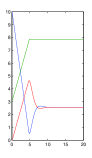
(a) Clustering

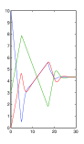
(b) Consensus

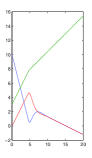
(c) Unstable

Figure 3: The trajectories of the storage at the vertices

Now let us consider the closed-loop system (19) defined on a general graph. At this moment we will only give a sufficient condition for the system (19) under arbitrary constraints to reach load balancing (consensus). Consider a strongly connected network compatible with the constraint intervals $[u^{-},u^{+}]$. According to Lemma 4, suppose there exists $k$ cycles to cover the graph, denoted as $\mathcal{T}=(C_{1},C_{2},\ldots,C_{k})$. Given $\mathcal{T}$, we can define a multiplicity vector $T\in\mathbb{R}^{m}$ whose $i$-th component is the number of cycles in $\mathcal{T}$ which contain the $i$-th edge. Then we construct an augmented network $\tilde{\mathcal{G}}(\mathcal{T})$ by splitting each edge of $\mathcal{G}$ into multiple edges based on their multiplicities, using the identity (20). For instance, if the $i$-th edge of $\mathcal{G}$ has been used $T_{i}$ times in $\mathcal{T}$ then we splitting $i$-th edge into $T_{i}$ edges. The newly generated edges have constraint intervals $[u^{-}_{i},b_{2}],[0,b_{3}-b_{2}],\ldots,[0,u^{+}_{i}-b_{T_{i}}],$ for arbitrary $u^{-}_{i}<b_{2}<\cdots<b_{T_{i}}<u^{+}_{i}$. Furthermore, it can be easily seen that $\tilde{\mathcal{G}}(\mathcal{T})$ is balanced, and that it can be covered by non-overlapping cycles. We denote the set of cycles to cover $\tilde{\mathcal{G}}(\mathcal{T})$ by $\tilde{\mathcal{T}}$. The above process can be explained by the following example.

Example V.4

In this example, we consider the graph $\mathcal{G}$ given as in Figure. 4(left). Notice that $\mathcal{G}$ is unbalanced and that $\mathcal{T}=\{C_{1},C_{2}\}$ is a minimal covering set where $C_{1}=\{e_{1},e_{2},e_{3}\}$ and $C_{1}=\{e_{3},e_{4},e_{5}\}$. So the corresponding multiplicity vector $T$ is given as $T=[1,1,2,1,1]^{T}.$

By dividing $e_{3}$ into two edges, we obtain the augmented graph $\tilde{\mathcal{G}}(\mathcal{T})$ as in Figure.4(right). Here the constraint intervals for the edge $e_{3_{1}}$ and the edge $e_{3_{2}}$ in $\tilde{\mathcal{G}}(\mathcal{T})$ are $[u^{-}_{3},b],[0,u^{+}_{3}-b]$ respectively, while $[u^{-}_{3},u^{+}_{3}]$ is the constraint interval for $e_{3}$ in $\mathcal{G}$ with $u^{-}_{3}<b<u^{+}_{3}$.

Now $\tilde{\mathcal{G}}(\mathcal{T})$ is balanced and can be covered by non-overlapping cycles. Indeed, $\tilde{\mathcal{T}}=\{\tilde{C}_{1},\tilde{C}_{2}\}$ where $\tilde{C}_{1}=\{e_{1},e_{2},e_{3_{1}}\}$ and $\tilde{C}_{2}=\{e_{4},e_{5},e_{3_{2}}\}.$

Figure 4: Left: The graph $\mathcal{G}$. Right: The augmented graph $\tilde{\mathcal{G}}(\mathcal{T})$.The generation of the augmented graph $\tilde{\mathcal{G}}(\mathcal{T})$ based on $\mathcal{T}$.

The main result of the paper can be summarized as the following theorem substantially generalizing Lemma 5.

Theorem 8

Consider the closed-loop dynamical system (19) defined on a strongly connected graph which is compatible with the constraint intervals. Let $\mathcal{T}$ be a minimal covering set for $\mathcal{G}$ and let $\tilde{\mathcal{G}}(\mathcal{T})$ be the augmented graph based on $\mathcal{T}$. Let $\tilde{\mathcal{T}}=(\tilde{C}_{1},\tilde{C}_{2},\ldots,\tilde{C}_{k})$ be a covering set of cycles for $\tilde{\mathcal{G}}(\mathcal{T})$. If there exists a splitting of the overlapped edges in $\mathcal{G}$ such that the intersection of all constraint intervals of each cycle $\tilde{C}_{i},i=1,2,\ldots,k$ has non-empty interior, then the trajectories of the system (19) will converge to

$$\mathcal{E}_{\mathrm{tot}}= \{(x,x_{c})\mid\frac{\partial H}{\partial x}(x)=\alpha\mathds{1},\,\alpha\in\mathbb{R},\,$$ (36)

$$B\operatorname{sat}(-x_{c}\,;u^{-},u^{+})=0\,\}.$$

Proof:

Because of lack of space, we only give a sketch of the proof. Consider the same Lyapunov function (28). If we choose a constant vector $(\nu,x_{c}(0))\in\mathcal{I}$, which is the largest invariant set in $\{(x,x_{c})\mid\dot{V}=0\}$, then along this trajectory $V(\nu,B^{T}\frac{\partial H}{\partial x}(\nu)t+x_{c}(0))$ is constant for all time $t\geqslant 0$. Suppose $B^{T}\frac{\partial H}{\partial x}(\nu)\neq 0$, then by the fact that $\tilde{\mathcal{G}}(\mathcal{T})$ can be covered by non-overlapping cycles, we can prove that for $t$ large enough, $\frac{d}{dt}V(\nu,B^{T}\frac{\partial H}{\partial x}(\nu)t+x_{c}(0))>0$. This yields a contradiction. ∎

Example V.5

The sufficiency condition in Theorem 8 is not a necessary condition. Indeed, consider the dynamic (19) defined on the network given in Fig.4(left). The constraint intervals for $e_{i},i=1,2,\ldots,5$ are $[0.3,1]$, $[0.3,1]$, $[0.5,0.8]$, $[0.3,1]$, $[0.3,1]$ respectively. There does not exist any splitting such that the intersections of the constraint intervals have nonempty interior. However $\frac{\partial H}{\partial x}(x(t))$ converges to consensus. A special case with $H(x)=\frac{1}{2}\|x\|^{2}$ is shown in Fig.5.

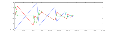
Figure 5: The trajectories of the storage at the vertices

VI CONCLUSIONS

We have discussed a basic model of dynamical distribution networks where the flows through the edges are generated by distributed PI controllers. The resulting system can be naturally modeled as a port-Hamiltonian system with arbitrary flow constraint intervals. Key tools in the analysis are the construction of a $C^{1}$ Lyapunov function and the observation given in Lemma 4. Based on that, we have derived necessary and sufficient conditions for asymptotic consensus and clustering for a dynamical system defined on a cycle. For arbitrary networks we have obtained a sufficient condition for consensus or clustering.

An obvious open problem is to find sufficient and necessary conditions for an arbitrary network to reach consensus or clustering. This is currently under investigation. Many other questions can be addressed within the same framework. For example, what is happening if the in/outflows are not assumed to be constant, but are e.g. periodic functions of time; see already [14].

References

- [1] A.J. van der Schaft and J. Wei, “A hamiltonian perspective on the control of dynamical distribution networks,” 4th IFAC Workshop on Lagrangian and Hamiltonian Methods for Non Linear Control, pp. 24–29, 2012.
- [2] A.J. van der Schaft and B.M. Maschke, “Port-Hamiltonian systems on graphs,” SIAM J. Control and Optimization, vol. 51(2), pp. 906–937, 2013.
- [3] A.J. van der Schaft and B.M. Maschke, “Conservation laws on higher-dimensional networks,” Proc. 47th IEEE Conf. on Decision and Control, 2008.
- [4] ——, Model-Based Control: Bridging Rigorous Theory and Advanced Technology, P.M.J. Van den Hof, C. Scherer, P.S.C. Heuberger, eds., chapter Conservation laws and lumped system dynamics. Berlin-Heidelberg: Springer, 2009.
- [5] ——, “Port-Hamiltonian dynamics on graphs: Consensus and coordination control algorithms,” Proc. 2nd IFAC Workshop on Distributed Estimation and Control in Networked Systems, pp. 175–178, 2010.
- [6] M. Bürger and D. Zelazo and F. Allgöwer, “Network clustering: A dynamical systems and saddle-point perspective,” IEEE Conference on Decision and Control, pp. 7825–7830, 2011.
- [7] D. Zelazo and M. Mesbahi, “Edge agreement: Graph-theoretic performance bounds and passivity analysis,” Automatic Control, IEEE Transactions on, vol. 56, no. 3, pp. 544 –555, march 2011.
- [8] F. Blanchini, S.Miani, and W.Ukovich, “Control of production-distribution systems with unknown inputs and system failures,” Automatic Control, IEEE Transactions on, vol. 45, no. 6, pp. 1072–1081, 2000.
- [9] D.Bauso, F.Blanchini, L.Giarré, and R.Pesenti., “A decentralized solution for the constrained minimum-norm flow,” Submitted to Automatic Control, IEEE Transactions on, 2011.
- [10] J. Wei and A.J. van der Schaft, “Load balancing of dynamical distribution networks with flow constraints and unknown in/outflows,” Accepted by Systems & Control Letters, 2013.
- [11] B. Bollobas, Modern Graph Theory, ser. Graduate Texts in Mathematics. New York: Springer, 1998, vol. 184.
- [12] A.J van der Schaft and B.M. Maschke, “The Hamiltonian formulation of energy conserving physical systems with external ports,” Archiv für Elektronik und Übertragungstechnik, vol. 49, pp. 362–371, 1995.
- [13] A.J. van der Schaft, -Gain and Passivity Techniques in Nonlinear Control, ser. Lect. Notes in Control and Information Sciences. Berlin: Springer-Verlag, 1996, vol. 218.
- [14] C. D. Persis, “Balancing time-varying demand-supply in distribution networks: an internal model approach,” arxiv, 2013.