Spinning black hole in the puncture method: Numerical experiments

Abstract

The strong-field region inside a black hole needs special attention during numerical simulation. One approach for handling the problem is the moving puncture method, which has become an important tool in numerical relativity since it allows long term simulations of binary black holes. An essential component of this method is the choice of the ’1+log’-slicing condition. We present an investigation of this slicing condition in rotating black hole spacetimes. We discuss how the results of the stationary Schwarzschild ’1+log’-trumpet change when spin is added. This modification enables a simple and cheap algorithm for determining the spin of a non-moving black hole for this particular slicing condition. Applicability of the algorithm is verified in simulations of single black hole, binary neutron star and mixed binary simulations.

1 Introduction

The moving puncture method is a successful approach for the simulation of black holes, see [1, 2] for pedagogic explanations and references. Numerically the method can be applied to multiple, spinning black holes in quasi-circular or eccentric orbits, but analytical results are only known for the Schwarzschild spacetime. Without spin and linear momentum a single black hole settles down to a stationary state similar to a ’trumpet’, containing one asymptotically flat end and one with finite Schwarzschild radius, e.g. [3, 4, 5, 6]. In this article we begin an investigation of punctures in axisymmetry by performing numerical experiments of rotating black holes. We will show that the spinning puncture settles down to a stationary state similar to the spherical symmetric case and generalize results obtained for the Schwarzschild spacetime. A short description about possible modification of the ansatzes of [3] will be given, which offers the possibility to read off the spin value directly without additional computational costs.

2 Spinning Puncture

2.1 Numerical setup

We use the BAM-code [7] for fully general relativistic evolutions with the moving puncture method [8, 9]. Unless otherwise stated the total mass of the system $M$ is set to unity and the spin axis is equivalent to the z-axis. We use the BSSN [10, 11] evolution scheme for the numerical evolution. As a particular gauge choice, we apply the commonly used 1+log-slicing condition [12] together with the $\tilde{\Gamma}$-driver shift [13]. This special choice, sometimes called moving puncture coordinates, is well established in numerical relativity and widely used.

2.2 Stationarity

As a starting point, we want to demonstrate that for spinning punctures a stationary state is reached similar to the one in spherical symmetry. For this purpose, we consider the trace of the extrinsic curvature $K$ as a function of the lapse $\alpha$, because $K(\alpha)$ is independent of the spatial coordinates as long as we use the same slicing condition for all simulations. When a stationary state is reached, the difference of $K(\alpha)$ between two hypersurfaces, i.e. $||\Delta K(\alpha)||_{2}=\sqrt{\int|K(\alpha)_{t_{1}}-K(\alpha)_{t_{2}}|^{2}},$ becomes zero for $t\rightarrow\infty$. In Fig. 2 we compare directly the spinning and the non-spinning configuration. We know that the non-spinning puncture reaches a stationary state and the same seems to be true for the spinning black hole. Additionally, one can show that the time derivatives of the evolution variables become zero. We checked this for the lapse $\alpha$ by computing the right hand side of the 1+log-slicing condition, e.g. for a black hole with $j=0.4$ the derivative after $100M$ is smaller than $5\cdot 10^{-5}$.

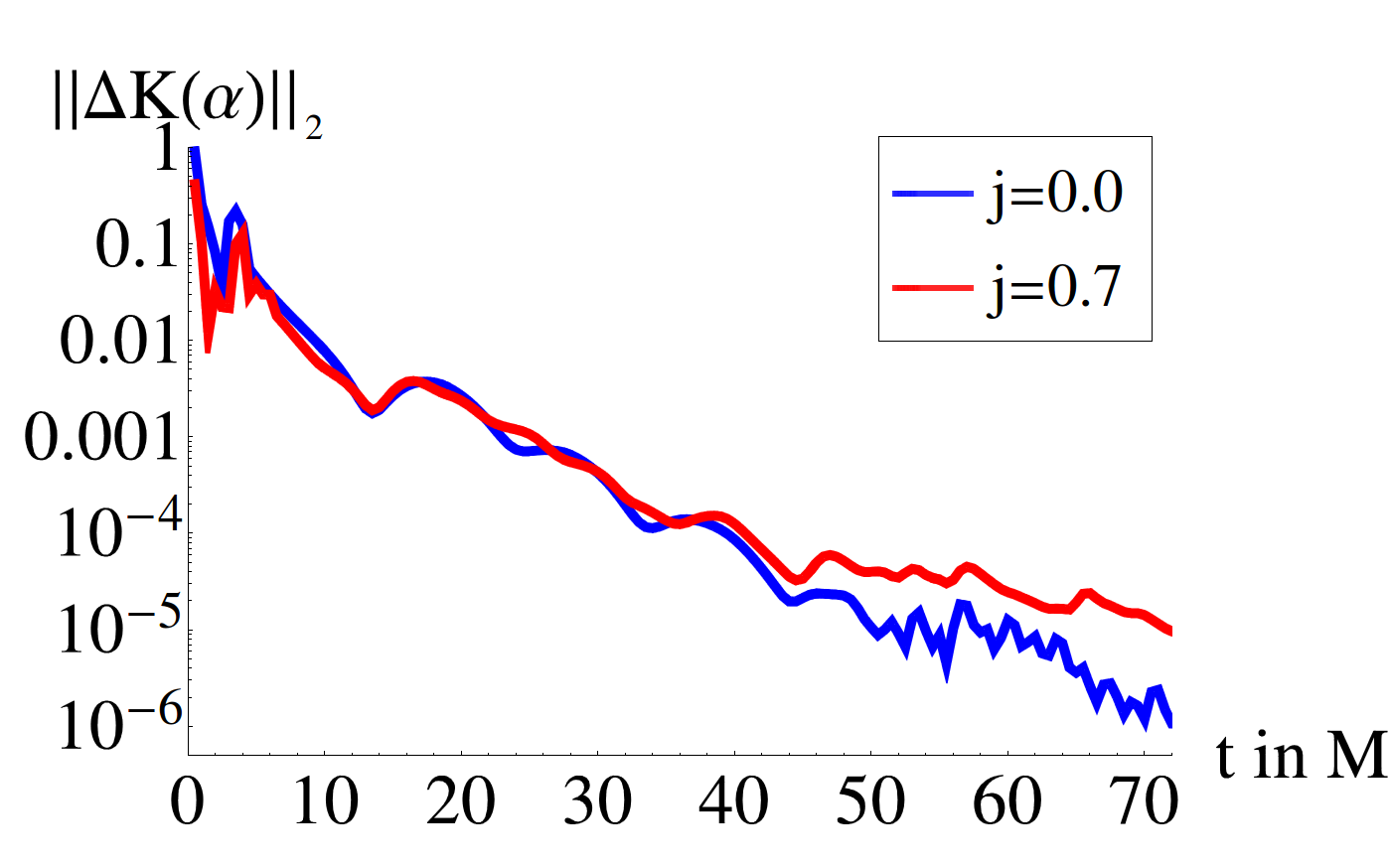
Figure 1: $||\Delta K(\alpha)||_{2}$ for $j=0.0$ and $j=0.7$ with $t_{1}-t_{2}=0.5M$.

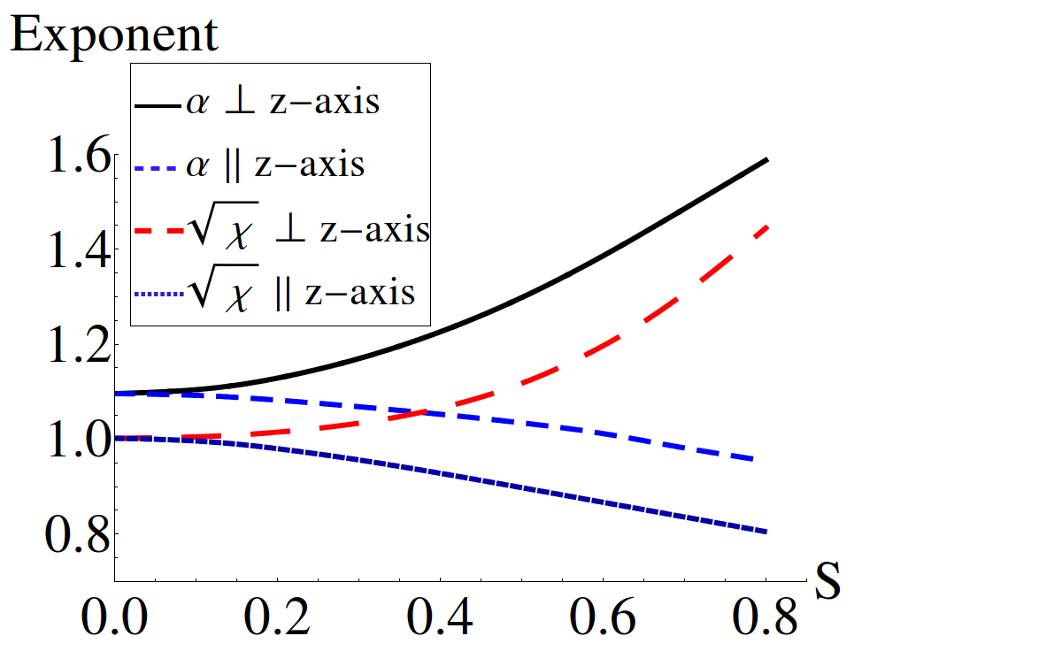
Figure 2: Exponents for the lapse and the conformal factor along different axes.

2.3 Influences on the BSSN-evolution variables

The stationary state in spherical symmetry can be computed semi-analytically. The lapse behaves near the puncture like $\alpha\sim r^{1.0916}$, see [6]. We find an exponent of $\gamma=1.091$ when we use our numerical data and apply the fitting function $\alpha=\alpha_{0}+\alpha_{1}r^{\gamma}(1+\alpha_{2}r+\alpha_{3}r^{2})$. We can do the same for the conformal factor $\psi$ and get for $\sqrt{\chi}=\psi^{-2}$ with $\sqrt{\chi}=c_{0}+c_{1}r^{\gamma}(1+c_{2}r+c_{3}r^{2})$ an exponent of $\gamma=1.002$, while $\gamma=1.000$ is the analytical result. One should mention that we are using the radial coordinate of our numerical grid $r$, which does not necessarily agree with the isotropic radius for which the exponents were derived in [6], but because of the particular gauge choices both descriptions become approximately the same near the puncture. Thus, we will use the coordinate radius to get a better insight in the numerical simulation, not necessarily in the geometry of the spacetime. According to Fig. 2 the exponents of $\alpha$ and $\sqrt{\chi}$ change differently, depending on the axis between the spin and the axis used for the fit.

Remarkable is that even when the exponent is decreasing the puncture method works and can handle the non-differentiable functions. The important point is that although the regularity of the functions is reduced, compared with spherical symmetry, the moving puncture method does not fail. This effect could explain why stationary spinning punctures are less accurate than non-spinning punctures in numerical simulations [14]. Additionally, the angular dependence of the exponent $\gamma$ complicates possible attempts to factor out the singularity analytically.

Independent of the non-integer powers of $r$ for $\alpha$ and $\sqrt{\chi}$, we can use a Taylor expansion to model the behavior near the black hole, see [3] for the description in spherical symmetry. Considering axisymmetry we have to introduce an additional angular dependence, where we define $\varphi$ as the angle between the axis of rotation $S^{i}$ and $n^{i}$ as the outward-pointing unit radial vector. This dependence is described reasonably well with spherical harmonics, e.g. for the trace of the extrinsic curvature $K=\sum_{i=0}^{\infty}K_{i}r^{i}$, where we choose $K_{i}=\sum_{l=0}^{\infty}K_{il}Y_{2l,0}(\varphi,0)$ to encode axisymmetry in the components $K_{i}$. The same holds for the other BSSN scalars. The shift vector $\beta^{i}$ in axial symmetry can be described by $\beta^{i}=(b_{1}r+b_{2}r^{2})n^{i}+(c_{1}r+c_{2}r^{2})\bar{\epsilon}^{ijk}n_{j}S_{k},$ where we introduced the additional term $(c_{1}r+c_{2}r^{2})\bar{\epsilon}^{ijk}n_{j}S_{k}$. A closed description of the extrinsic curvature $\tilde{A}_{ij}$ and the conformal metric $\tilde{g}_{ij}$ is more complicated and is explained up to some point in [15].

3 Spin-determination without integration

3.1 The new algorithm

An important issue during the numerical evolution of black holes is obtaining a good estimate of the black hole spin. Using the properties of the stationary state described in sec. 2.2, it is simple to find the spin of a non-moving black hole evolved with the puncture gauge. For increasing spin the absolute value of $K$ at the puncture, $K_{0}$, becomes smaller. The behavior is well approximated by a quadratic function. Inverting this formula leads to

$$S=\sqrt{1.41789-4.71218K_{0}},$$ (1)

which correlates an evolution variable of the BSSN scheme and properties of the underlying spacetime. Thus, we are able to read off the amplitude of the spin of a non-moving puncture simply by measuring $K_{0}$. To get the entire information of the black hole spin we need the spin axis. This can be found with the lapse $\alpha$. Our experiments showed that the coordinate distance between the origin and a contour line is smallest when we look along the rotation axis, see Fig. 3. The direction of rotation can be determined with the shift vector $\beta^{i}$, because of the additional term $(c_{1}r+c_{2}r^{2})\bar{\epsilon}^{ijk}n_{j}S_{k}$. Empirical studies showed $c_{1}>0$, so we can find the sign of $S_{k}$ by regarding $\beta^{i}$ along one axis.

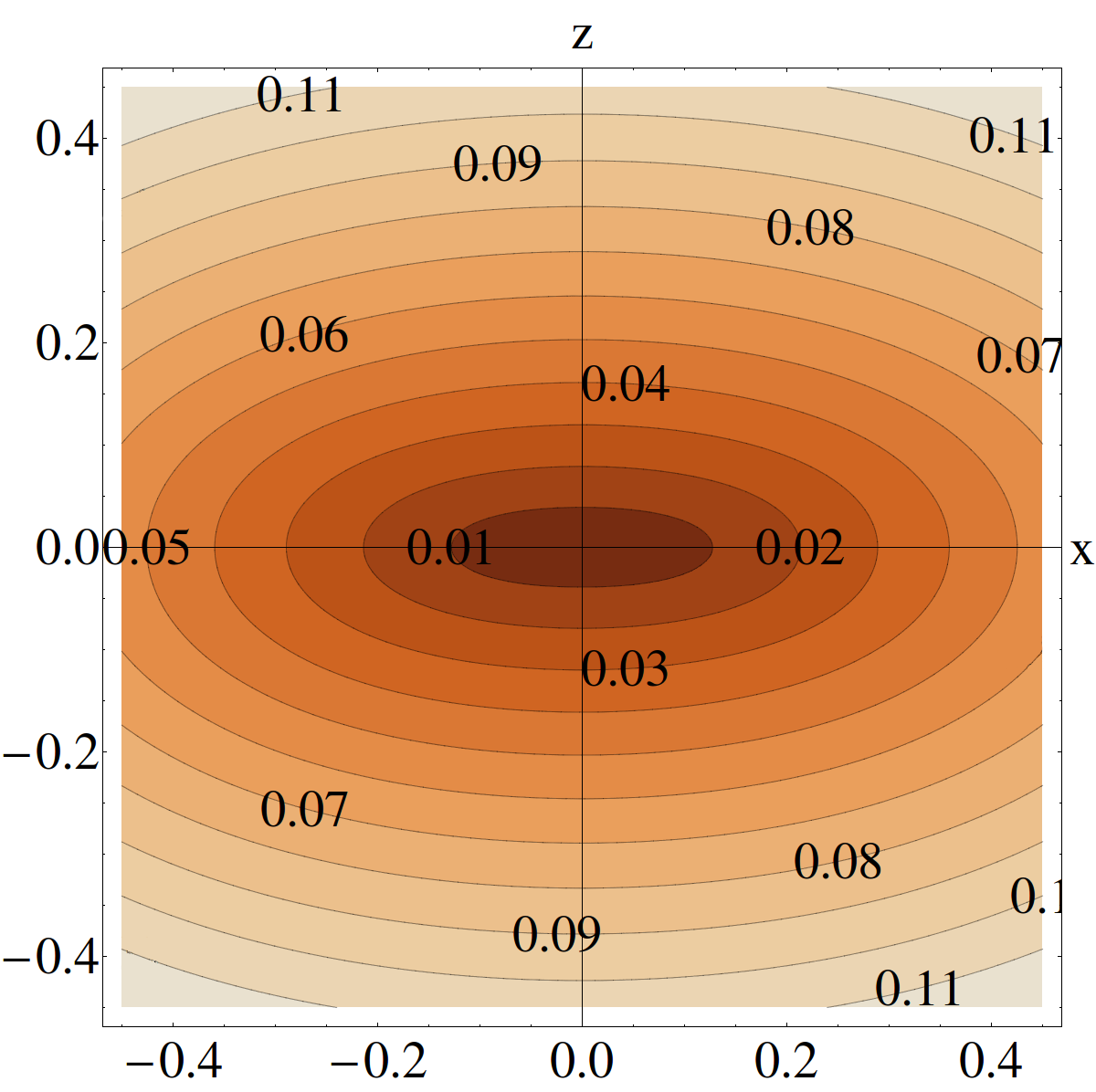
Figure 3: Level surface of $\alpha$ for a black hole with $j=0.8$. Although the contour lines might suggest that the puncture is stretched to a one dimensional line instead of a single point numerical experiments showed no indication that the puncture has an extension $>10^{-3}M$. Thus, also a spinning puncture can be treated as a point.

3.2 Numerical tests and measurement uncertainties

The first test for the validity of our new algorithm are single black hole simulations. Table 1 shows some test cases in which the spin was calculated using BAM’s curvature flow apparent horizon finder and the new method. For further tests we include results for the final remnant of a mixed binary (BHNS) and a neutron star binary (NSNS) merger. Comparing with the apparent horizon finder, the results agree within the estimated uncertainty.

To define the measurement uncertainty we investigate every part of our algorithm individually. The first step is to determine the absolute spin value with the help of the interpolation function (1). The error comes from the estimate of $K_{0}$ and can be evaluated by using different resolutions. Using the corresponding uncertainty, we can compute the error according to equation (1), including also the standard error of the regression. The second step of our algorithm defines the angular uncertainty. Considering a box with $N^{3}$ grid points the angular error is approximately $2/N$, in our case $\lesssim 0.02rad$. On the other hand using an interpolation to find the level surface one achieves a much lower uncertainty of around $\sim 10^{-3}rad$. Because the last step of our algorithm uses only the qualitative behavior of $\beta^{i}$, it comes without an additional error. We can sum up that our method determines the spin with an uncertainty of $\Delta S\lesssim 0.02$ and an angular resolution of at least $0.02rad$ for $j\gtrsim 0.2$. For smaller spins the change of $S(K)$ in equation (1) is small, which leads to higher uncertainties. Furthermore, equation (1) was defined as an adequate function for $j\in[0,0.7]$, nevertheless using higher resolution for higher spins the method is applicable as well.

Table 1: Single black hole simulations (left) and results for the final remnant for a binary merger (right). The first line refers to the new algorithm, the second line to the apparent horizon finder.

BH-mass $S_{x}$ $S_{y}$ $S_{z}$ j 1 0.10 0.66 0.21 0.70$\pm$0.01 0.11 0.66 0.20 0.70 1 0.09 -0.50 0.21 0.55$\pm$0.01 0.10 -0.50 0.20 0.55 1.92 0.04 -0.32 0.15 0.10$\pm$0.07 0.10 -0.50 0.20 0.15 system $M_{ADM}^{init}$ $K_{0}$ $j$ BHNS $8.328M_{\astrosun}$ $\sim 0.0315M_{\astrosun}$ $0.42\pm 0.05$ $0.43$ NSNS $2.998M_{\astrosun}$ $\sim 0.059M_{\astrosun}$ $0.76\pm 0.04$ $0.76$ NSNS $3.439M_{\astrosun}$ $\sim 0.057M_{\astrosun}$ $0.71\pm 0.05$ $0.70$

4 Conclusion

We presented numerical results for rotating black holes and generalized the ansatzes of [3]. For spinning punctures a simple $r^{\gamma(\varphi)}$-model for the evolution variables is possible, where in contrast to spherical symmetry the exponent depends on the angle $\varphi$. This complicates attempts to factor out the singularity analytically. In the future we plan to use these results to find an analytical description for a rotating black hole using the moving puncture gauge.

Additionally, a fast algorithm was introduced to determine the spin of a non-moving puncture. Adding linear momentum to a spinning black hole to obtain a binary orbit breaks the axisymmetry, but a generalization of the numerical method appears possible.

References

References

- [1] Alcubierre M 2008 Introduction to 3+1 Numerical Relativity (Oxford University Press)
- [2] Baumgarte T and Shapiro S 2010 Numerical Relativity: Solving Einsteins Equations on the Computer (Cambridge University Press)
- [3] Hannam M, Husa S, Pollney D, Brügmann B and Ó Murchadha N 2007, Phys. Rev. Lett. 99 241102
- [4] Brown J 2008 Phys. Rev. D 77 044018
- [5] Hannam M, Husa S, Ohme F and Ó Murchadha N 2008 Phys. Rev. D 78 064020
- [6] Brügmann B 2009 Gen. Rel. Grav. 41 p.2131-51
- [7] Brügmann B, Gonzales J, Hannam M, Husa S, Sperhake U and Tichy W 2008 Phys. Rev. D 77 024027
- [8] Campanelli M, Lousto C O, Marronetti P and Zlochower Y 2006 Phys. Rev. Lett. 96 111101
- [9] Baker J G, Centrella J, Choi D I, Koppitz M and van Meter J 2006 Phys. Rev. D 73 104002
- [10] Shibata M and Nakamura T 1995 Phys. Rev. D 52 p. 5428-44
- [11] Baumgarte T and Shapiro S 1998 Phys. Rev. D 59 024007
- [12] Bona C, Seidel E and Stela J 1995, Phys. Rev. Lett. 75 p. 600-603
- [13] Alcubierre M, Brügmann B, Diener P, Koppitz M, Pollney D, Seidel E and Takahashi R 2003, Phys. Rev. D 67 084023
- [14] Lousto C and Zlochower Y 2009 Phys. Rev. D 79 064018
- [15] Dietrich T 2012 Black Hole Data in Axial symmetry, Master Thesis at University of Jena