Generation of uniform synthetic magnetic fields by split driving of an optical lattice

Abstract

We describe a method to generate a synthetic gauge potential for ultracold atoms held in an optical lattice. Our approach uses a time-periodic driving potential based on quickly alternating two Hamiltonians to engineer the appropriate Aharonov-Bohm phases, and permits the simulation of a uniform tunable magnetic field. We explicitly demonstrate that our split-driving scheme reproduces the behavior of a charged quantum particle in a magnetic field over the complete range of field strengths, and obtain the Hofstadter butterfly band-structure for the Floquet quasienergies.

Introduction – Systems of ultracold atoms held in optical lattice potentials have an exceptionally high degree of controllability and excellent coherence properties. As such they have proven to be excellent systems for simulating bloch_sim Hamiltonians arising in diverse areas of physics, such as graphene wuns08 ; graphene , Majorana fermions majorana , and models of high-temperature superconductivity hubbard . A topic of intense current activity is how to reproduce the effects of gauge fields in these systems. This would not only extend the use of cold-atom simulators to new domains, but is also of considerable interest to applications such as quantum computation. A particularly important example is the $U(1)$ gauge of electromagnetism. The ability to simulate magnetic fields would give exciting new ways to explore quantum Hall physics and related effects such as topological insulators and anyon physics, together with the realization of phenomena such as the Hofstadter butterfly hofstadter , a fractal energy spectrum seen in lattice systems exposed to high magnetic fluxes.

Many efforts to simulate an applied magnetic field with cold atoms have used laser-driven transitions between internal atomic states to generate phases raman ; jaksch ; lewenstein which mimic the Aharonov-Bohm phases that would be experienced by charged particles moving in a uniform magnetic field. An attractive alternative to these schemes is to use inertial forces, which do not require a specific internal state structure, and so are applicable to a wider range of atomic species. First efforts of this kind coriolis used rotation to generate a Coriolis force, which has an analogous form to the Lorentz force of electromagnetism. Only weak fields, however, were accessible by this method.

An alternative inertial approach is to periodically accelerate (or “shake”) the lattice to produce the effect known as coherent destruction of tunneling, a quantum coherent effect in which the driving renormalizes the tunneling amplitude CDT . This effect has been directly observed in the expansion dynamics of atomic clouds arimondo_J0 ; arimondo_Jn ; cec_morsch . More recently, it has also been noted that the driving can be used to render the tunneling complex cec_J0 ; cec_phase ; longhi , giving the prospect of generating synthetic magnetic fields. This possibility has been explored experimentally first in one-dimensional lattices eckardt1 , and later in a triangular lattice where this effect was used to create a staggered field eckardt2 .

Generating a uniform field on a square lattice, however, is not straightforward, and an initial proposal kolovsky was later found to contain a problem that limited it to only inhomogeneous fields comment . Very recently experimental progress has been made ketterle ; bloch by introducing additional lattice potentials and a strong magnetic field gradient. In this work we address the problem in a different way by borrowing the well-known split-operator technique from quantum simulation to develop an alternative method that we term “split driving”. This consists of dividing the time-dependent Hamiltonian into two parts, namely tunneling in the $x$ and $y$ directions, and applying the parts sequentially. We show that this avoids the problems encountered previously kolovsky , and indeed makes it possible to simulate a practically uniform synthetic field of arbitrary strength using only the manipulation of the time-dependent driving potential, without requiring the complication of external magnetic fields. Furthermore, as our scheme can work with small driving amplitudes, heating effects can be minimal ketterle , enhancing the chance to observe the Hofstadter butterfly troyer .

Method – To illustrate the main ideas we schematically show a possible arrangement in Fig.1a. We consider a two-dimensional optical lattice, formed by the superposition of two orthogonal standing waves. When the optical lattice is sufficiently deep, a system of cold atoms can be described well by a tight-binding (hopping) Hamiltonian

$$H(t)=-J\sum_{i}\left(a_{i}^{\dagger}a_{i+{\hat{x}}}+a_{i}^{\dagger}a_{i+{\hat{y}}}+\mathrm{H.c.}\right)+H_{I}(t)$$ (1)

where $J$ is the hopping between nearest-neighbors and $a_{i}\ /a_{i}^{\dagger}$ are the standard particle annihilation/creation operators for lattice site $i$. Acceleration of the lattice in the $x$-direction can be viewed in the rest frame of the lattice as arising from an inertial force, described as a scalar potential depending linearly on $x$, $H_{I}(t)=V(t)\sum_{j}x_{j}n_{j}$ where $x_{j}$ is the $x$-coordinate of lattice-site $j$ and $n_{j}$ is the number operator. We take the specific form for the driving

$$V(t)=V_{0}+K\cos\left(\omega t+\alpha\right)\ ,$$ (2)

consisting of a constant and an oscillation, parameterized by $V_{0}$ and $K$ respectively. The frequency of the oscillation is $\omega$, and $\alpha$ is the driving phase-shift which will play an important role. The driving starts at $t=0$. We assume that the resulting discontinuity at $V(t=0)$ is experimentally feasible, due to the relatively slow dynamics of cold atoms.

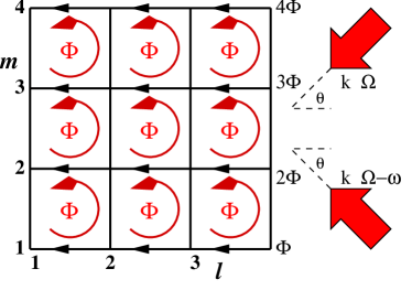
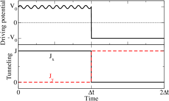
Figure 1: (a) Schematic representation of the method. The optical lattice is formed as a two-dimensional standing wave between incoming laser beams, and is periodically accelerated in the $x$ direction, producing an inertial force in the lattice rest-frame. Two additional running-wave beams, with a frequency difference $\omega$ and crossing at an angle of $2\theta$, add a spatially-dependent phase to the driving. In the Landau gauge the tunneling phases $\chi$ appear only on the horizontal hopping processes (marked with arrows). A linear variation of the phase with $y$, $\chi(m)=m\Phi$, would produce a uniform flux $\Phi$ threading each plaquette. (b) The split-driving scheme. In the first half-period, an acceleration consisting of a constant and oscillating component is applied in the $x$-direction (upper figure) to induce the Aharonov-Bohm tunneling phases, while the tunneling in the $y$ direction ($J_{y}$) is suppressed (lower figure). In the second half-period the $x$-coordinate is uniformly accelerated back to its original position, suppressing the $x$-tunneling ($J_{x}$) via the Wannier-Stark effect, while tunneling in the $y$ direction is restored. This pattern of driving is periodically repeated.

We begin by considering the simplest case of constant $\alpha$, and throughout this work we shall work with resonant driving, $V_{0}=n\omega$ where $n$ is an integer, and we take $\hbar=1$. In the limit of high frequencies, $\omega\gg J$, the system can be described by an effective static hopping Hamiltonian, with an effective $x$-hopping given by cec_phase

$$J_{\mathrm{eff}}=J\ e^{i\left(K/\omega\right)\sin\alpha}\ e^{in\left(\alpha+\pi\right)}\ {\cal J}_{n}\left(K/\omega\right),$$ (3)

for right-to-left hopping, and $J_{\mathrm{eff}}^{\ast}$ for left-to-right movement. Note that for $\alpha=0$ this reduces to the well-known Bessel function renormalization holthaus_Jn , $J_{\mathrm{eff}}=(-1)^{n}J{\cal J}_{n}\left(K/\omega\right)$. From Eq. (3) we can clearly see that the driving in general produces a tunneling-phase cec_phase , $\chi=\left(K/\omega\right)\sin\alpha+n(\alpha+\pi)$. For one-dimensional systems this has been proposed as a means to induce transport cec_phase ; cec_J0 , and the effects of $\chi$ have been experimentally observed in experiments on driven “super-Bloch oscillations” innsbruck ; tania_phase .

The magnetic flux passing through a plaquette is evaluated by summing the complex phases acquired on each tunneling process as the plaquette is traversed anti-clockwise. Clearly when $\chi$ is constant the flux is zero footnote_phase , and so to produce a synthetic flux $\chi$ must vary in space. The specific case of the Landau gauge $\chi(m)=m\Phi$, where $m$ indexes the $y$-coordinate, is shown in Fig.1a, which results in every plaquette being threaded by a net flux $\Phi$. To mimic this gauge we therefore make the phase-shift similarly spatially-dependent, $\alpha\rightarrow\alpha(m)=m\phi$. From Eq. (3) this gives an effective flux per plaquette of

$$\Phi(m)=n\phi+\left(K/\omega\right)\left[\sin\left(\left(m+1\right)\phi\right)\ -\ \sin\left(m\phi\right)\right]\ .$$ (4)

The first term of this expression indeed reproduces the Landau gauge of a uniform synthetic flux, while the second corresponds to a flux that varies with $y$. Its value, however, is bounded, $|\Phi_{\mathrm{var}}|\leq 2\left|\left(K/\omega\right)\sin\left(\phi/2\right)\right|$, and so can be controlled by setting $K/\omega$ sufficiently small. Besides generating an essentially uniform $\Phi$, making $K/\omega$ small has the additional advantage of limiting lattice heating effects, although as this reduces the amplitude of $J_{\mathrm{eff}}$ this also has the effect of slowing the system’s dynamics.

In an experimental realization, we thus need to introduce two vital ingredients; a time-dependent driving potential to produce photon-assisted tunneling in the $x$ direction, and a $y$-dependence of the phase, $\alpha(m)$, that is imprinted on this tunneling. This can be done in a number of different ways, and in the particular scheme shown in Fig. 1a it is produced by a pair of far-detuned running wave beams with wavevector $k$ and a frequency difference of $\omega$ between them. This produces a time-dependent optical potential $V_{\mathrm{RW}}(x)\cos^{2}\left(\omega t/2+ky\sin\theta\right)$, where $2\theta$ is the angle between the beams and $V_{\mathrm{RW}}(x)$ is the envelope function of the light intensity. If this varies weakly with $x$ then to first order we can write kolovsky

$$V_{\mathrm{RW}}(x)\simeq V_{\mathrm{RW}}(0)+x\frac{\partial V_{\mathrm{RW}}}{\partial x}\ ,$$ (5)

where the first term is an unimportant constant, and the second produces the oscillatory component of the driving potential. In combination with a uniform acceleration of the optical lattice, this gives a potential which is a generalization of Eq.2 in which the phase, $\alpha$, varies with position

$$V(m,t)=V_{0}+K\cos\left(\omega t+\alpha(m)\right)\ ,$$ (6)

where $\alpha(m)=2kd_{L}m\sin\theta$ and $d_{L}$ is the optical lattice spacing (henceforth we take $d_{L}=1$), and $K=V^{\prime}_{\mathrm{RW}}/2$. In practice the gradient $V^{\prime}_{\mathrm{RW}}$ does not have to be strictly constant over the entire cloud, as long as its variation is sufficiently weak that Eq. 5 is valid. Interference between the optical lattice and the running-wave beams can be avoided by using acoustic-optic modulators to produce frequency offsets, as described in Ref.ketterle . Unfortunately, when $\alpha(m)$ varies in this way, the potential (6) has the undesired effect of also driving tunneling in the $y$-direction since the potential difference between a site and its neighbors in the $y$-direction, $V(m\pm 1,t)-V(m,t)$, is in general a time-dependent quantity, oscillating with frequency $\omega$ comment .

To eliminate this unwanted renormalization of the $y$-tunneling, we apply the split-operator technique soren familiar from numerical studies of quantum systems, and divide the time-evolution operator over a short time-interval into two parts, as shown in Fig. 1b. In the first interval the lattice is driven by the potential (6), while the $y$-hopping is suppressed (for example, by increasing the depth of the optical lattice in the $y$-direction). In this interval $H(t)$ can thus be replaced by an effective static Hamiltonian, $H_{x}^{\mathrm{eff}}$, which contains only $x$-hopping terms in which the tunneling has been renormalized. In the second interval we restore the $y$-hopping, and instead suppress the $x$-hopping, so that the system evolves under $H_{y}$, a time-independent Hamiltonian containing only the $y$-hopping operators. A convenient way to do this is to flip the sign of the acceleration of the lattice ($V_{0}\rightarrow-V_{0}$ while setting $K=0$) so that the intersite tunneling in the $x$-direction is destroyed by Wannier-Stark localization. This has the additional practical benefit of keeping the average displacement of the lattice zero footnote , otherwise the constant acceleration would quickly move the lattice out of the experimental area.

This division amounts to a Suzuki-Trotter decomposition of $H(t)$

$$e^{-i\left(H_{x}^{\mathrm{eff}}+H_{y}\right)\Delta t}\simeq e^{-iH_{x}^{\mathrm{eff}}\Delta t}e^{-iH_{y}\Delta t}\ .$$ (7)

As $H_{x}^{\mathrm{eff}}$ and $H_{y}$ do not commute, the leading error in this decomposition is given by the Baker-Campbell-Hausdorff formula $\frac{\Delta t^{2}}{2}\left[H_{x}^{\mathrm{eff}},H_{y}\right]\sim JJ_{\mathrm{eff}}\Delta t^{2}$. More complicated decompositions can be used in which the error term decays more rapidly suzuki , but for simplicity we limit ourselves to the most primitive form. Henceforth we set the tunneling in the $y$ direction $J_{y}=J_{\mathrm{eff}}$, so that the error terms arising in the two time intervals, $(J\Delta t)$ and $(J_{\mathrm{eff}}\Delta t)$ are equal. If $J_{\mathrm{eff}}\neq J$ the same effect can be produced by taking the two time intervals to be of different lengths. For good accuracy we must take $\Delta t$ to be as small as possible, but to obtain the effective renormalization of the tunneling (3) $\Delta t$ must be larger than the driving period $T=2\pi/\omega$. Numerically we have found the minimum period to be $\Delta t=3T$; below this value the renormalization effect is abruptly lost. All the results we show below are obtained for a time-interval of $\Delta t=8T$.

Results – At low values of $\Phi$, we can understand the behavior of the system semiclassically. We consider a $15\times 15$ lattice with open boundary conditions, initialize the system as a narrow Gaussian wavepacket, and propagate it in time using the time-dependent Hamiltonian (1) and the split-driving protocol with $n=1$ and $K/\omega$ small enough for the variation in $\Phi$ to be negligible, implying $\Phi=\phi$. In Fig. 2a we show the effect of giving the initial state a kick in the $+y$ direction at $t=0$ for various values of $\phi$. We can clearly see that in each case the center of mass follows a circular trajectory, analogous to the Larmor orbit of a classical particle under the Lorentz force. As the synthetic magnetic flux is increased, the radius of the orbit decreases proportionately, as expected. Since the wavepacket contains a number of different quasimomenta, it spreads during the time-evolution, however, and eventually contacts the edge of the lattice, distorting the circular motion of the center of mass.

In Fig. 2b we show the time evolution of a Gaussian wavepacket in the presence of a parabolic trap potential kol_new , for a small $\Phi=0.02$. At $t=0$ the trap potential is abruptly shifted 4 lattice spacings to the left, thereby exciting the wavepacket into motion. In the absence of the magnetic flux, the wavepacket would simply slosh from one side of the trap to the other slosh . However, with the flux present the wavepacket experiences a Lorentz force perpendicular to its direction of motion, causing its center of mass to trace out the characteristic rosette pattern seen in Fig. 2b. This is precisely analogous to the path traced by a Foucault pendulum under the influence of the Coriolis force; in a reversal of the procedure used in Ref. coriolis, we can thus use the synthetic gauge field to mimic the effects of rotation. Due to the confining harmonic potential, the wave packet stays away from the lattice edges, thus displaying close to ideal behavior even for long times.

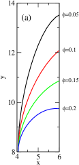
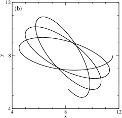
Figure 2: Weak field results. (a) The system was initialized as a Gaussian wavepacket of width $\sigma^{2}=5$, and kicked in the $+y$ direction at $t=0$ by applying a phase imprinting $\exp\left(iy\right)$. The center of mass of the wavepacket describes a circular orbit, the radius of which is inversely proportional to the effective flux, in analogy to the cyclotron orbit of a charged particle in a uniform magnetic field. (b) Here the system is initialized in the ground state of a parabolic trap potential $V=\kappa r^{2}/2$, with curvature $\kappa=0.1J$, which is then shifted 4 lattice spacings to the left. The center of mass traces out a rosette pattern, precisely analogous to the path of a Foucault pendulum subjected to the Coriolis force. Physical parameters: driving frequency $\omega=50J$, driving amplitude $K=0.05\omega$, and $n=1$.

For larger values of flux, when the magnetic length is comparable or less than the lattice spacing, the system’s behavior shows a complicated quantum interference pattern and it is no longer possible to use semiclassical intuition to understand it. As the Hamiltonian of the system is time-periodic, its dynamics is governed by its quasienergies $\epsilon_{j}$ hanggi . These are a generalization of the energy eigenvalues familiar from static systems, related to the eigenvalues of the time-evolution operator for one period $U(t+T,t)$ via $\lambda_{j}=\exp\left[-iT\epsilon_{j}\right]$. In Fig. 3a we show the quasienergy spectrum of the driven Hamiltonian for an $8\times 8$ lattice as $\Phi$ is varied from 0 to $2\pi$. In the upper figure the system is driven at a very high frequency $\omega=1000J$. The quasienergies clearly have the form of the Hofstadter butterfly, and indeed this spectrum is indistinguishable from the energy spectrum of the true (static) Harper-Hofstadter Hamiltonian hofstadter . We can distinguish two kinds of states. If more than $50\%$ of the wavefunction density is located on sites on the perimeter of the lattice we term the state an “edge state”, and otherwise it is termed a “bulk state”. The bulk states contain a self-similar series of gaps, which become fractal in the limit of large system size. The edge states, which would be absent in an infinite system or a system with periodic boundary conditions, lie within these gaps, and are chiral transporting states. It can be clearly seen that for a given value of flux the edge states occur in pairs with opposite slope, corresponding to propagation in either the clockwise or anti-clockwise sense around the boundary of the lattice.

In Fig. 3b we take the lower, and more experimentally realistic, value of $\omega=10J$ to demonstrate that our simulation procedure is robust. Reducing the value of $\omega$ affects the results in two ways; firstly the perturbation theory yielding Eq. (3) becomes increasingly less accurate, and secondly the error term arising from the Suzuki-Trotter decomposition (7) becomes more significant. These two sources of inaccuracy are responsible for the differences which Fig. 3b shows with respect to the ideal behavior of Fig. 3a. The butterfly structure is still clearly evident in the results, although some differences with the Harper-Hofstadter spectrum now appear. In particular we can observe that a subset of the edge states show an almost flat dependence on the flux, indicating that they have zero group velocity, and so are no longer transporting. Although these differences become more significant as $\omega$ is reduced further, we have checked that the broad structure of the Hofstadter butterfly is still reproduced even for driving frequencies as low as $\omega=2J$.

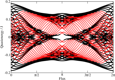
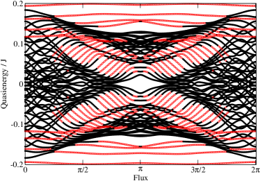
Figure 3: Quasienergy spectrum for high and low frequencies; black (solid) circles denote the bulk states, red (hollow) circles are states with more than 50% of their density localized on the edge. Driving parameters are $n=1$ and $K=0.1\omega$. (a) $\omega=1000J$, for this high frequency, the spectrum is indistinguishable from the “butterfly” spectrum of the true Hofstader-Harper Hamiltonian. (b) $\omega=10J$, some differences appear between the quasienergy spectrum and the Hofstadter butterfly; fewer edge states are visible, and a subset of edge states shows only a weak dependence on the magnetic flux.

Conclusions – In summary, we have described a method of using a periodic driving potential to produce a synthetic gauge field of arbitrary strength. To achieve this we have developed a split-driving approach, in which the desired time-evolution operator is constructed from a sequence of unitary operations that separate the $x$ and $y$ degrees of freedom. Our method is robust and simple, avoids the need for any additional fields and, unlike schemes based on hyperfine transitions, it does not require a specific internal structure for the atoms. It is also well within the reach of current techniques. For example, a typical optical lattice with $d_{L}\simeq 500$nm and bare tunneling $J/h\simeq 100$Hz can be driven at $\omega/2\pi\sim$1 kHz arimondo_Jn ; ketterle ; bloch , giving $\Delta t\sim$10 ms.

This method opens the prospect of using the single-site addressability and fine experimental control of cold atom systems to study the quantum Hall effect and topological insulator systems in a novel way. A particularly appealing application is to ladder systems belen , which provide a convenient bridge between one-dimensional topological insulators and the full two-dimensional case. Exciting future developments would be the generalization of these results to non-Abelian gauge theories, and to the rapidly developing field of Floquet topological insulators, in which the Floquet quasienergy spectrum itself has a non-trivial topology demler .

The authors thank Wolfgang Ketterle, Maciej Lewenstein, Juliette Simonet, and Monika Aidelsburger for stimulating discussions. This research was supported by the Spanish MINECO through Grant No. FIS-2010-21372.

References

- (1) I. Bloch, J. Dalibard, and S. Nascimbène, Nat. Phys. 8, 267 (2012).
- (2) B. Wunsch, F. Guinea, and F. Sols, New J. Phys 10, 103027 (2008).
- (3) L. Tarruell, D. Greif, T. Uehlinger, G. Jotzu, and T. Esslinger, Nature 483, 302 (2012).
- (4) L. Jiang, T. Kitagawa, J. Alicea, A.R. Akhmerov, D. Pekker, G. Refael, J.I Cirac, E. Demler, M.D. Lukin, and P. Zoller, Phys. Rev. Lett. 106, 220402 (2011).
- (5) D. Jaksch and P. Zoller, P. Ann. Phys. 315, 52 (2005).
- (6) D.R. Hofstadter, Phys. Rev. B 14, 2239 (1976).
- (7) Y. Lin, R.L. Compton, K. Jiménez-García, J.V. Porto, and I.B. Spielman, Nature (London) 462, 628 (2009); J. Dalibard, F. Gerbier, G. Juzeliūnas, and P. Öhberg, Rev. Mod. Phys. 83, 1523 (2011).
- (8) D. Jaksch and P. Zoller, New J. Phys. 5, 56 (2003); E.J. Mueller, Phys. Rev. A 70, 041603 (2004); F. Gerbier and J. Dalibard, New J. Phys. 12, 033007 (2010).
- (9) A. Celi, P. Massignan, J. Ruseckas, N. Goldman, I.B. Spielman, G. Juzeliūnas, and M. Lewenstein, Phys. Rev. Lett. 112, 043001 (2014).
- (10) K.W. Madison, F. Chevy, W. Wohlleben, and J. Dalibard, Phys. Rev. Lett. 84, 806 (2000); J. Abo-Shaeer, C. Raman, J. Vogels, and W. Ketterle, Science 292, 476 (2001).
- (11) F. Grossmann, T. Dittrich, P. Jung, and P. Hänggi, Phys. Rev. Lett. 67, 516 (1991).
- (12) H. Lignier, C. Sias, D. Ciampini, Y. Singh, A. Zenesini, O. Morsch, and E. Arimondo, Phys. Rev. Lett. 99, 220403 (2007).
- (13) C. Sias, H. Lignier, Y.P. Singh, A. Zenesini, D. Ciampini, O. Morsch, and E. Arimondo, Phys. Rev. Lett. 100, 040404 (2008).
- (14) C.E. Creffield, F. Sols, D. Ciampini, O. Morsch, and E. Arimondo. Phys. Rev. A 82, 035601 (2010).
- (15) C.E. Creffield and F. Sols, Phys. Rev. Lett. 100, 250402 (2008).
- (16) C.E. Creffield and F. Sols, Phys. Rev. A 84, 023630 (2011).
- (17) S. Longhi, Opt. Lett. 38, 3570 (2013).
- (18) J. Struck, C. Ölschläger, M. Weinberg, P. Hauke, J. Simonet, A. Eckardt, M. Lewenstein, K. Sengstock, and P. Windpassinger, Phys. Rev. Lett. 108, 225304 (2012).
- (19) P. Hauke, O. Tieleman, A. Celi, C. Ölschläger, J. Simonet, J. Struck, M. Weinberg, P. Windpassinger, K. Sengstock, M. Lewenstein, and A. Eckardt, Phys. Rev. Lett. 109, 145301 (2012).
- (20) A.R. Kolovsky, Europhys. Lett. 93, 20003 (2011).
- (21) C.E. Creffield and F. Sols, Europhys. Lett. 101, 40001 (2013).
- (22) H. Miyake, G.A. Siviloglou, C.J. Kennedy, W.C. Burton, and W. Ketterle, Phys. Rev. Lett. 111, 185302 (2013).
- (23) M. Aidelsburger, M. Atala, M. Lohse, J.T. Barreiro, B. Paredes, and I. Bloch, Phys. Rev. Lett. 111, 185301 (2013).
- (24) L. Wang and M. Troyer, Phys. Rev. A 89, 011603(R) (2014).
- (25) A. Eckardt, T. Jinasundera, C. Weiss, and M. Holthaus, Phys. Rev. Lett. 95, 200401 (2005).
- (26) E. Haller, R. Hart, M.J. Mark, J.G. Danzl, L. Reichsöllner, and H.-C. Nägerl, Phys. Rev. Lett. 104, 200403 (2010).
- (27) K. Kudo and T.S. Monteiro, Phys. Rev. A 83, 053627 (2011).
- (28) This cancellation of phases is a general feature of lattices with parallel-sided plaquettes, such as square and hexagonal lattices. It does not, however, apply to triangular lattices, which is why a non-zero (albeit staggered) flux could be observed in Ref. eckardt2, .
- (29) A.S. Sørensen, E. Demler, and M.D. Lukin, Phys. Rev. Lett. 94, 086803 (2005).
- (30) This form of flipping the sign of the acceleration was used in the resonant driving experiments of Ref. arimondo_Jn, .
- (31) M. Suzuki, Phys. Lett. A 146, 287 (1990).
- (32) A.R. Kolovsky, F. Grusdt, and M. Fleischhauer, Phys. Rev. A 89, 033607 (2014).
- (33) S. Burger, F.S. Cataliotti, C. Fort, F. Minardi, M. Inguscio, M.L. Chiofalo, and M.P. Tosi, Phys. Rev. Lett. 86, 4447 (2001).
- (34) M. Grifoni and P. Hänggi, Phys. Rep. 304, 229 (1998).
- (35) D. Hügel and B. Paredes, arXiv:1306.1190
- (36) T. Kitagawa, E. Berg, M. Rudner, and E. Demler, Phys. Rev. B 82, 235114 (2010).