The environments of Ly $\alpha$ blobs I: Wide-field Ly $\alpha$ imaging of TN J1338-1942, a powerful radio galaxy at $z\simeq 4.1$ associated with a giant Ly $\alpha$ nebula

Abstract

We exploit wide-field Ly $\alpha$ imaging with Subaru to probe the environment around TN J1338–1942, a powerful radio galaxy with a $>100\,\rm kpc$ Ly $\alpha$ halo at $z=4.11$. We used a sample of Ly $\alpha$ emitters (LAEs) down to $\log(L_{\rm Ly\alpha}[{\rm\,erg\,s^{-1}}])\sim 42.8$ to measure the galaxy density around TNJ1338, compared to a control sample from a blank field taken with the same instrument. We found that TNJ1338 resides in a region with a peak overdensity of $\delta_{\rm LAE}=2.8\pm 0.5$ on scales of $8\,h^{-1}\rm Mpc$ (on the sky) and $112\,h^{-1}\rm Mpc$ (line of sight) in comoving coordinates. Adjacent to this overdensity, we found a strong underdensity where virtually no LAEs are detected. We used a semi-analytical model of LAEs derived from the Millennium Simulation to compare our results with theoretical predictions. While the theoretical density distribution is consistent with the blank field, overdense regions such as that around TNJ1338 are very rare, with a number density of $6.4\times 10^{-8}\rm Mpc^{-3}$ (comoving), corresponding to the densest $<0.4$ percentile at $z\simeq 4.1$. We also found that the Ly $\alpha$ luminosity function in the TNJ1338 field differs from that in the blank field: the number of bright LAEs ($\log(L_{\rm Ly\alpha}[{\rm\,erg\,s^{-1}}])\ga 43.3$) is enhanced, while the number of fainter LAEs is relatively suppressed. These results suggest that some powerful radio galaxies associated with Ly $\alpha$ nebulae reside in extreme overdensities on $\sim 3$–$6\,\rm Mpc$ scales, where star-formation and AGN activity may be enhanced via frequent galaxy mergers or high rates of gas accretion from the surroundings.

1 Introduction

Galaxies are thought to form through accretion of baryonic material (Pre-Galactic Medium, PGM) from their surrounding environment, which provides the cold gas necessary for the star-formation process to proceed. The classical picture of this accretion is that the PGM is immediately heated to the virial temperature of the dark haloes (typically $\sim 10^{6}$ K) to form hot haloes (e.g. rees1977). Recent theoretical studies, in contrast, predict that cold gas accretes in the form of cold flows (with temperatures of $\la 10^{5}$ K) which penetrate the hot haloes surrounding the galaxies and which over cosmic time maintain the star-formation activity in galaxies (e.g. keres2005; dekel2009). At these low temperatures the gas in the PGM will predominantly cool via Ly $\alpha$ emission. The star-formation episodes powered by this accretion in turn provide a stellar feedback mechanisms which can then re-heat and eject material in the form of galactic-scale outflows (galactic winds: e.g. veilleux2005; steidel2010), which subsequently interact with the ambient material in the Circum-Galactic Medium (CGM). Hence both the accretion and outflows mean that galaxies interact with their surrounding environments, potentially resulting in extended Ly $\alpha$ emission either through cold accretion of the PGM (e.g. fardal2001; dijkstra2006; dijkstra2009; faucher-giguere2010; goerdt2010), or from galactic winds ejected into CGM (e.g. tenoriotagle1999; taniguchi2000; mori2006; dijkstra2012). Such Ly $\alpha$ nebulae may therefore reflect either the structure of the surrounding material, or gas circulation processes during the formation/evolution of these galaxies (furlanetto2005).

The precise mechanisms responsible for forming Ly $\alpha$ nebulae are still unclear. Some Ly $\alpha$ nebulae (e.g., those in the SA 22 protocluster at $z=3.1$) have been extensively observed, and are thought to be driven by starburst events in massive galaxies forming galactic winds (e.g. ohyama2003; wilman2005; matsuda2006; geach2005; geach2009; uchimoto2008; uchimoto2012). Moreover, recent surveys targeting Ly $\alpha$ “blobs” have also suggested a possible connection between their properties (specifically morphologies) and the environments they reside in (erb2011; matsuda2011; matsuda2012). Such an environmental dependence is also qualitatively consistent with the observations of relatively isolated Ly $\alpha$ nebulae, which may point to the possibility that these are accretion-driven (nilsson2006; smith2007; saito2008). However, to determine the true significance of environment in the formation of extended Ly $\alpha$ emission haloes, more detailed and systematic observations with sufficient depth and area are essential.

It has been long known that powerful radio galaxies at high redshifts are often associated with large, extended Ly $\alpha$ nebulae (e.g. chambers1990; rottgering1995; vanojik1996; vanojik1997; venemans2007; villar-martin2007). Although these Ly $\alpha$ nebulae appear linked to the radio emission, their properties are similar to the Ly $\alpha$ blobs described above. For example, the large velocity widths exceeding $\sim 1000\rm\,km\,s^{-1}$ (vanojik1997) or absorption across the full extent of the Ly $\alpha$ nebulae (rottgering1995; vanojik1996) are also seen in the Ly $\alpha$ nebulae in protoclusters (e.g. wilman2005; matsuda2006). Furthermore, observational studies suggest that large fraction of very luminous Ly $\alpha$ blobs ($\ga 10^{44}{\rm\,erg\,s^{-1}}$) are likely to be driven by obscured AGNs (e.g. colbert2011; overzier2013). There appears to be a size dependence of the Ly $\alpha$ nebulae on the size of radio sources (vanojik1997), as well as a hint of environmental dependence on the size of the Ly $\alpha$ nebulae (venemans2007). Even for those Ly $\alpha$ blobs not directly associated with radio sources, these are sometimes found to be harbouring AGNs (e.g. basu-zych2004; geach2009). These results suggest that Ly $\alpha$ nebulae are common phenomena reflecting the interaction between massive galaxies and their surrounding environments, regardless of the presence of AGNs. It is thus quite essential to probe the environments of Ly $\alpha$ nebulae with and without radio sources.

We have conducted a systematic, wide-field imaging observations of the environments around known giant Ly $\alpha$ nebulae, as traced by Ly $\alpha$ emitters (LAEs). Here we present the results from the imaging of the first target, the powerful radio galaxy TN J1338–1942 (hereafter TNJ1338) located at $z=4.11$ (debreuck1999). This radio galaxy is known to have a Ly $\alpha$ nebula extending up to $\sim 100\,\rm kpc$ with an asymmetric morphology (venemans2002). It has been suggested that this source is associated with a highly overdense region traced by LAEs and Lyman break galaxies, and thus represents an ancestor of present-day clusters, i.e., a protocluster (miley2004; venemans2002; venemans2007; intema2006; overzier2008). Theoretical simulations also suggests that the overdensity associated with TNJ1338 is likely to be an ancestor of a present-day cluster (chiang2013). Multiwavelength observations have shown that this source has radio lobes with an extent of $\sim 70\,\rm kpc$. (debreuck2004; venemans2007). The extended Ly $\alpha$ nebula around this source has signatures of star-formation induced by the radio jet, well outside the host galaxy at radii of $\sim 20$ kpc or more (zirm2005). Finally, Chandra X-ray observations indicate that there is weak extended emission ($\sim 30\,\rm kpc$) which may arise from inverse-compton scattering of cosmic microwave background or locally-produced far-infrared photons (smail2013).

Together these observations suggest a number of processes responsible for intense interaction between the central radio galaxy and the surrounding environment. However, due to the lack of the wide-field imaging data, the surrounding environment of this radio galaxy is still not well characterised. The existing LAE survey data cover a small field (two $7^{\prime}\times 7^{\prime}$) making it hard to map any overdensity, and there is no matched blank field observations which means that even the magnitude of the overdensity is uncertain. (venemans2007 used the Large-Area Lyman Alpha (LALA) survey results (rhoads2000; dawson2004) for the reference, which are taken with the different telescope and instrument, targeting a slightly different redshift). Accordingly the relationship between the structure hosting the radio galaxy (and the protocluster) and the wider surrounding environment cannot be probed with the existing data.

The goal of our study is to better quantify the environment of the powerful radio galaxy TNJ1338. To this end we have obtained wide-field intermediate-band images to identify the LAEs lying at the redshift of the radio galaxy, and so quantify the environment using the LAE number density. The magnitude of the overdensity was determined from comparison with a control sample taken from a blank field, SXDS (furusawa2008), at the same redshift and with the same instrumental setup (saito2006). This enables us to probe “on what scale does a significant overdensity exist?”, i.e., the amplitude of the overdensity and the spatial extent of the protocluster. We also compare our observations with predictions derived from combing the Millennium Simulation (springel2005) with a semi-analytical model for LAEs (orsi2008). This allows us to estimate how rare is the overdensity found around the radio galaxy, and more generally how well the simulation can reproduce such environments. This is the first truly panoramic ($\sim 30^{\prime}\times 30^{\prime}$) systematic and quantitative study of the environment of a radio galaxy field at $z\sim 4$.

The rest of this paper is organized as follows: We introduce the data and observational details in §2. The procedure to select LAEs from these data are presented in §3. In §4, we compare the observed density field and luminosity function of LAEs in the radio galaxy field and the blank field, and then compare the observations to the mock LAEs from the theoretical simulations. Throughout this paper, we use the standard $\Lambda$CDM cosmology with $\Omega_{M}=0.3,$$\Omega_{\Lambda}=0.7$, $H_{0}=100h=70\rm km\,s^{-1}Mpc^{-1}$, unless otherwise noted. All the magnitudes are in AB system (oke1974; fukugita1995).

2 The data

Table 1: Summary of Observations

Filter	$\lambda_{\rm cent}$/$\Delta\lambda$ ${}^{a}$	Exposure Time	$m_{5\sigma}$ ${}^{b}$	PSF ${}^{c}$
	[Å/Å]	[sec]	[AB mag]	[${}^{\prime\prime}$]
IA624	6226/302	28800 ($1800\times 16$)	26.94	0.74
$B$	4417/807	4800 ($1200\times 4$)	26.87	0.80
$R$	6533/1120	5940 ($540\times 11$)	26.92	0.55
$i^{\prime}$	7969/1335	2700 ($300\times 9$)	26.56	0.64
$BR^{d}$	6226/1927	–	26.90	0.74

${}^{a}$The central wavelength and FWHM of the filters.

${}^{b}$The $5\sigma$ limiting magnitudes within a $1.5^{\prime\prime}$ diameter aperture.

${}^{c}$The median PSF size (FWHM).

${}^{d}$The weighted mean of the $B$ and $R$-band images.

2.1 Subaru imaging data

We obtained 8.0 hours integration through the IA624 intermediate-band filter centred at $(\alpha,\delta)=(13^{h}38^{m}13.9^{s},-19^{\circ}42^{\prime}29^{\prime\prime})$ (J2000.0) on 2008 May 31 and June 01 (UT) with Suprime-Cam (miyazaki2002) on the 8.2-m Subaru Telescope (iye2004), under the proposal ID S08A-072 (PI: Y. Matsuda). For the continuum correction we obtained archival broad-band imaging in the $B$ and $R$-bands taken by intema2006 from the archive system SMOKA (baba2002). The archival $i^{\prime}$-band data by the same observers were also obtained to check the contamination using the continuum colour. Details of the observations are summarized in Table 1. Suprime-Cam has a pixel scale of $0^{\prime\prime}.202$ and a field of view of $34^{\prime}\times 27^{\prime}$. The intermediate-band filter, IA624, has a central wavelength of 6226Å and bandwidth of 302Å (FWHM), which corresponds to the redshift range for Ly $\alpha$ at $z=3.996$–$4.245$ (R23 IA filter system: hayashino2000; taniguchi2004). Fig. 1 shows the transmission curves of the IA624, $B$ and $R$-band filters, and the observed-frame wavelength of the Ly $\alpha$ line at the redshift of TNJ1338 ($z=4.11$).

The raw data were reduced with sdfred20080620 (yagi2002; ouchi2004) and iraf. We flat-fielded using the median sky image after masking sources. We then subtracted the sky background adopting a mesh size of 64 pixels ($13^{\prime\prime}$) before combining the images. Photometric calibration was obtained from the spectroscopic standard stars, PG1323$-$086, and PG1708+602 (massey1988; stone1996). The magnitudes were corrected for Galactic extinction of $E(B-V)=0.10$ mag (schlegel1998). The variation of the extinction in this field is sufficiently small ($\pm 0.01$ mag from peak to peak) that it does not affect our results.

The combined images were aligned and smoothed with Gaussian kernels to match their PSF to a FWHM of $0^{\prime\prime}.74$. The PSF sizes for some exposures in the $B$ band were not as good as the other bands (the median PSF size was $0.8^{\prime\prime}$), so that we removed these bad-seeing data, using only the four best frames for our analysis. The total size of the field analysed here is $32^{\prime}\times 24^{\prime}$ after the removal of low-S/N regions near the edges of the images. We also masked out the haloes of the bright stars within the field, resulting in the effective area of 689 arcmin${}^{2}$ in total. This corresponds to a comoving volume of $1.7\times 10^{5}h^{-3}\rm Mpc^{3}$ at $z=4.1$, covering a radial comoving distance of $112.4\,h^{-1}\rm Mpc$ for sources with Ly $\alpha$ emission lying within the wavelength coverage of the IA624 filter.

The blank-field data used for the control sample were taken as part of the Subaru/XMM-Newton Deep Survey (SXDS) project (furusawa2008) and a subsequent intermediate-band survey (saito2006). The SXDS field consists of five pointings, centred at $(\alpha,\delta)=(02^{h}18^{m}00.0^{s},-5^{\circ}00^{\prime}00.0^{\prime\prime})$ (J2000). The intermediate-band (including IA624) data were taken only in the south field (SXDS-S) centred at $(\alpha,\delta)=(02^{h}18^{m}00.0^{s},-5^{\circ}25^{\prime}00.0^{\prime\prime})$ (J2000). The data were taken with the same instrument on the same telescope, and reduced in the same manner with the same software as our TNJ1338 observations. The PSF was matched to $0^{\prime\prime}.78$ (FWHM), and the $5\sigma$ limiting magnitudes are 26.60, 27.42 and 27.91 for the IA624, $B$ and $R$, respectively. After masking out the regions near the edges and bright stars, the total area coverage was 691 arcmin${}^{2}$, which is almost the same as the TNJ1338 field.

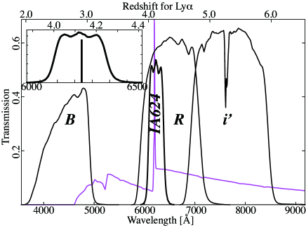
Figure 1: The response curves of our filters. The transmission of the filters are plotted against the wavelength. The lower axis shows the observed wavelength, and the upper axis gives the corresponding redshift for Ly $\alpha$ line. The thick black curve shows the intermediate-band filter (IA624) used to select sources with Ly $\alpha$ emission. The two broadband filters (B and R) are shown with thin lines. The thick magenta curve shows a model SED of a star-forming galaxy created with GALAXEV (bc03) with a Gaussian-profile Ly $\alpha$ emission line, redshifted to $z=4.1$. The box in the upper-left shows a close-up view of the IA624 filter transmission, together with the redshift of TNJ1338 indicated with a vertical thick bar.

2.2 Mock catalogue of Ly $\alpha$ emitters

In order to compare the observations with the predictions from a cosmological $N$-body simulation (Millennium Simulation: springel2005), we exploited a LAE catalogue generated with a semi-analytical model of galaxy formation (GALFORM cole2000; ledelliou2005; ledelliou2006). This catalogue contains $\sim 10^{6}$ LAEs with a wide range of luminosity and the Ly $\alpha$ equivalent widths (EWs). The details of this catalogue are described in orsi2008. The LAEs in this catalogue were generated by placing model galaxies into dark haloes of masses above the threshold value appropriate for the simulation’s mass resolution. The star-formation history for each halo was calculated by using a Monte-Carlo merger tree. The IMF was assumed to be top heavy for those stars formed during any starbursts, $dN/d\ln(m)\propto m^{-x}$ with $x=0$, with a standard solar neighbourhood IMF (kennicut1983) for those stars which quiescently form in discs, i.e. $x=0.4$ for $m<1M_{\odot}$ and $x=1.5$ for $m>1M_{\odot}$. Both IMFs covers the stellar-mass range $0.15\,M_{\odot}<m<125\,M_{\odot}$. The Ly $\alpha$ line luminosity is then calculated from the number of ionising photons emitted by the corresponding stellar population.

orsi2008 compared the properties of model LAEs from their simulation with existing LAE surveys and showed that both the luminosity function (LF) and the clustering properties are broadly consistent with the observations. The number density of model LAEs in the luminosity range of $\sim 10^{42.5}$–$10^{43}{\rm\,erg\,s^{-1}}$ are slightly higher than observed in the SXDS at $z=3.1$, but slightly below the SXDS at $z=5.7$. The difference is up to $\sim 0.5\,\mbox{dex}$, so that the accuracy of the model prediction for the LFs should be around $\sim\pm 0.5\,\mbox{dex}$. From this catalogue we selected LAEs using similar colour constraints to those applied to the observed data, see §3 for details of the selection procedure.

3 Sample selection

3.1 The TNJ1338 field sample

We used the IA624 image for detection, and the wavelength-weighted mean of $B$ and $R$ band images (hereafter BR) to determine the continuum level at a rest-frame wavelength of 1216Å. The BR image was generated by combining the two images with:

$$BR=\frac{(\lambda_{Ly\alpha,\rm obs}-\lambda_{B})R+(\lambda_{R}-\lambda_{Ly\alpha,\rm obs})B}{\lambda_{R}-\lambda_{B}}$$

where $\lambda_{B}$ and $\lambda_{R}$ are the central wavelengths of $B$ and $R$ bands, respectively, and the $\lambda_{Ly\alpha,\rm obs}$ is the observed-frame wavelength of the Ly $\alpha$ line at $z=4.11$. The source detection and photometry were made using the source- detection and classification tool, SExtractor (bertin1996). The sources detected here have at least five connected pixels above a threshold corresponding to $1.5\sigma$ of the sky noise. Using the position of these sources detected in the IA624 image, photometry was measured in the other bands with the same aperture, after matching the PSF size. We measured photometry for a total of 205,011 sources, after masking.

Based on the photometry catalogue from these three images ($B$, $R$, and IA624: $i^{\prime}$ was not used for the selection since the data is rather shallow), we selected the LAE candidates at $z\simeq 4.1$ by applying the following conditions.

$$20<{\it IA624}<26.6$$ (1)

$$BR-{\it IA624}>0.3$$ (2)

$$B>27.87,\mbox{ or, }B-R>2.17$$ (3)

$$BR-{\it IA624}>(BR-{\it IA624})_{4\sigma}$$ (4)

We first applied the magnitude cut (eq. 1) to remove bright foreground contaminants (${\it IA624}>20$) and a faint limit to remove false detections (${\it IA624}>5\sigma$). Note that the $5\sigma$ threshold here is set according to the SXDS data, not the TNJ1338 data, in order to make a fair comparison with the control sample obtained in the SXDS field. The bright threshold, 20 mag, was determined from visual inspection of the sources. This value roughly corresponds to Ly $\alpha$ luminosities corresponding to the brightest high-redshift radio galaxies (e.g., debreuck2001; reuland2003). Eq. 2 selects those sources with Ly $\alpha$ excess in the intermediate band filter, corresponding to an equivalent width of $\ga 200\rm\AA$ ($\ga 40\rm\AA$ in the rest frame). Then we applied a colour selection designed to detect the Lyman-break at $z\sim 4$ (eq. 3). Finally, eq. 4 requires that the IA624 excess has a significance level of at least $4\sigma$. Note that we used the $BR$ matched-continuum to estimate the IA624 excess, although the $B$ band should detect almost no flux from $z\sim 4$ sources because the wavelength coverage of the $B$ band is mostly below the Lyman limit. However, the distribution of the $R-{\it IA624}$ colour is not centred at zero, so that defining IA624-excess sources using just the $R$-band continuum level is somewhat unclear. We thus used the $BR$ to measure the continuum levels.

Fig. 2 shows the colour-magnitude diagram used for our LAE selection. We need to be aware of the possible contamination due to the noise in the IA624 excess measurements: the LAEs should lie well above the scatter around $BR-{\it IA614}=0$. For some cases, i.e., when the IA624 is relatively shallow, false detections may dominate sources selected at the $3\sigma$ level. We carefully visual inspected all the sources selected here, and we found two source that is obviously affected by bad regions of the CCD. These sources are in a region affected by a neighbouring bright source. Excluding this, we constructed a sample of 31 LAEs in the TNJ1338 field.

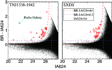
Figure 2: Colour-magnitude diagram. $BR-{\it IA624}$ colour as a function of IA624 magnitude for the TNJ1338 field. (Left) The black dots show all the sources, and the red triangles show $4\sigma$-excess LAE candidates. The vertical grey dashed line shows the magnitude cut (${\it IA624}>26.6$), the horizontal magenta dashed line indicates the $BR-{\it IA624}>0.3$ threshold. The red dashed curves show $4\sigma$ level of the IA624 excess. (Right) Same as the left panel, but for the SXDS blank field.

Fig. 3 shows the sky distribution of the LAEs selected above, overlaid on the IA624 image. The reader should note the apparent “void” around the north-western part of the field, where relatively few LAEs are detected, and does not seem to be an artifact of the bright stars.

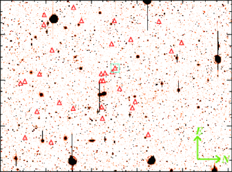
Figure 3: The sky distribution of our LAEs in the TNJ1338 field. The symbols for our photometrically-selected LAE sample are the same as Fig. 2, and the position of TNJ1338 is shown with the cyan box. The background is the IA624 image taken with Suprime-Cam. East is up, and north is to the right

The photometric properties of the sources selected here are summarised in Table 2. We here checked the overlap of our sample with previous studies. We cross-matched the coordinates of our sources with LAEs in the sample of venemans2007 and Lyman break galaxies (LBGs) in overzier2008, both observing the same field. We found three sources also included in the previous LAE sample, and four with the LBG sample. Furthermore, when we apply slightly looser colour constraint, $BR-{\it IA624}>3\sigma$ instead of the eq. 4, we have seven and eleven overlapped sources with the LAE- and LBG samples, respectively. This shows that our colour constraints (eq. 1-4) are working at least qualitatively well to select LAEs at $z\sim 4$. Since our redshift coverage is $\sim 5$ times wider than that of venemans2002; venemans2007, most of our sources are likely to be located outside the Venemans et al.’s coverage. Indeed, only three sources associated with the density peak around the radio galaxy (including the radio galaxy itself) are overlapped with the Venemans et al.’s sample. Our sample thus traces the overdense structure larger than $\sim 33(23\,h^{-1})$ comoving Mpc along the line of sight. Altough most of our sources do not overlap with the other samples of LAEs and LBGs, their UV ($R-i^{\prime}$) colours are fairly consistent with that expected for $z\sim 4$ galaxies. We computed the mean and the standard deviation of the $R-i^{\prime}$ colours of our and Venemans et al.’s samples of LAEs, and obtained the colour indices of $-0.14\pm 0.49$ and $0.19\pm 0.38$, respectively. Both of them agree with the $R-i^{\prime}$ colours of our SXDS control sample within the errors. We then extracted 11 sources with $i^{\prime}<26.0$ from our sample ($R-i^{\prime}$ colours of $0.08\pm 0.4$), and found that 10 of them satisfy the LBG selection criteria by ouchi2004. The remaining one source has slightly red $R-i^{\prime}$ colour, but fainter than $1\sigma$ level in $B$ band, which is consistent with the Lyman break feature. In any case, this source lies in relatively less-luminous range of the luminosity function of our sample, and is located in average-density region ($\sim 1.3\times$ the average). Even if this source is a foreground contaminant, our results thus does not significantly change. For the sources overlapped with the Overzier et al.’s LBG sample, all including the radio galaxy satisfy the colour constraints of LBG, showing that our colour selection is working quite well. We thus concluded that our sample does not contain significant contamination of the foreground sources.

Table 2: List of the photometrically-selected LAEs in the TNJ1338 field

ID	$\alpha$ (J2000)	$\delta$ (J2000)	IA624	$BR$	$B^{a}$	$R^{a}$	$i^{\prime a}$	$\log(L_{\rm Ly\alpha}[{\rm\,erg\,s^{-1}}])\,^{b}$	Notes
47564	$13:37:39.77$	$-19:51:57.4$	26.06	27.19	28.62	26.91	27.44	43.21
54822	$13:37:42.61$	$-19:55:48.4$	25.55	26.43	28.60	26.16	26.40	43.34
58749	$13:37:44.52$	$-19:37:37.8$	24.98	25.49	28.62	25.21	25.36	43.41
83374	$13:37:54.64$	$-19:44:22.8$	25.50	26.21	28.62	25.92	25.98	43.31
93306	$13:37:58.96$	$-19:54:02.5$	25.33	25.77	28.62	25.49	24.23	43.21
97780	$13:38:00.88$	$-19:48:41.8$	26.08	27.19	28.62	26.90	28.31	43.19
98384	$13:38:01.22$	$-19:39:58.1$	25.50	26.07	28.62	25.78	25.75	43.23
99860	$13:38:01.71$	$-19:44:29.6$	25.37	26.03	28.44	25.75	25.87	43.33
106649	$13:38:04.53$	$-19:50:44.9$	25.29	26.02	28.62	25.74	26.10	43.39
107660	$13:38:05.17$	$-19:39:32.6$	24.06	24.58	27.91	24.30	24.37	43.78
127592	$13:38:13.16$	$-19:41:50.0$	26.19	28.49	28.62	28.23	26.92	43.29
135689	$13:38:16.58$	$-19:56:29.3$	25.72	26.38	28.62	26.09	26.11	43.19
138350	$13:38:17.81$	$-19:55:49.6$	25.04	25.60	28.62	25.32	25.38	43.41
139312	$13:38:18.10$	$-19:44:37.0$	26.09	27.27	28.62	26.95	27.15	43.21
139843	$13:38:18.23$	$-19:44:14.1$	25.69	26.30	28.15	26.06	26.59	43.18
149890	$13:38:22.31$	$-19:53:40.2$	25.50	26.49	28.62	26.23	26.68	43.40
150274	$13:38:22.48$	$-19:44:33.7$	25.51	26.28	28.62	26.02	25.89	43.33	d,e
151277	$13:38:22.92$	$-19:43:59.3$	25.56	26.46	28.62	26.19	26.63	43.35	e
153858	$13:38:23.78$	$-19:42:56.8$	26.10	27.23	28.62	26.91	26.98	43.19	e
184585	$13:38:36.63$	$-19:34:11.3$	25.62	26.43	28.13	26.17	26.64	43.29
186397	$13:38:37.39$	$-19:51:48.8$	25.91	27.08	28.62	26.77	26.20	43.28
194782	$13:38:41.12$	$-19:43:01.9$	23.73	24.06	27.31	23.78	23.65	43.75	d
197870	$13:38:41.91$	$-19:32:41.1$	25.38	26.44	28.62	26.16	26.61	43.47
202840	$13:38:43.90$	$-19:40:11.5$	26.03	27.11	28.62	26.85	27.00	43.21
225768	$13:38:53.34$	$-19:53:01.1$	23.65	24.53	27.23	24.26	24.27	44.11
229080	$13:38:55.18$	$-19:36:02.4$	24.58	25.39	28.62	25.12	25.33	43.71
232509	$13:38:55.67$	$-19:42:36.9$	25.89	26.74	28.62	26.45	26.25	43.20
232582	$13:38:55.67$	$-19:47:27.7$	25.85	26.62	28.62	26.35	26.64	43.19
242571	$13:38:59.45$	$-19:52:57.5$	26.03	27.21	28.62	26.98	27.05	43.23
257624	$13:39:04.04$	$-19:48:38.6$	25.64	26.52	28.62	26.26	26.83	43.31
155683	$13:38:26.07$	$-19:42:30.5$	21.81	23.33	28.62	23.04	24.05	44.97	c,d,e

Notes: (a) Broadband magnitudes are replaced with the $1\sigma$ values when the photometry results are below the $1\sigma$ level; (b) Ly $\alpha$ line luminosities are estimated from the photometry by assuming that they are located at $z=4.1$; (c) Radio galaxy; (d) also included in the LAE sample of venemans2007; (e) also included in the LBG sample of overzier2008.

The expected contaminants are [O II]$\lambda 3727$ emitters at $z\sim 0.7$, and [O III]$\lambda\lambda$4959, 5007 emitters at $z\sim 0.25$. Although our selection corresponds to very large EWs, these contaminants cannot be ruled out simply by their EWs, as there are certain amount of such strong emitters (e.g. vanderwel2011; atek2011). The LFs of such strong emitters are still not studied well, but narrowband surveys can give a rough estimate of the number density of such populations. kakazu2007 pointed out that strong [O III] emitters are the most common among such strong smission line galaxies, and their [O III] LF gives the number density of the sources with EWs of $\log(\rm EW[\AA])\ga 2$ to be $\sim 1\times 10^{-3}\,\rm Mpc^{-3}$ at $z\sim 0.6$. If we assume that this density is valid for $z\sim 0.25$, the expected number of [O III]$\lambda$5007 within our survey volume is around unity, when integrating over the whole luminosity range of our sample. Even if other emitters ([O III]$\lambda$4959 and [O II]$\lambda$3727) have similar number density, only a few sources would be contained in our sample, which is quite unlikely. To test how the contamination affect our results, we reduced the number of sources by using $BR-{\it IA624}>5\sigma$ instead of eq. 4. This selection excludes one source lying within the high-density region around the radio galaxy, giving the peak overdensity well within the error. This does not make any significant changes in our results, i.e., the density field and the shape of the Ly $\alpha$ luminosity function.

3.2 The control sample in SXDS field

We constructed a control sample of LAEs, using similar imaging data in a blank field (the SXDS-S field, hereafter SXDS). These data were taken with the same instrument and filters as used in the TNJ1338 observations as noted above, and the field is not biased to any known overdense regions at $z\sim 4$. In order to make a fair comparison between the two fields, we defined the colour constraints based on the shallower data of the two, i.e., $5\sigma$ limiting magnitudes are assumed to be ${\it IA624}=26.60\,\rm mag$, $R=26.94\,\rm mag$, and $B=26.87\,\rm mag$. We also corrected for the offset of $BR-{\it IA624}$ colour distribution for the SXDS field, presumably due to an error in the magnitude zero point. We then applied a colour term $\Delta(BR-{\it IA624})=0.15$. This colour term was estimated by fitting a Gaussian function to the colour distribution. We derived the colour offset necessary to force the centre of the colour distribution to zero within the magnitude range $20<{\it IA624}<26.60$. Except for applying this colour term, we employed exactly the same colour constraints to select the LAEs in this field. The total number of sources identified is 34. The colour-magnitude diagram for this sample is shown in Fig.  2 together with the TNJ1338 sample.

3.3 The mock LAE sample

In order to make a meaningful comparison between the observations and the simulation, we selected LAEs from the mock LAE catalogue at $z=4.17$ described in §2, which is the output redshift closest to that of TNJ1338. We used the predicted Ly $\alpha$ fluxes and EWs contained in the catalogue, to calculate the colours and magnitudes of the LAEs. Note that the catalogue contains $z=4.17$ LAEs, while we are going to constrain the observed (apparent) colours of $z\approx 4.11\pm 0.12$. However, the difference between these two epochs is very small, $\sim 55\,\rm Myr$, and $z=4.17$ is well within the coverage of the IA624 filter. We thus calculated the apparent (observed) colours at $z=4.11$. This should be a reasonable assumption to compare the simulated LAEs with the observations, since the timescale of galaxy evolution (e.g., star formation) is much longer than this difference.

We first calculated the absorption of the UV continuum by the intervening IGM, following the formalism of madau1995. Here the UV continuum was assumed to be flat in terms of flux density per unit frequency bin, $f_{\nu}=\mbox{\rm Const}$. The flux density was obtained by dividing the Ly $\alpha$ flux by EW (observed), $f_{\lambda}=F({\rm Ly\alpha})/W_{obs}$. Then the IGM absorption was calculated by assuming the redshift of $z=4.11$ to obtain the continuum component of the spectrum expected at the redshift of the radio galaxy. The UV continuum contribution to the photometry was calculated by convolving the flat-continuum spectrum with the filter response curves. The IGM absorption on the Ly $\alpha$ line is included in the escape fraction, $f_{esc}$ used in generating the mock catalogue of LAEs (see orsi2008). Then sufficiently narrow line profiles (i.e., narrower than the IA624 passband) was convolved with the filter response curves, and the line contribution to the photometry was obtained.

Adding the contributions from both the Ly $\alpha$ line and the UV continuum, we calculated the $R$- and IA624 band magnitudes to apply the colour constraints. Since our calculation gives exactly the same continuum colour for all sources, we did not apply the constraints on the $B-R$ colour. This does not affect our results because the mock LAE catalogue does not contain any foreground contamination. Furthermore, the $B$-band magnitude cannot be predicted from our calculation with sufficient reliability, because we are assuming a very simple IGM absorption model. Due to the Lyman-break feature and the Gunn-Peterson trough, the high-$z$ sources are expected to be fainter in $B$ than in the $R$ band. We indeed required in eq. 3 that $B-R>2.17$, which leads to be $\ga 0.15$ fainter $BR$ magnitudes than the $R$. In order to put the same colour- and magnitude constraints as for the observed samples, we then put the offset of $+0.15$ mag on the $R$-band magnitudes when computing the IA624 excess, instead of using $BR$ magnitudes. This gives the following criteria for selecting the LAEs:

$$20<{\it IA624}<26.6$$ (5)

$$R-{\it IA624}>0.15$$ (6)

$$R-{\it IA624}>(BR-{\it IA624})_{4\sigma}.$$ (7)

For the significance level of the IA624 excess, $(BR-{\it IA624})_{4\sigma}$, the same value as in eq. 4 was used to match the observed sample. For the comparison with the observed samples, we applied the magnitude cut of ${\it IA624}<26.6$ for eq. 5, and the observed IA624-excess threshold of $(BR-{\it IA624})_{4\sigma}$. In total we select 59,639 model LAE sources in a comoving volume corresponding to $(500\,h^{-1}\rm Mpc)^{3}$.

4 Results and discussion

4.1 Density field

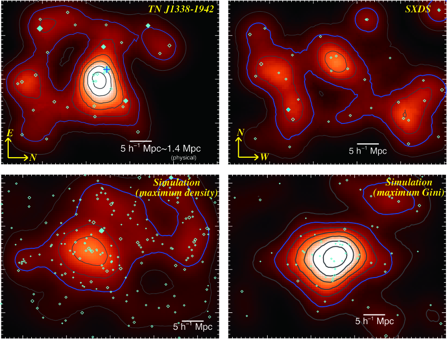
Figure 4: A comparison of the density field of LAEs. The top panels are the observed density map of the TNJ1338 field (left), and the SXDS field (right). The position of the radio galaxy TNJ1338 is shown with the blue cross mark near the density peak. The bottom panels are simulated density maps generated from the mock LAE catalogue using the same selection as those applied to the observed data, showing the same FoV centred on density peaks which are higher than that measured at the position of the radio galaxy: the field around the maximum density peak (left) and the field with the highest Gini coefficient (right). Each panel shows the $50\times 38\,h^{-2}\rm Mpc^{2}$ (comoving) field. The contour interval is $0.5\times$ the average density over the same FoV, with a lowest contour of 0.5 ($\delta_{\rm LAE}=-0.5,0.0,0.5,1.0,\dots$). The thick blue contour traces the average density over the field ($\delta_{\rm LAE}=0.0$). The cyan diamonds mark the positions of LAEs, and the sizes of these symbols represent the Ly $\alpha$ luminosities. The sources with $\log(L_{\rm Ly\alpha}[{\rm\,erg\,s^{-1}}])\ga 43.6$ are marked with filled symbols.

4.1.1 The high density region around the radio galaxy

We quantified the difference between the TNJ1338 and SXDS fields by constructing their LAE surface density maps. We smoothed the spatial distribution of the LAEs with a Gaussian kernel with a radius (half width at half maximum, HWHM) of $4\,h^{-1}\rm Mpc$ (projected comoving distance at $z=4.1$, corresponding to the physical distance of 1.1 Mpc), and counted the number of LAEs within the same radius at each grid point, with a grid spacing of $0.5\,h^{-1}\rm Mpc$. Then the surface density was obtained by dividing the number by the area of the Gaussian aperture with the HWHM of $4\,h^{-1}\rm Mpc$. In deriving the average surface density, the areas within $5\,h^{-1}\rm Mpc$ of the edge of the FoV were flagged to avoid underestimating the surface density near the field edges. The kernel size was chosen based on the typical separation between the sources. We measured the distance to the nearest source for each LAE in our sample, and chose the smoothing kernel size to include $\sim 68$ percent of the whole sample. We confirmed that different sizes of the smoothing kernel also give a similar density distribution. Note that the radio galaxy itself was excluded in creating the density map, since we are aiming to investigate the surroundings of the radio galaxy.

The density maps we obtained are shown in the Fig. 4. We can clearly see that the region around the radio galaxy is strongly overdense, and equivalently strong density peaks are not seen in the SXDS field. The density peak in the TNJ1338 field is $\approx 4$ times the density averaged over the field, while the maximum peak in the SXDS field is only $1+\delta_{\rm LAE}=2.36$. We then estimated the uncertainty of the density with this smoothing scale by computing the standard deviation of the density map of the SXDS field, determining the $1\sigma$ dispersion in $\delta_{\rm LAE}$ as 0.47. The radio galaxy TNJ1338 is located in the densest region in the field, with $1+\delta_{\rm LAE}=2.91$ at its position. The peak density is $1+\delta_{\rm LAE}=3.80$, located $2.8\,h^{-1}\rm Mpc$ offset from the position of the radio galaxy. This overdensity can be traced on $\sim 10$–$20\,h^{-1}\rm Mpc$ scales around the radio galaxy ($\sim 3$–$6\,\rm Mpc$ in physical). Outside this region, in contrast, the density appears to drop quite rapidly: on the northwestern side of the field there is a strongly underdense region just $\sim 20\,h^{-1}$ Mpc from the density peak. Such a strong variation in the density of LAEs is not seen in the SXDS field. Although the overdensity of the TNJ1338 field had previously been suggested by venemans2002, their FoV was much smaller than ours, and they were forced to estimate the overdensity (a factor of $\sim 3$–5) through comparison to a separate field survey at a similar redshift (rhoads2000). With our wide-field imaging of this field, we have not only confirmed the overdensity by comparing with an identically-observed control field, but have also determined the spatial scale and structure of the overdense region.

The difference between the TNJ1338 field and SXDS control field becomes clearer when comparing their density histograms, as shown in Fig. 5. In the SXDS field the distribution is concentrated near the average value, while the TNJ1338 field shows a much broader distribution extending toward both high- and low densities. In order to quantify the difference between the distributions in these two fields, we first compared the 10- and 90 percentiles for the density maps of the two fields. The upper panel of Fig. 5 shows the cumulative density distributions for the two fields, together with the percentiles. The statistics of the two fields are also summarised in Table 3. The TNJ1338 field has a wider density distribution compared with the SXDS field, especially at the lower-density end. The 10 percentile for the TNJ1338 field is $1+\delta_{\rm LAE}=0.05$, which is eight times lower than that of the SXDS field. The ratios of the two (10 and 90) percentiles, i.e., the dynamic range of the density, for the TNJ1338 and the SXDS fields are 37 and 4.2, respectively. The TNJ1338 field has thus nearly an order of magnitude higher range in galaxy density than that seen in the SXDS field. The difference becomes even more obvious when we look into the highest- and the lowest-density bins: e.g., $1+\delta_{\rm LAE}<0.01$ corresponds to the lowest 9.5 percent of density cells in the TNJ1338 field, while in the SXDS field only $\sim 0.2$ percent of the total grid points have such a low density.

A useful statistic to quantify the range of the density distribution is the Gini coefficient of the density field. The Gini coefficient, $G$, measures how uniformly LAEs are distributed within the field, and takes a value of $0<G<1$. The $G$ value corresponds to the area surrounded by the two Lorentz curves corresponds to the given distribution and $G=0$ (shown in Fig. 5). If all the LAEs are concentrated within one grid point, then $G$ is unity. If the LAEs are distributed uniformly over the field, then $G$ is zero. The Lorentz plot shown in Fig. 5 clearly shows that the TNJ1338 field has much higher $G$ than the SXDS blank field, and the blank field agrees well with the simulation. The Gini coefficients of the density maps were calculated to be 0.402 (0.268) for the TNJ1338 (SXDS) field. This difference shows that the LAEs are more concentrated into high-density regions (especially into the high-density peak around the radio galaxy) in the TNJ1338 field, compared with the SXDS field. Together these statistics suggest that the galaxy density in the TNJ1338 field traced with LAEs is highly concentrated within the high-density region near the radio galaxy, but that there are also unusually low-density regions in the field where the number of LAEs is highly suppressed. This is quite different from the density field in the SXDS field.

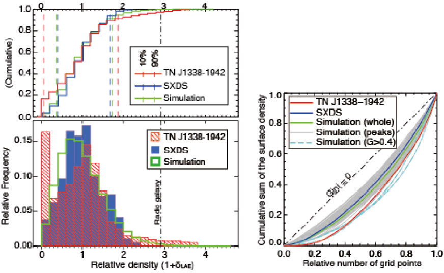
Figure 5: The statistics for the LAE surface density distribution. (Left) A comparison of the LAE surface density distributions for the two fields. The red hatched and the blue filled histograms show the density distribution for the TNJ1338 field and the SXDS control field, respectively. Overplotted with the thick green line is the histogram for the simulated density map obtained from the mock LAE sample. The vertical black dot-dashed line shows the density calculated at the position of the radio galaxy. The cumulative distributions are shown on the top panel. The red, blue and green lines denote the TNJ1338 , the SXDS and the simulated map, respectively. The 10-th and 90-th percentiles are shown with the vertical dashed lines with the corresponding colours. We can see that the density distribution in the TNJ1338 field is much wider than that in the SXDS. The simulated density distribution is closer to the SXDS than to the TNJ1338 field. (Right) Lorentz curves for the density distribution. The normalised cumulative distribution is plotted against the normalised number of the grid points. The red, blue and green curves show the TNJ1338, the SXDS and the simulated map, respectively. Again the simulated distribution is closer to that of the SXDS field rather than the TNJ1338 field. The grey curves denote the 94 fields centred at the high-density peaks found in §4.3.1, of which 21 have $G$’s higher than that of the whole simulated map. The three fields with the largest $G$’s among the 94 ($G\geq 0.4$) are shown with the cyan dashed curves. The TNJ1338 field has much higher $G$ than most of the high-density fields found in the simulation: only two out of 94 has higher $G$’s compared with the TNJ1338 field.

Table 3: Statistics of the observed density field

Field	Mean ${}^{a}$	Peak ${}^{b}$	Percentiles ${}^{c}$			$G$ ${}^{d}$
	$[h^{2}\rm Mpc^{-2}]$		10	50	90
TNJ1338	0.0201	3.80 (3.73)	0.05	0.98	1.86	0.402
SXDS	0.0204	2.36	0.40	0.97	1.68	0.268

${}^{a}$Mean surface density over the field in comoving scale.

${}^{b}$Peak normalised surface density ($1+\delta_{\rm LAE}$). The value normalised with the average of SXDS field is shown in the parenthesis.

${}^{c}$In units of the normalised density $(1+\delta_{\rm LAE})$.

${}^{d}$Gini coefficient of the density distribution.

4.1.2 Density contrast within the TNJ1338 field

Although the TNJ1338 field has a very large dynamic range in LAE density, the average density of this field over the FoV of Suprime-Cam is still almost the same as that of the SXDS field. The average surface density of LAEs for these two fields are $0.0201\,h^{2}\rm Mpc^{-2}$ and $0.0204\,h^{2}\rm Mpc^{-2}$ for the TNJ1338 and the SXDS field, respectively. This suggests that the density traced by LAEs is almost uniform (within $\sim 2$ percent) at $\sim 50\,h^{-1}\rm Mpc$ scales, when the density field is averaged over $\sim 112\,h^{-1}\rm\,Mpc$ along the line of sight (both in comoving scale). Even with this smoothing, there is a significant overdensity around the radio galaxy, and a similarly significant underdense region just adjacent to it. This “void” region next to the high-density region corresponds to the peak of the density distribution near zero in the histogram (Fig. 5). The shape of this distribution is quite different from that for the SXDS field.

Due to the limited number of sources, $\sim 30$ in each field, it is not clear whether the underdense region is truly a void. However, the detectable (i.e., bright and large-EW) LAEs were not found in this region, especially in the north-western quarter of the field. This appears to be a real effect since there are no bright stars in this region that would significantly affect the detection and photometry, as seen in the Fig. 3. Such a large underdense region is not seen in the SXDS field, again showing that this radio galaxy field has an unusually high density contrast. The real density contrast in this radio galaxy field is possibly higher than estimated, since we are smoothing the spatial distribution along the line of sight as a result of the relatively wide redshift coverage of the IA624 filter. Although the apparent contrast would be enhanced due to the redshift-space distortion if the high-density region is actively accreting the material, such an effect is thought to be small because of the wide redshift coverage.

Such a large density contrast within a single field suggests that the high-density region around the radio galaxy is attracting material from well within the scale of the Suprime-Cam FoV ($38\times 50\,h^{-2}$ comoving Mpc${}^{2}$ on the sky, when the edges are flagged out), because the average density is almost the same as the blank field. If LAEs are tracing the matter distribution, then the surrounding dark haloes within this scale should have been merging into this overdensity. Since we do not have spectroscopic data for all the sources, we cannot draw any clear conclusions on the true spatial structure of the overdensity based solely on our current observations: it is not clear whether the density peak represents a single extremely overdense halo, or a less overdense filamentary structure elongated toward the line of sight (the latter case includes the case that two or more clumps are aligned along the line of sight). Nevertheless, the density contrast must have grown to a level high enough to form such a high density peak and a large void region. Even for the latter case, the high-density filament must have accreted material from its surroundings and grown to a sufficient length to evacuate the void region. Hence in both cases, the spatial extent of the high-density region should be fairly compact (or the filament should be narrow), as the TNJ1338 field shows a large void fraction and the high-density region extends only up to $\sim 20\,h^{-1}$ comoving Mpc ($\sim 6$ Mpc in physical units) scales.

This requires that matter is concentrated into a high-density region of $\sim 10$–$20\,h^{-1}$ comoving Mpc size ($\sim 3$–6 physical Mpc), well before the observed epoch of $z\sim 4.1$. Such a concentration should affect the star-formation and AGN activity of galaxies within the overdensity, in the form of, e.g., frequent galaxy mergers. This may therefore lead to an excess of massive galaxies harbouring active star-formation and/or AGN activity. The corresponding high matter concentration will also lead to a higher rate of gas accretion from the surrounding environment, again resulting in the enhancement of star-formation and AGN activity.

4.2 Luminosity function

4.2.1 Comparison with the blank field

As described above, we have found that the TNJ1338 field has a high density region around the radio galaxy, and a strong density contrast between this and the large void region just adjacent to the peak. To investigate the variation in the LAE LF Fig. 6 compares the Ly $\alpha$ LFs of the LAEs in the TNJ1338 and the SXDS fields. We can see that the faint-end slope of the LF in the TNJ1338 field is significantly shallower than the SXDS, below a Ly $\alpha$ luminosity of $\log(L_{\rm Ly\alpha}[{\rm\,erg\,s^{-1}}])\sim 43.3$. On the other hand, the LF in the SXDS field increases nearly monotonically down to our completeness limit, $\log L_{\rm Ly\alpha}\sim 42.8$, as the $L^{*}$ is still slightly below the faintest data point (ouchi2008, hereafter O08). In the TNJ1338 field, a similar trend can be seen in the LF for LAEs within the overdense region. We plotted the LF of the subsample of LAEs lying within regions with densities higher than the average of the whole Suprime-Cam field ($\delta_{\rm LAE}\geq 0$). The faint end of this LF agrees with that of the SXDS field, but has higher values than in the SXDS by up to an order of magnitude. Note that the radio galaxy itself ($\log L_{\rm Ly\alpha}\approx 45.0$) is excluded in the LFs plotted here. The LAE population in the TNJ1338 field is thus thought to be highly biased to bright sources, and the fraction of faint LAEs is reduced in this field. The shape of the bright end may suggest that our LAE sample consists of two different components, e.g., star-forming galaxies dominating the faint end, and AGN hosts dominating the bright end. This should be real even if the bright end contains foreground contamination. As mentioned in §3, the luminosity function of foreground sources suggests that the expected number of [O II] emitter is around unity, even when integrated down to our completeness limit. The number of LAEs with $\log(L_{\rm Ly\alpha})\ga 43.6$ is four in the TNJ1338 field (excluding the radio galaxy), while that in the SXDS field is only one. It is unlikely that more than one such bright foreground sources are included in our sample, and thus the enhancement of the bright LAEs is thought to be real.

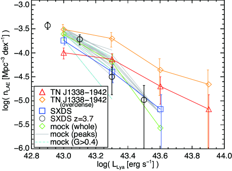
Figure 6: The Ly $\alpha$ luminosity function (LF) of the observed samples of LAEs. The red triangles show the LF of the total LAE sample in the TNJ1338 field. The subsample lying within the overdense regions (higher than the average of the field) is shown with the orange diamonds. The blue squares denotes the SXDS control sample. The black circles shows the LF of $z\simeq 3.7$ LAEs in the SXDS field, taken with a narrowband filter (ouchi2008). The green diamonds show the LF of the mock LAE catalogue by orsi2008, and the grey lines show the LF derived from the subsample of the mock LAEs residing within the Suprime-Cam-sized fields centred at the positions of 21 high-density peaks with high $G$’s. The LFs of the three highest-$G$ peaks among these 21 are marked with the cyan dashed lines. The radio galaxy TNJ1338 is omitted to show the luminosity range of the normal LAEs. Note that the data points are slightly shifted to improve the visibility. We can see that the number of bright LAEs is enhanced in the radio-galaxy field, and the fraction of the faint LAEs is reduced. The LF within the overdense regions has almost the same shape as that within the whole field, but the absolute number density agrees with that in the SXDS at a luminosity of $\log(L_{\rm Ly\alpha}[{\rm\,erg\,s^{-1}}])\sim 43.0$.

We have also compared the SXDS control sample with a narrowband-selected LAE sample at a similar redshift in the same field, to check the reliability of our control sample. The LF of the SXDS control sample agrees quite well with the LF of the narrowband-selected LAE sample at $z\simeq 3.7$ (O08), down to the completeness limit ($\log(L_{\rm Ly\alpha})\sim 42.8$). Since the bandpass of the IA624 filter is several times larger than the NB570 narrowband filter, the survey volume is comparable to that of O08, even with only one FoV of Suprime-Cam. This reduces the field-to-field variance, as the density fluctuations are smoothed out along the line of sight. Thus we confirmed that our SXDS sample is a valid control sample in terms of Ly $\alpha$ LF, representing the typical number density of LAEs at $z\sim 4$. The LF in the TNJ1338 field, on the other hand, lies beyond the variance expected from the results of O08. At the brightest end of the LF, $\log L_{\rm Ly\alpha}\ga 43.9$, we did not find any sources in the SXDS field, while we still found sources in the TNJ1338 field even when we exclude the radio galaxy itself. Such bright sources are almost never seen in blank-field surveys for LAEs at similar redshifts (dawson2007; ouchi2008).

These results reinforce the idea that the TNJ1338 field is unusual, not only in terms of the overdensity of LAEs, but also the Ly $\alpha$ LF. Since our IA624 data is deeper in the TNJ1338 field than in the SXDS field, this should not be due to the difference in the completeness. We mentioned in §4.1.2 that the density contrast in this field implies that the high-density region is accreting material from well within $\sim 50\,h^{-1}\rm Mpc$ scale. At this scale, such accumulation of the material is likely to be affecting the star-formation and/or AGN activity in galaxies and hence galaxy formation and evolution, leading to the enhancement of the bright end of the Ly $\alpha$ LF. The bright end of the Ly $\alpha$ LF is thought to be dominated by AGN hosts and/or actively star-forming galaxies, so that the formation of such “active” galaxies is likely to be enhanced in the TNJ1338 field.

4.2.2 Implications for galaxy formation

The high-density region around the radio galaxy is so unusual that it faces the large void region. The material originally in the void region must have moved into the surroundings by the epoch of $z\simeq 4.1$, and among the “surroundings”, the high-density region around the radio galaxy is the most prominent peak. This suggests that some large fraction of the material originally in the void region may have travelled to the vicinity of the radio galaxy. Then, how well can this scenario account for such a high density contrast as we found? We made a rough estimate to test this scenario. The separation between the density peak and the void region is $15-20\,h^{-1}\rm Mpc$ in comoving scale, which corresponds to $\sim 4-6\,\rm Mpc$ in physical scale at $z=4.1$. If the material travelled this distance within a Hubble time at this redshift, the velocity is required to be $\sim 4-6\times 10^{2}\rm km\,s^{-1}$. This is altough a very naive estimate, as is just the velocity required to travel linearly from the centre of the void to the density peak. In terms of the void evolution, the required velocity is slightly smaller: the apparent radius of the completely empty void is $r\sim 2-3\,\rm Mpc$, leading to the peculiar velocity at the edge of the void is around $\frac{1}{3}H(t)r\sim 2-3\times 10^{2}\rm km\,s^{-1}$. These values are well below the typical velocity dispersion of the present-day (virialised) galaxy clusters. Although the required peculiar velocity may be larger than this because the distance assumed here is just the projected distance, the high-density region can be to some extent responsible for accreting the material initially in the void region.

It is however quite unlikely that all of the material initially in the large void had been simply accreted onto the high-density region by the epoch of $z\simeq 4.1$. The material should in principle flow out in all directions from the centre, so that the single overdense region cannot be fully responsible for the formation of the void. The simplest interpretation for the observed (apparent) density contrast is that the initial density fluctuation is quite large, and the contrast had existed since an epoch well before $z\simeq 4.1$. Another interpretation is the enhancement of star-formation activity within overdense regions (e.g. steidel2005; koyama2013), leading to the enhancement of actively star-forming galaxies possibly dominating the bright end of the LF. This may result in a drastic enhancement of the galaxy bias for bright sources. The excess of extreme starbursts within protoclusters found in some observational studies (e.g. blain2004; capak2011; ivison2013) is consistent with this idea. Because of the lack of spectroscopic data, we cannot discriminate between star-formation and AGN activities. It is thus also possible that AGNs are dominating the bright end of the LF, which is highly enhanced in the radio galaxy field. Such an enhancement of AGN activity in overdense environments has been found observationally in some cases (e.g. pentericci2002; croft2005; lehmer2009; digby-north2010). Since our samples are relatively biased to bright LAEs, such effects will enhance the apparent density contrast.

The difference between the LFs in the two fields depends strongly on the luminosity. When we examine the LF for the overdense regions in the TNJ1338 field, the difference for the luminosity range $\log L_{\rm Ly\alpha}\ga 43.3$ (corresponding to the brightest two data points for the SXDS field) is about an order of magnitude. This luminosity range contains 15 sources for the TNJ1338 field (all in the overdense regions), while only 7 lie within this range in the SXDS field. On the other hand, both LFs agree with each other within their error bars (factor of $\sim 1.6$) at $\log L_{\rm Ly\alpha}\sim 43.0$. The difference in the faintest data point roughly corresponds to the difference in the total number density for the two fields (the whole SXDS field and the overdense region of the TNJ1338 field). We estimated that the mean density within the overdense regions shown here is $\sim 1.6$ times the average of the SXDS, corresponding to $\delta_{\rm LAE}\sim 0.6$. Since the LF for the overdense regions in TNJ1338 exceeds the LF in the SXDS field by an order of magnitude on the bright end, the overdensity of the bright ($\log L_{\rm Ly\alpha}\sim 43.6$) LAEs is $\delta_{\rm LAE}\sim 5$ or so. This means that, if we assume the galaxy bias for LAEs at $\log L_{\rm Ly\alpha}\sim 43$ to be $b\sim 2.4-4$ (e.g. ouchi2005; ouchi2010; kovac2007; chiang2013), and the faint LAEs are correctly tracing the matter density of this field, the bias for brighter LAEs must be $b\sim 20-40$.

Such a strong luminosity dependence of the bias seems to be rather different from the prediction of the model of orsi2008, which predicted only a modest dependence of bias on LAE luminosity. This may suggest that the bright end of the LF is dominated by populations other than the normal star-forming galaxies included in that model, such as hosts of AGN or AGN-induced star-formation activities. However, it is still not clear if this result is truly against the prediction. The bias measurement of orsi2008 is based on clustering on large scale, so that the results are different from ours. Furthermore, their Fig. 6 shows large uncertainty on the bias at the very bright end of the model LAEs, $\log L_{\rm Ly\alpha}\sim 43$, and it is still possible that the bias of such bright LAEs depends strongly on the luminosity, even for the model LAEs. orsi2008 did not present predictions of the clustering bias for LAEs brighter than $\log L_{\rm Ly\alpha}\sim 43.0$, because their simulation did not contain enough such LAEs for an accurate measurement on large scales.

We here showed only the simplest estimate of the galaxy bias, since we are heavily affected by small number statistics due to having only $\sim 30$ LAEs in each field. We cannot probe the scale-dependence of the galaxy bias either: the bias estimated above is on a comoving scale $\sim 20-30\,h^{-1}\rm Mpc$, which corresponds to the area inside the contour of average density in Fig. 4. Note again that this is smoothed over $\sim 112\,h^{-1}$ comoving Mpc along the line of sight. We can then qualitatively say that there apparently exists a large density contrast within $\sim 50\,h^{-1}$ comoving Mpc scale around the radio galaxy TNJ1338, apparently enhanced to some extent by highly biased nature of the bright LAEs including AGN hosts.

4.3 Comparison with the mock catalogue

4.3.1 Density field of the whole simulated map

We compared the density field shown in §4.1 with the mock LAE sample, and evaluated the density distributions of the TNJ1338 field, as well as the control field. The simulated density maps were obtained by applying the same analyses to the mock LAE catalogue described in §3.3. We used the same smoothing radius, $4\,h^{-1}$ comoving Mpc, in this process. The simulation covers a comoving volume of $(500\,h^{-1}\rm Mpc)^{3}$. Our IA624 filter covers a radial comoving distance of $\approx 112\,h^{-1}\rm Mpc$, so that we can obtain four independent slices perpendicular to the line of sight to create mock sky distributions of LAEs. After selecting the LAEs with similar colour constraints to the observed samples, we extracted the LAEs within a slice of thickness (distance along $z$-axis of the simulation box) of $112.4\,h^{-1}\rm Mpc$, and projected them onto the $xy$-plane. In this process we took account of the effect of redshift-space distortions. The redshift-space coordinates were computed by taking the $z$ axis as the line-of-sight direction, adopting the distant observer approximation. We then smoothed the spatial distribution of LAEs projected on the $xy$-plane, and counted the LAEs within a smoothing radius centred at each grid point. The simulated LAE density map covers $\sim 100$ times larger area for each slice than a single pointing of the Suprime-Cam, and thus $\sim 400$ times larger volume for the four slices together.

We first used this whole simulated map to compare the density distribution with the observational data. Fig. 5 shows the density histogram of the whole simulated map, overlaid on the observed density histograms. We see that the density distribution of the simulated map is at least qualitatively consistent with that of the SXDS field. The distribution is close to Gaussian with a slightly longer tail toward the high density, peaked around the mean density. The peak amplitude and the width of the peak both look close to that of the control sample. At higher density, on the other hand, the simulated map has a longer, more extended tail than that of the control sample. This looks still consistent with the control sample, because the field coverage of the observational data is much smaller than the simulation. However, the high density tail seen in the TNJ1338 field is larger than that in the whole simulated map.

Statistical tests also support this difference between the SXDS and TNJ1338 fields, in terms of the comparison with the simulated map. The 10- and 90 percentiles of the density in the simulated map are 0.37 and 1.73 respectively, and the ratio between the two percentiles is 4.7, which is closer to that in the SXDS (4.2) than in the TNJ1338 field (37.3): see Fig. 5 left and Table 3. We also calculated the Gini coefficient of the simulated density map, $G=0.302$, and compared with the observed distributions in the two fields (Fig. 5 right). The dynamic range of the LAE density for the simulated map is thus in between those of the two observed fields, and closer to the SXDS field than the TNJ1338 field. We then assume that the SXDS field has a typical density distribution of LAEs at $z\sim 4$, and we can evaluate how rare the high-density region seen in the TNJ1338 field is. The density measured at the position of the radio galaxy is $1+\delta_{\rm LAE}=2.91$. Such high density regions are quite rare in the simulated map, corresponding to the densest $0.07$ percentile of the whole volume, while the same overdensity corresponds to the $2.9$ percentile of our survey volume in the TNJ1338 field.

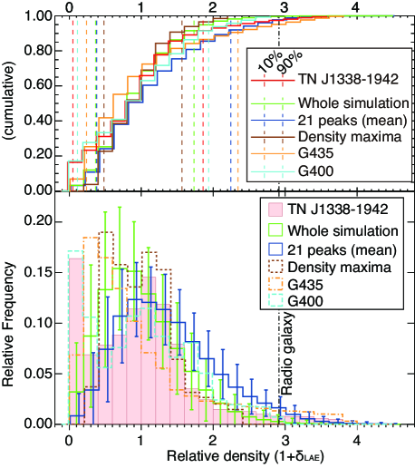
Figure 7: Comparison of the density distributions between the TNJ1338 field and the simulated map with various conditions for the simulation. The filled red histogram shows the observed density distribution of the TNJ1338 field (the same as in Fig. 5 left). The green outlined histogram is the density distribution for the whole simulation volume. The errors were estimated by computing the density distributions for 400 different Suprime-Cam-sized fields centred at random points, calculating the standard deviation for each density bin. The blue outline is the averaged distribution for the 21 fields centred at density peaks higher than the density measured at the radio galaxy position, and with $G$’s higher than that of the whole simulated map. The orange dot-dashed and the cyan dashed histograms are for the fields with the largest $G$ and the highest void fraction among the 21 fields, respectively (G435 and G400 fields). The brown dotted histogram is for the field around the highest-density peak over the whole map. The cumulative distributions are shown in the top panel, together with the 10- and 90-percentiles. The histograms are slightly shifted along the $x$ axis to improve the visibility. The large fractions of pixels in the highest- and the lowest-density bins cannot be simultaneously reproduced with the simulated density map within the errors. Although the high-density regions can be reproduced at the peak positions, the high volume fraction of the void regions is not seen around typical peaks. The G400 simulated field best reproduces both the large void fraction and the high density tail seen in the TNJ1338 field. However the peak of the histogram around the average density ($1+\delta_{\rm LAE}=1$) is not so high, and the high density tail is not so long, compared with those seen in the TNJ1338 field.

It is also important to check the size of field-to-field variations within the simulation volume. To do this, we first obtained density maps centred at random positions. We selected 100 positions in each of the four slices within the central $440\times 440\,h^{-2}\rm Mpc^{2}$, and made density maps within a FoV of Suprime-Cam centred at these 400 points. Then we calculated the standard deviation for each bin of the density distribution using the 400 maps. Fig. 7 shows that the observed density distribution, especially the density contrast within a single field, is very different from that for the simulated map as a whole. The volume fraction within the medium- to high-density ($1+\delta_{\rm LAE}\sim 1-3$) bins in the TNJ1338 field agrees with that obtained from the whole simulation volume, at $1\sigma$ level. On the other hand, the relative frequencies for the lowest- and the highest-density bins do not agree with those for the simulated map. This also suggests that such extreme overdensities / underdensities as we found observationally are quite rare in the simulation: the random sampling in the simulated map is unlikely to reproduce the unusual density distribution observed in our field. In fact, we found only 94 density peaks higher than that measured at the radio galaxy position, over the whole simulated map. Among the fields centred at the 94 peaks, only 21 has $G$’s higher than that of the whole simulated map (see §4.3.2). Since the TNJ1338 field has higher $G$ than the whole simulation (and the SXDS field), the number density of TNJ1338-like field is thought to be close to that of such high-$G$ fields. The number density is thus comparable to that of Coma-type protoclusters identified in the same simulation (58 protoclusters: chiang2013). The number (21 peaks) corresponds to number density of $6.4\times 10^{-8}\rm Mpc^{-3}$ in comoving units. This number density is also comparable to that of known bright radio sources at $z>2$ (see the section below). However, most of these peaks do not seem to reproduce the high density contrast seen in the TNJ1338 field. This suggests that high-density regions that host powerful radio galaxies associated with a giant Ly $\alpha$ nebulae, like our observed field, should be much rarer than this.

4.3.2 Density fields around the high-density peaks

Next we checked the density distributions around the 21 density peaks with large $G$’s found in the simulated map. In order to obtain the density distribution in the same manner as the observed data, we extracted the LAEs within a single Suprime-Cam FoV centred at the peak positions. Then we made the density maps in these fields, and calculated the density distributions using the grid points within the central $40\times 27.5\,h^{-2}\rm Mpc^{2}$, similarly to the analyses for the observed LAE sample. Fig. 7 also shows the average density distribution of the fields around the 21 density peaks, together with the errors. This average distribution is shifted toward higher density compared with the whole simulated map, smoothed along the density axis. However, the shape of the distribution does not significantly change: it agrees very closely with that of the whole map if we normalise the density with the average within these 21 fields, instead of the average of the whole simulated map. The distribution again seems to be different from the distribution in the TNJ1338 field, although the high-density tail is reproduced well. This implies that high-density regions just adjacent to the void regions, like we observed, are still much rarer than simple high-density peaks. For example, we can see that the field around the density maxima (normalised with the average within the same field) shows much narrower distribution than the observed one in the TNJ1338 field.

To further analyse the density distribution, we calculated the Gini coefficient for each map centred at the 21 high-density peaks. Fig. 5 shows the comparison of the Lorentz curves for the observed- and simulated density maps. The ordinate corresponds to the cumulative sum of the abscissa of the left panel, normalised with the total sum of the LAE surface density measured at each grid point. This shows that, while the density distribution of the SXDS field is well within the scatter of the simulated map, the distribution of the TNJ1338 field is far from the simulated ones, even from those around most of the density peaks. The possible exceptions are three peaks reproducing the $G\geq 0.4$. These three highest-$G$ peak has $G=0.435$, 0.403, and 0.400 (hereafter G435, G403, and G400 fields, respectively), which are fairly close to the observed $G$ in the TNJ1338 field. Of these three, two highest-$G$ fields (G435 and G403) does not have sufficiently high volume fraction of the void regions, and have only one peak between the average- and zero density, as seen in Fig. 7. The G400 field, in contrast, has exceptionally high void fraction ($\sim 15$ percent of the density cells are classified into the lowest density bin). This is the largest void fraction seen in the 94 peaks, which is still $\sim 1.5$ times higher than that in the field with the second largest void fraction (the second largest fraction was found in the G435 field). The G400 field has thus the density distribution closest to that of the TNJ1338 field among the whole simulated map. The peak density of G400 field is $1+\delta_{\rm LAE}=3.26$ when normalised with the average over the whole map, and 2.86 when normalised within the same FoV (see Table 4). The other two high-$G$ fields seems to be reproducing better than the G400 field in terms of the peak density, but the density distribution (e.g., the dynamic range and the void fraction) of the G400 field better reproduces the properties of TNJ1338 field.

Table 4: Statistics of the simulated density field

Field	Mean ${}^{a}$	Peak ${}^{b}$	Percentiles ${}^{b}$			$G$ ${}^{c}$
	$[h^{2}\rm Mpc^{-2}]$		10	50	90
G435	0.0409	3.87 (3.17)	0.24 (0.19)	0.71 (0.59)	2.35 (1.92)	0.435
G403	0.0613	2.77 (3.40)	0.24 (0.30)	0.72 (0.89)	2.21 (2.72)	0.403
G400	0.0570	2.86 (3.26)	0.11 (0.13)	0.97 (1.11)	1.94 (2.21)	0.400
Density maxima	0.1104	2.37 (5.24)	0.48 (1.07)	0.97 (2.15)	1.57 (3.46)	0.246
Whole map	0.0499	5.19	0.365	0.92	1.73	0.301

${}^{a}$Mean surface density over the field in comoving scale.

${}^{b}$In units of the relative density $(1+\delta_{\rm LAE})$ normalised with the average of the FoV of Suprime-Cam in the same field. Parenthesises show the densities normalised with the average of the whole simulated map.

${}^{c}$Gini coefficient of the density distribution.