Plasma dispersion in fractional-dimensional space

Abstract

The dielectric function for electron gas with parabolic energy bands is derived in a fractional dimensional space. The static response function shows a good dimensional dependence. The plasma frequencies are obtained from the roots of the dielectric functions. The plasma dispersion shows strong dimensional dependence. It is found that the plasma frequencies in the low dimensional systems are strongly dependent on the wave vector. It is weakly dependent in the three dimensional system and has a finite value at zero wave vector.

I Introduction

When the well width of a quantum well (QW) is extremely narrow and its barrier height that causes the in-plane confinement is infinite, the QW shows two-dimensional (2D) electronic and optical properties. The infinitely wide QW exhibits the three-dimensional (3D) bulk properties of the well materialMatos . The electronic and optical properties in a QW with finite barrier height and narrow well width show 3D behavior of the barrier material. It happens since the envelope functions for electrons and holes spread into the barrier region partially restoring the 3D characteristics of the system. On the other hand, the electronic and optical properties in a finite QW with sufficiently wide well width show 3D characteristics of the well material. Consequently the QW with finite well width and barrier height shows the fractional dimensional behavior which is somewhere in between 2D and 3D. This has been demonstrated by IshidaIshida in the calculation of plasma dispersion in a superlattice. The same behavior has also been demonstrated in the calculation of excitonJai and polaronSmondyrev ground state properties.

The anisotropic interactions in an anisotropic solid are treated as ones in an isotropic fractional dimensional space, where the dimension is determined by the degree of anisotropyHe . Thus only a single parameter known as the degree of dimensionality $(\alpha)$ is needed to describe the system. In the quantum well structures the width of the QW can also serve for determining $\alpha$ of the system. The fractional dimensional $\alpha D$ space is not Euclidean space, it is spectroscopic dimension which is observedBak . The $(\alpha$D) space is not a vector space and the coordinates in this space are termed as pseudo coordinatesStillinger .

The advantage of the $\alpha$D space approach over the conventional method for calculating different electronic and optical properties in the low dimensional systems is that it is easier to apply this method. For example, the $\alpha D$ space approach has been successfully employed to calculate exciton binding energy in QWs in an analytic methodHe1 ; Matos1 , while the conventional method needs involved numerical calculationsJai . Similarly the polaron properties in the $\alpha D$ space have been studied in a simple methodPolaron whereas the conventional method needs quite a bit of computational effortSmondyrev . The technique has also been used to study biexcitonsBiex1 ; Biex2 ; Biex3 , magnetoexcitonMagnet1 ; Magnet2 , exciton-exciton interactionExex , exciton-phonon interactionExph , Stark shift of exciton complexes in weak electric fieldStark , refractive indexTanguy , impurity and donor statesImp1 ; Harrison ; Imp2 , Pauli blocking effectPauli , exciton-phonon interactionExphn , exciton-polaron interactionExpol and magnetopolaronMagpol . The absorption spectra in a quantum wire shows the fractional dimensional space behavior with the dimension of the system lies between 1 and 3 depending on the size of the systemKarlsson .

Several properties of the charged boson system have been studied in the $\alpha D$ space using the Singwi-Tosi-Land-Sjölander (STLS) methodBoson . The Luttinger liquidCastelliani and the breakdown of Fermi liquid due to long range interactionWirefd in the fractional dimensional space with the dimension between 1 and 2 have been studied. In the fractional dimensional space the plasma frequencies in the long-wavelength limit have been derived from the real part of the dielectric function both in the quantum and classical limitsPanda . However, the full treatment of the dielectric function in the $\alpha D$ space for finding plasma frequency has not been carried out for Fermi gas. The present paper aims to fill up this gap and study the correlation energy.

II Dielectric function

In the $\alpha D$ space, the dielectric function with the wave vector $q$ and frequency $\omega$ of the external charge is defined asVignale

$$\epsilon_{\alpha D}(q,\omega)=1-v_{\alpha D}(q)\chi^{0}(q,\omega),$$ (1)

where $v_{\alpha D}(q)$ is the Fourier transform of Coulomb potential $e^{2}/\epsilon_{\infty}r$ in $\alpha$D space and $\chi^{0}_{\alpha D}(q,\omega)$ is the irreducible polarizability function. The expression for $v_{\alpha D}(q)$ is given asStillinger ,

$$v_{\alpha D}(q)=\frac{(4\pi)^{\frac{\alpha-1}{2}}\Gamma\biggl{(}\frac{\alpha-1}{2}\biggr{)}e^{2}}{q^{\alpha-1}},$$ (2)

where $\Gamma(x)$ is the Euler gamma function.

The irreducible polarizability function is defined asVignale

$$\chi^{0}_{\alpha D}(q,\omega)=\frac{2}{V_{\alpha D}}\sum_{\bf k}\frac{f({\bf k})-f({\bf k}+{\bf q})}{E_{\bf k}-E_{{\bf k}+{\bf q}}+\hbar\omega+i\epsilon},$$ (3)

where $f({\bf k})$ is the Fermi-Dirac distribution function, $V_{\alpha D}$ is the volume in $\alpha$D space and $\epsilon\rightarrow 0^{+}$. Rearranging Eq.(3), we find

$$\chi^{0}_{\alpha D}(q,\omega)=-\frac{2}{V_{\alpha D}}\sum_{\bf k}f({\bf k})\left[\frac{1}{E_{{\bf k}+{\bf q}}-E_{\bf k}-\hbar\omega-i\epsilon}+\frac{1}{E_{\bf k-{\bf q}}-E_{{\bf k}}+\hbar\omega+i\epsilon}\right]$$ (4)

We consider the zero-temperature limit and the parabolic energy dispersion, $E_{\bf k}=\hbar^{2}k^{2}/2m^{\ast}$ where $m^{\ast}$ is the effective mass of electron. The summation over k in the $\alpha D$ space approach is transferred into integration over $k$ and $\theta$ as

$$\sum_{\bf k}=\frac{V_{\alpha D}}{(2\pi)^{\alpha}}\frac{2\pi^{\frac{\alpha-1}{2}}}{\Gamma\biggl{(}\frac{\alpha-1}{2}\biggr{)}}\int^{k_{F}}_{0}k^{\alpha-1}dk\int^{\pi}_{0}\sin^{\alpha-2}\theta d\theta$$ (5)

In the $\alpha D$ space, the Fermi momentum $k_{F}$ is related to $r_{s}$ as

$$k_{F}r_{s}a_{B}=\beta_{\alpha},$$ (6)

where $a_{B}$ is the Bohr’s radius and $\beta_{\alpha}=[2^{d-1}\{\Gamma(1+d/2)\}^{2}]^{1/\alpha}$.

$$\chi^{0}_{\alpha D}(q,\omega) = -\frac{2^{2-\alpha}}{\pi^{\frac{\alpha+1}{2}}\Gamma\biggl{(}\frac{\alpha-1}{2}\biggr{)}}\int^{k_{F}}_{0}k^{\alpha-1}dk\int^{\pi}_{0}\sin^{\alpha-2}\theta d\theta$$ (7)

$$\left[\frac{1}{E_{q}+\hbar^{2}kq\cos\theta/m^{\ast}-\hbar\omega-i\epsilon}+\frac{1}{E_{q}-\hbar^{2}kq\cos\theta/m^{\ast}+\hbar\omega+i\epsilon}\right]$$

We have the identity

$$\frac{1}{x\pm i\epsilon}=P\biggl{[}\frac{1}{x}\biggr{]}\mp i\pi\delta(x),$$ (8)

where $P[1/x]$ is principal part of $1/x$ and $\delta(x)$ is the Dirac delta function.

II.1 Real part of the dielectric function

Using Eq.(8) in Eq.(7), we find

$$Re[\chi^{0}_{\alpha D}(q,\omega)] =-\frac{2^{2-\alpha}}{\pi^{\frac{\alpha+1}{2}}\Gamma\biggl{(}\frac{\alpha-1}{2}\biggr{)}}\int^{k_{F}}_{0}k^{\alpha-1}dk\int^{\pi}_{0}\sin^{\alpha-2}\theta d\theta$$ (9)

$$P\Biggl{[}\frac{1}{E_{q}+\hbar^{2}kq\cos\theta/m^{\ast}-\hbar\omega}+\frac{1}{E_{q}-\hbar^{2}kq\cos\theta/m^{\ast}+\hbar\omega}\Biggr{]}$$

The first and second integrals in Eq.(9) diverge when $\theta=\theta_{-}$ and $\theta=\theta_{+}$, respectively where $\theta_{\pm}=\arccos[m^{\ast}(\hbar\omega\pm E_{q})/\hbar^{2}kq$.

$$Re[\chi^{0}_{\alpha D}(q,\omega)] =-\frac{2^{2-\alpha}}{\pi^{\frac{\alpha+1}{2}}\Gamma\biggl{(}\frac{\alpha-1}{2}\biggr{)}}\int^{k_{F}}_{0}k^{\alpha-1}dk$$ (10)

$$\left[\int^{\pi}_{0}d\theta\frac{\left(\sin^{\alpha-2}\theta-\sin^{\alpha-2}\theta_{-}\right)}{E_{q}-\hbar\omega+\hbar^{2}kq\cos\theta/m^{\ast}}+\int^{\pi}_{0}d\theta\frac{\left(\sin^{\alpha-2}\theta-\sin^{\alpha-2}\theta_{+}\right)}{E_{q}+\hbar\omega-\hbar^{2}kq\cos\theta)/m^{\ast}}\right]$$

Carrying out the $\theta$ integration analytically, we find

$$Re[\chi^{0}_{\alpha D}(q,\omega)] = -\frac{2^{2-\alpha}}{\pi^{\frac{\alpha}{2}}\Gamma\biggl{(}\frac{\alpha}{2}\biggr{)}}\int^{k_{F}}_{0}k^{\alpha-1}dk$$ (11)

$$\Biggl{[}\frac{{{}_{2}F_{1}}\biggl{(}1,\frac{\alpha-1}{2},\alpha-1;\frac{2\hbar^{2}kq/m^{\ast}}{(E_{q}-\hbar\omega)-\hbar^{2}kq/m^{\ast}}\biggr{)}}{(E_{q}-\hbar\omega)-\hbar^{2}kq/m^{\ast}}+\frac{\pi\sin^{\alpha-2}\theta_{-}}{(E_{q}-\hbar\omega)^{2}-(\hbar^{2}kq/m^{\ast})^{2}}$$

$$+\frac{{{}_{2}F_{1}}\biggl{(}1,\frac{\alpha-1}{2},\alpha-1;\frac{2\hbar^{2}kq/m^{\ast}}{(E_{q}+\hbar\omega)+\hbar^{2}kq/m^{\ast}}\biggr{)}}{(E_{q}+\hbar\omega)+\hbar^{2}kq/m^{\ast}}+\frac{\pi\sin^{\alpha-2}\theta_{+}}{(E_{q}+\hbar\omega)^{2}-(\hbar^{2}kq/m^{\ast})^{2}}\Biggr{]},$$

where ${{}_{2}F_{1}}$ is the Gauss Hypergeometric function. The real part of the susceptibility $\chi^{0}(q,\omega)$ does not contain any divergent part in the range $\hbar v_{F}q-E_{q}<\hbar\omega<\hbar v_{F}q+E_{q}$. In this range the real part of the susceptibility is obtained as

$$Re[\chi^{0}_{\alpha D}(q,\omega)] =-\frac{2^{2-\alpha}k^{\alpha}_{F}}{\pi^{\frac{\alpha}{2}}\Gamma\biggl{(}\frac{\alpha-1}{2}\biggr{)}}\sum^{\infty}_{m=0}\frac{1}{(\alpha+2m)}(\hbar v_{F}q)^{2m}$$ (12)

$$\times\Biggl{[}\frac{1}{E_{q}-\hbar\omega)^{2m+1}}+\frac{1}{(E_{q}+\hbar\omega)^{2m+1}}\Biggr{]}\sum^{m}_{l=0}(-1)^{l}{m\choose l}\frac{\Gamma\biggl{(}\frac{\alpha+2l-2}{2}\biggr{)}}{\Gamma\biggl{(}\frac{\alpha+2l}{2}\biggr{)}}$$

II.2 Imaginary part of the dielectric function

The imaginary part of the irreducible polarizability function can be derived from Eq.(7) by using Eq.(8) as

$$Im[\chi^{0}_{\alpha D}(q,\omega)] = -\frac{2^{2-\alpha}}{\pi^{\frac{\alpha-1}{2}}\Gamma\biggl{(}\frac{\alpha-1}{2}\biggr{)}}\int^{k_{F}}_{0}k^{\alpha-1}dk\int^{\pi}_{0}\sin^{\alpha-2}\theta d\theta$$ (13)

$$\times\biggl{[}\delta\biggl{(}E_{q}+\hbar^{2}kq\cos\theta/m^{\ast}-\hbar\omega\biggr{)}-\delta\biggl{(}E_{q}-\hbar^{2}kq\cos\theta/m^{\ast}+\hbar\omega\biggr{)}\biggr{]}$$

Integrating over $\theta$, we find

$$Im[\chi^{0}_{\alpha D}(q,\omega)]=-\frac{2^{2-\alpha}m^{\ast}}{\pi^{\frac{\alpha-1}{2}}\Gamma\biggl{(}\frac{\alpha-1}{2}\biggr{)}} \biggl{[}\Theta(k_{F}-k_{-})\int^{k_{F}}_{k_{-}}k^{\alpha-2}dk\biggl{(}1-\frac{k^{2}_{-}}{k^{2}}\biggr{)}^{\frac{\alpha-3}{2}}$$ (14)

$$\times-\Theta(k_{F}-k_{+})\int^{k_{F}}_{k_{+}}k^{\alpha-2}dk\biggl{(}1-\frac{k^{2}_{+}}{k^{2}}\biggr{)}^{\frac{\alpha-3}{2}}\biggr{]}$$

where $k_{\pm}=\frac{m^{\ast}}{\hbar^{2}q}|\hbar\omega\pm E_{q}|$.

Performing the integration over $k$-space gives the result

$$Im[\chi^{0}_{\alpha D}(q,\omega)]=-\frac{2^{2-\alpha}m^{\ast}}{(\alpha-1)\pi^{\frac{\alpha-1}{2}}\Gamma\biggl{(}\frac{\alpha-1}{2}\biggr{)}\hbar^{2}q}\biggl{[}\Theta(k_{F}-k_{-})(k^{2}_{F}-k^{2}_{-})^{\frac{\alpha-1}{2}}-\Theta(k_{F}-k_{+})(k^{2}_{F}-k^{2}_{+})^{\frac{\alpha-1}{2}}\biggr{]}$$ (15)

II.3 Static response function and Plasma dispersion

The scaled static response function $F_{\alpha D}(q)=\chi^{(0)}_{\alpha D}(q,\omega\rightarrow 0)/\chi^{(0)}_{\alpha D}(0,\omega\rightarrow 0)$ is a measure of the number of excited states available to the system for vanishing excitation energy. Therefore $F_{\alpha D}(q,0)$ vanishes in the systems where there is a gap in the excitation spectrum. The calculated $F_{\alpha D}(q,0)$ for $\alpha=$1, 1.5, 2, 2.5 and 3 at $k_{F}=$0.5 a.u. and $m^{\ast}=m_{0}$ are shown in Fig.1. According to Eq.(6), the $r_{s}$ values corresponding to $k_{F}=$0.5 a.u. are $r_{s}$=1.57, 2.25, 2.8, 3.34 and 3.83 for $\alpha$=1, 1.5, 2, 2.5 and 3, respectively. The static response functions in integer dimensions 1D, 2D and 3D have been previously reportedVignale . There are singularities at $q=2k_{F}$ in all dimensions. In 1D there is a logarithm divergence. This singular behavior is responsible for Peirls instability which is the spontaneous formation of density wave at $q=2k_{F}$. In 1.5D the response function is weaker and there is a weak kink at $q=2k_{F}$. In 2D the kink at $q=2k_{F}$ is quite significant. As the dimension is increased, the kink decreases and the derivatives of the response functions for $2\leq\alpha\leq 3$ diverge at $q=2k_{F}$. The divergence in response function at $q=2k_{F}$ results in oscillations with periodicity 2$k_{F}$ in the Fourier transformation of $F_{\alpha D}(q,0)$. These are Friedel oscillations which are direct consequence of the existence of Fermi surface.

The plasmon frequency $\omega_{p}(q)$ can be obtained from the roots of $\epsilon_{\alpha D}(q,\omega)=0$ which gives the condition,

$$1-v_{\alpha D}(q)Re[\chi^{0}_{\alpha D}(q,\Omega_{\alpha D}(q))]=0$$ (16)

Since the analytic solution of this equation does not exist, we find $\Omega_{\alpha D}(q)$ by numerical method. The plasmon frequencies at $k_{F}$=0.5 a.u. for different $\alpha$ values and are shown in Fig.2 . The plasma frequency in 3DLindhard has got a finite value at $q=0$. The plasma frequencies for 2D agree with those of SternStern . The plasma frequency in 1D has been calculated following Das Sarma and HwangDasSarma . For other dimensions the plasma frequency plasma frequency vanishes at $q=0$. The condition for the existence of undamped plasma oscillations is the the plasma frequency $\Omega_{\alpha D}(q)$ needs to be higher than $\omega_{+}(q)=\hbar(2k_{F}q+q^{2})/2m^{\ast}$ which is the boundary frequency of the single particle regime. The plasma line and e-h line never intersect, but are tangential at $q_{c}$. For $q>q_{c}$, the dielectric function has no root and it is called Landau damping. The plasma frequency touches the boundary frequency of the single particle regime at $\omega_{+}=\hbar(2k_{F}q+q^{2})/2m^{\ast}$

In order to understand this effect, we evaluate the plasma frequency in the long-wavelength limit. In the long-wavelength limit $q\rightarrow 0$, $Im[\chi^{0}_{\alpha D}(q,\omega)]=0$. Taking $m=0$ and 1 in the $m$ summation in Eq.(12), we find

$$Re[\chi^{0}_{\alpha D}(q,\omega)]=-\frac{2^{1-\alpha}k^{\alpha}_{F}}{\pi^{\frac{\alpha}{2}}\Gamma\biggl{(}1+\frac{\alpha}{2}\biggr{)}}\Biggl{[}\frac{2E_{q}}{E^{2}_{q}-\hbar^{2}\omega^{2}}+\frac{2\hbar^{2}v^{2}_{F}q^{2}}{\alpha+2}\biggl{(}\frac{E^{3}_{q}+3E_{q}\hbar^{2}\omega^{2}}{(E^{2}_{q}-\hbar^{2}\omega^{2})^{3}}\biggr{)}\Biggr{]}$$ (17)

For $E_{q}<<\hbar\omega$, $(E^{2}_{q}-\hbar^{2}\omega^{2})^{-1}=-(1+E^{2}_{q}/\hbar^{2}\omega^{2})/\hbar^{2}\omega^{2}$ and $(E^{3}_{q}+3E_{q}\hbar^{2}\omega^{2})/(E^{2}_{q}-\hbar^{2}\omega^{2})^{3}=-3E_{q}/\hbar^{4}\omega^{4}$. Substituting these values in Eq.(17), we find

$$Re[\chi^{0}_{\alpha D}(q,\omega)]=\frac{2^{1-\alpha}q^{2}k^{\alpha}_{F}}{\pi^{\frac{\alpha}{2}}m^{\ast}\Gamma\biggl{(}1+\frac{\alpha}{2}\biggr{)}\omega^{2}}\left[1+\frac{E^{2}_{q}+3\hbar^{2}v^{2}_{F}q^{2}/(\alpha+2)}{\hbar^{2}\omega^{2}}\right]$$ (18)

Substituting Eq.(18) in Eq.(16), the long-wavelength plasma frequency $\Omega^{lw}_{\alpha D}(q)$ is obtained as

$$\Omega^{lw}_{\alpha D}(q)=\omega_{\alpha D}(q)\left[1+\frac{3v^{2}_{F}q^{2}}{2(\alpha+2)\omega^{2}_{\alpha D}}+\frac{\hbar^{2}q^{4}}{8m^{\ast}\omega^{2}_{\alpha D}}\right],$$ (19)

where the classical plasma frequency $\omega_{\alpha D}(q)$ is given byeqn

$$\omega_{\alpha D}=\sqrt{\frac{2^{2\alpha-2}\Gamma(1+\frac{\alpha}{2})\Gamma(\frac{\alpha-1}{2})e^{2}q^{3-\alpha}}{\sqrt{\pi}\epsilon_{\infty}m^{\ast}r^{\alpha}_{s}}}.$$ (20)

The dimensionless density parameter is related to the electron density $n_{\alpha D}$ aseqn

$$r_{s}=\Biggl{[}\frac{\Gamma(1+\frac{\alpha}{2})}{\pi^{\frac{\alpha}{2}}n_{\alpha D}}\Biggr{]}^{\frac{1}{\alpha}}.$$ (21)

We can easily understand the long-wavelength $q$-dependence in plasma frequency in Fig.1 by inspecting Eq.(20). The plasma frequency in 3D system is nonzero at $q=0$ as it independent of $q$ vector. For $\alpha<3$, the plasma frequency vanishes at $q=0$.

III Conclusion

The dielectric function for electron gas in the fractional dimensional space has been derived in the RPA. Using the irreducible susceptibilities the static response functions for different $\alpha$ values have been calculated. The static response functions show derivative divergence for all dimensions except for 1D system where there is a logarithm singularity. However, the response function for 1.5D electron gas is weak. The plasma dispersion has been found from the root of the dielectric function. The plasma frequency for low dimensional systems vanishes at $q=0$. It gradually approaches towards bulk value when $\alpha$ increases. EricssonPlasma2D experimentally verified the plasma frequencies in a wide QW. Similarly the present results require experimental verification in a suitable well which shows fractional dimensional behavior. In future we are working on local field correction on the dielectric function and plasma frequency using the STLS method.

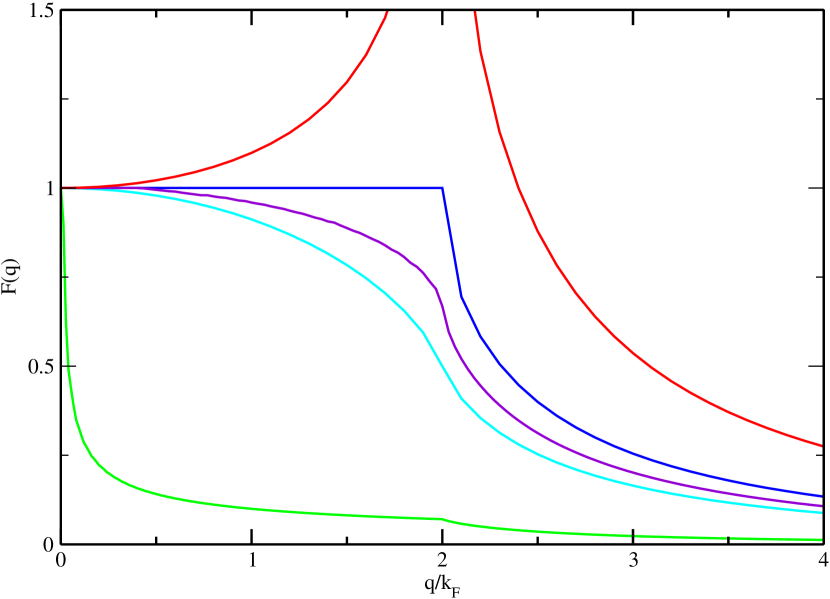
Figure 1: Static response functions in fractional dimensions as a function of wave vector. Here $k_{F}$=0.5 a.u. and $m^{\ast}=m_{0}$. Different color lines are denoted as $\alpha=$ 1 (red line), 1.5 (green line), 2 (blue line), 2.5 (violet line) and 3 (cyan line).

Figure 2: Plasma dispersion in fractional dimensions in several dimensions. Here $k_{F}$=0.5 a.u. and $m^{\ast}=m_{0}$. The black dot-dashed line represents the boundary of the single particle regime. Different color lines correspond to different dimensions as in Fig.1. Plasma frequencies are denoted by solid lines while plasma frequencies at long-wavelength limit are denoted by dashed lines.

References

• (1) A. Matos-Abiague, Phys. Rev. B65, 165321 (2002)
• (2) H. Ishida, J. Phys. Soc. Japan, 55, 4396 (1986)
• (3) A. Thilagam and J. Singh, Phys. Rev. B49, 13583 (1994)
• (4) M. A. Smondyrev, B. Gerlach and M. O. Dzero, Phys. Rev. B 62, 16692 (2000)
• (5) X. -F. He, Solid State Commun. 75, 111 (1990)
• (6) Z. Bak, Phys. Rev. B68, 64511 (2003)
• (7) F. H. Stillinger, J. Math. Phys. 18, 1224 (1977)
• (8) X. -F. He, Phys. Rev. B43, 2063 (1991)
• (9) A. Matos-Abiague, L. E. Oliveira and M. de Dios-Leyve, Phys. Rev. B58, 4072 (1998)
• (10) A. Matos-Abiague, J. Phys.: Condens. Matter 14, 4543 (2002)
• (11) A. Thilagam, Phys. Rev. B55, 7804 (1997)
• (12) D. Birkedal, J. Singh, V. G. Lyssenko, J. Erland and J. M. Hvam, Phys. Rev. Lett. 76, 672 (1996)
• (13) V. Mizeikis, D. Birkedal, W. Longebein, V. G. Lyssenko and J. M. Hvam, Phys. Rev. B55, 5284 (1997)
• (14) Q. X. Zhao, B. Monemar, P. O. Holtz, M. Wilander, B. O. Fimland and K. Johannessen, Phys. Rev. B50, 4476 (1994)
• (15) E. Reyes-Gomez, A. Matos-Abiague, C. A. Perdomo-Leiva, M. de Dios-Leyva and L. E. Oliveira, Phys. Rev. B61, 13104
• (16) A. Thilagam, Phys. Rev. B63, 45321 (2001)
• (17) A.Thilagam, Phys. Rev. B 56, 9798 (1997)
• (18) A. Thilagam, Phys. Rev. B56, 4665 (1997)
• (19) C. Tanguy, P. Lefevbre, H. Mathieu and R. J Elliot, J. Appl. Phys. 82, 798 (1997)
• (20) A. Matos-Abiague, L. E. Oliveira and M. de Dios-Leyva, Physica B296, 342 (2001)
• (21) J. Kundrotas, A. Cerskus, S. Asmontas, G. Valusis, B. Sherliker, M. P. Halsell, M. J. Steer, E. Johannessen and P. Harrison, Phys. Rev. B72, 255322 (2005)
• (22) I. D. Mikhailov, F. J. Betancur, R. A. Escorcia and J. Eierra-Ortega, Phys. Rev. B67, 115317 (2003)
• (23) A. Thilagam, Phys. Rev. B59, 3027 (1999)
• (24) A. Thilagam, Phys. Rev. B56, 9797 (1997)
• (25) A. Thilagam and A. Matos-Abiague, J. Phys.: Condens. Matter 16, 3981 (2004)
• (26) T. M. Rusin and J. Kossut, Phys. Rev. B56, 4687 (1997)
• (27) K. F. Karlsson, M. -A. Dupertuis, H. Weman and E. Kapon, Phys. Rev. B70, 153306 (2004)
• (28) S, Panda and B. K. Panda, Eur. Phys. J. B
• (29) C. D. Castelliani, C. Di Castro and W. Metzner, Phys. Rev. Lett. 72, 316 (1994)
• (30) P. -A. Bares and X. -G. Wen, Phys. Rev. B48, 8636 (1993)
• (31) S. Panda and B. K. Panda, J. Phys.:Condens. matter 20, 485201 (2008)
• (32) G. F. Giuliani and G. Vignale (Cambridge university press, New York, 2005)
• (33) J. Lindhard, K. Danske Vidensk. Selsk. Mat.-Fys. Meddr. 28, No.8 (1954)
• (34) F. Stern, Phys. Rev. Lett. 18, 546 (1967)
• (35) S. Das Sarma and E. H. Hwang, Phys. B 44, 1936 (1996)
• (36) Standard expression in literature is $\omega_{\alpha D}=\sqrt{(4\pi)^{{{\alpha-1}\over 2}}\Gamma({{\alpha-1}\over 2})e^{2}n_{\alpha D}q^{3-\alpha}/\epsilon_{\infty}m^{\ast}}$, where high-frequency dielectric constant $\epsilon_{\infty}$ is taken unity.
• (37) M. A. Ericsson, A. Pinczuk, B. S. Dennis, C. F. Hirjibehedin, S. H. Simon, L. N. Pfeiffer and K. W. West, Physica E 6, 165 (2000), C. F. Hirjibehedin, A. Pinczuk, B. S. Dennis, L. N. Pfeiffer and K. W. West, Phys. Rev. B. 65, 161309 (2002)
Refer to caption