Scalar boundary value problems on junctions
of thin rods and plates.
I. Asymptotic analysis and error estimates

Abstract

We derive asymptotic formulas for the solutions of the mixed boundary value problem for the Poisson equation on the union of a thin cylindrical plate and several thin cylindrical rods. One of the ends of each rod is set into a hole in the plate and the other one is supplied with the Dirichlet condition. The Neumann conditions are imposed on the whole remaining part of the boundary. Elements of the junction are assumed to have contrasting properties so that the small parameter, i.e. the relative thickness, appears in the differential equation, too, while the asymptotic structures crucially depend on the contrastness ratio. Asymptotic error estimates are derived in anisotropic weighted Sobolev norms.

Keywords: junction of thin plate and rods, asymptotic analysis, dimension reduction, boundary layers, error estimates.

MSC: 35B40, 35C20, 74K30

1 Introduction

1.1 Formulation of the problem

Let $\mathbb{\omega}_{0}$ and $\mathbb{\omega}_{j\text{ }}$be domains in the plane $\mathbb{R}^{2}$ bounded by smooth simple closed contours $\partial\mathbb{\omega}_{p};$ here and everywhere in the paper $j=1,....J$ and $p=0,....J$, while $J\in\mathbb{N}=\{1,2,3,...\}.$ Moreover, the summation over $j=1,...,J$ will be further denoted by $\sum_{j}$. The closures $\overline{\mathbb{\omega}}_{p}=\mathbb{\omega}_{p\text{ }}\cup\partial\mathbb{\omega}_{p}$ are compact and the origin of the Cartesian coordinates $y=(y_{1},y_{2})$ belongs to $\mathbb{\omega}_{j}.$ We fix some points $P^{1},....,P^{{J}}$ inside $\mathbb{\omega}_{0}$, $P^{j}\neq P^{k}$ for $j\neq k,$ and introduce the thin plate

$$\Omega_{0}(h)=\{x=(y,z)\in\mathbb{R}^{3}:y\in\mathbb{\omega}_{0},\text{ }\zeta:=h^{-1}z\in(0,1)\}$$ (1.1)

and the thin rods

$$\Omega_{j}(h)=\{x:\eta^{j}=:h^{-1}(y-P^{j})\in\mathbb{\omega}_{j},\text{ \ }z\in(0,l_{j})\}$$ (1.2)

where $h\in(0,h_{0}]$ is a small parameter and $l_{1},...,l_{{J}}$ are fixed positive numbers. The bound $h_{0}>0$ is chosen such that the closures of the small sets $\mathbb{\omega}_{j}^{h}=\{y:\eta^{j}\in\mathbb{\omega}_{j}\}$ are contained in the domain $\mathbb{\omega}_{0}$ for all $h\in(0,h_{0}]$. In the sequel, if necessary, we may diminish this bound but always keep the notation $h_{0}.$

The junction

$$\Xi(h)=\Omega_{\bullet}(h)\cup\Omega_{1}(h)\cup....\cup\Omega_{J}(h)$$ (1.3)

of the plate and rods, see fig. 1,a, involves the intact rods (1.2) but the plate $\Omega_{\bullet}(h)$ with cylindrical holes (column sockets), fig. 1,b,

$$\Omega_{\bullet}(h)=\mathbb{\omega}_{\bullet}(h)\times(0,h),\quad\mathbb{\omega}_{\bullet}(h)=\mathbb{\omega}_{0}\mathbb{\diagdown}(\overline{\mathbb{\omega}_{1}^{h}}\cup.....\cup\overline{\mathbb{\omega}_{{J}}^{h}}).$$ (1.4)

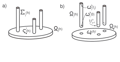
Figure 1: The junction (a) and its elements (b). The Dirichlet zones are shaded.

The bases of the intact (1.1) and perforated (1.4) plates are denoted respectively by

$$\varsigma_{0}^{i}(h)=\{x:y\in\mathbb{\omega}_{0},\ z=ih\},\ \ \ \varsigma_{\bullet}^{i}(h)=\{x:y\in\mathbb{\omega}_{\bullet},\ z=ih\},\ \ i=0,1,$$ (1.5)

and the common lateral side by $\upsilon_{0}(h)=\partial\mathbb{\omega}_{0}\times(0,h).$ The ends of the rod (1.2) are

$$\mathbb{\omega}_{j}^{h}(0)=\mathbb{\omega}_{j}^{h}\times\{0\},\ \ \mathbb{\omega}_{j}^{h}(l_{j})=\mathbb{\omega}_{j}^{h}\times\{l_{j}\}$$ (1.6)

while the lateral side of the rod is divided into two parts

$$\Sigma_{j}(h)=\partial\mathbb{\omega}_{j}^{h}\times(h,l_{j}),\ \ \mathbb{\upsilon}_{j}^{h}=\partial\mathbb{\omega}_{j}^{h}\times(0,h),$$ (1.7)

the latter being the contact zone of $\Omega_{\bullet}(h)$ and $\Omega_{j}(h).$ These sets are indicated in fig. 1.

In the junction (1.3) we consider the Poisson equations

$$-\Delta_{x}u_{0}(h,x) =f_{0}(h,x),\ \ \ x\in\Omega_{\bullet}(h),$$ (1.8)

$$-\gamma_{j}(h)\Delta_{x}u_{j}(h,x) =f_{j}(h,x),\ \ \ x\in\Omega_{j}(h),$$ (1.9)

equipped with the Neumann and Dirichlet boundary conditions

$$\partial_{\nu}u_{0}(h,x) =0,\ \ \ \ x\in\Sigma_{\bullet}(h)=\varsigma_{\bullet}^{0}(h)\cup\varsigma_{\bullet}^{1}(h)\cup\mathbb{\upsilon}_{0}(h)$$ (1.10)

$$\gamma_{j}(h)\partial_{\nu}u_{j}(h,x) =0,\ \ \ x\in\Sigma_{j}(h)\cup\mathbb{\omega}_{j}^{h}(0),$$ (1.11)

$$u_{j}(h,x) =0,\ \ \ x\in\mathbb{\omega}_{j}^{h}(l_{j}),$$ (1.12)

together with the transmission conditions

$$u_{0}(h,x) =u_{j}(h,x),\ \ \ \ x\in\mathbb{\upsilon}_{j}^{h},$$ (1.13)

$$\partial_{\nu}u_{0}(h,x) =\gamma_{j}(h)\partial_{\nu}u_{j}(h,x),\ \ \ x\in\mathbb{\upsilon}_{j}^{h}.$$ (1.14)

Here, $\Delta_{x}$ is the Laplace operator in $x=(y,z)=(x_{1},x_{2},x_{3}),$ $u_{0}$ and $u_{j}$ are restrictions of the function $u$ on the subdomains $\Omega_{\bullet}(h)$ and $\Omega_{j}(h),$ $f_{0}=f|_{\Omega_{\bullet}(h)}$ and $f_{j}=f|_{\Omega_{j}(h)}$ having the similar meaning, $\partial_{\nu}=\nu\cdot\nabla_{x}$ is the directional derivative, while $\nabla_{x}=\operatorname{grad}$ and $\nu$ is the unit vector of the outward normal on the surfaces $\partial\overline{\Xi(h)}$ and $\partial\Omega_{j}(h).$ Notice that $\partial_{\nu}=\partial_{z}=\partial/\partial z\text{ \ \ on }\varsigma_{0}^{1}(h)\text{ \ and }\partial_{\nu}=-\partial_{z}\text{\ \ on }\varsigma_{0}^{0}(h).$

The coefficient

$$\gamma_{j}(h)=\gamma_{j}h^{-\alpha}>0$$ (1.15)

in (1.9), (1.11) and (1.14) describes contrasting properties of elements in the junction (1.3). Namely, regarding $u(h,x)$ as a stationary temperature field in $\Xi(h),$ we obtain a homogeneous body in the case $\alpha=0,$ $\gamma_{j}=1$ but in the case $\alpha>0$ the conductivity of the rods $\Omega_{j}(h)$ is much bigger than of the plate $\Omega_{\bullet}(h).$ In what follows we deal with two typical cases

$$\alpha=0\text{ \ and \ }\alpha=1.$$ (1.16)

As mentioned above, the first case may be attributed to the homogeneous junction. In the second case the integral conductivity of the plate vertical segment $(0,h)$ and of the rod cross-section $\omega_{j}^{h},$ that are $h$ and $\gamma_{j}(h)\operatorname*{mes}_{2}\omega_{j}^{h}=h\gamma_{j}\operatorname*{mes}_{2}\omega_{j}$ respectively, become of the same order in $h.$ The latter complicates both, the asymptotic ansätze for the solution $u(h,x)$ of problem and the asymptotic procedure. To construct the asymptotics as $h\rightarrow+0$ and to justify it by deriving error estimates are just the main goal of the paper.

The variational formulation of problem (1.8)-(1.14) reads: to find a function $u\in H_{0}^{1}(\Xi(h);\Gamma(h))$ satisfying the integral identity [24]

$$a(u,v;\Xi(h))=(f,v)_{\Xi(h)}\ \ \ \forall v\in H_{0}^{1}(\Xi(h);\Gamma(h)).$$ (1.17)

Here, $H_{0}^{1}(\Xi(h);\Gamma(h))$ is a subspace of functions in the Sobolev space $H^{1}(\Xi(h))$ which meet the Dirichlet condition (1.12) and $(\ ,\ )_{\Xi(h)}$ is the natural scalar product in the Lebesgue space $L^{2}(\Xi(h)).$ Furthermore,

$$a(u,v;\Xi(h))=(\nabla_{x}u_{0},\nabla_{x}v_{0})_{\Omega_{\bullet}(h)}+{\textstyle\sum\nolimits_{j}}\gamma_{j}(h)(\nabla_{x}u_{j},\nabla_{x}v_{j})_{\Omega_{j}(h)}$$ (1.18)

and $\Gamma(h)$ is the union of the upper ends $\omega_{j}^{h}(l_{j})$ of the rods. As usual, the integral identity is obtained by multiplying the equations (1.8), (1.9) by test functions $v_{0},$ $v_{j}$ and integrating by parts in $\Omega_{\bullet}(h),$ $\Omega_{j}(h)$ while taking into account the boundary (1.10), (1.11) and transmission (1.14) conditions for $u$ and also the stable conditions (1.12), (1.13), absorbed in the space $H_{0}^{1}(\Xi(h);\Gamma(h))$ and therefore given to the test function $v.$

1.2 Asymptotic analysis of junctions

Bodies made of thin elements are met everywhere in our daily life; one may think about miscellaneous mechanisms and their details, bridges and wheels with spokes, chairs and tables, etc. Even flora and fauna give examples of all kinds of such junctions. Mathematical studies of junctions of domains with different limit dimensions have provided several approaches diversified by levels of rigor and ways to formulate results.

Junctions of type ”massive body/thin rods”, fig 2,a, were inspected from all sides, most intensely among other types. Asymptotic formulas together with error estimates for fields of various physical nature are obtained and hybrid variational-asymptotic models are derived, see, e.g., the papers [18, 2, 1, 21, 34, 10, 40] for scalar differential equations and [5, 6, 27, 9, 35, 22, 23, 39, 41, 43] for elasticity and other systems; vast citation lists can also be found in the monograph [26, 20] and the review paper [42].

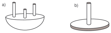
Figure 2: The juncton of a massive body and rods (a). The junction of a mushroom type (b). The Dirichlet zones are shaded.

Junction of thin plates and rods have been considered as well, see [38, 12, 13] for scalar equations and [14, 15, 11, 3, 4] for elasticity. However, the known results, cf. [12, 13], for scalar equations concern only the case  $J=1,$ see fig. 2,b, and, more importantly, the lateral side $\upsilon_{0}(h)$ of the plate $\Omega_{0}(h)$ used to be endowed with the Dirichlet condition, that is

$$-\partial_{z}u_{0}(h,y,0) =\partial_{z}u_{0}(h,y,h)=0,\ \ \ y\in\omega_{\bullet}(h),$$ (1.19)

$$u_{0}(h,y,z) =0,\ \ \ (y,z)\in\upsilon_{0}(h):=\partial\omega_{0}\times(0,h),$$

instead of (1.10). In elasticity the Dirichlet condition means that the edge of the ”mushroom cap” in fig. 2,b, must be clamped as well as the lower part of ”mushroom leg”. Besides, for the stationary heat equation under consideration, the constant (null) temperature in problem (1.8), (1.9), (1.19), (1.11)-(1.14) is maintained not only at the ”soles” of the rods but on the lateral side of the plate, too. Evidently, both cases (1.10) and (1.19) may occur in practice and in the sequel we state the scalar boundary value problem on junction (1.3) just in the same way as for the above-mentioned junctions ”massive body/thin rods” in [21, 34, 40], [20] and others.

Another departure from results obtained in [12, 13] and other publications consists in the derivation of estimates of the asymptotic remainders while the previous treatment asserts convergence results without estimating the convergence rate. For a spatial junction of type ”thin plate/thin rods” formulation of asymptotic formulas is a matter of principle because one of the limit problem is planar and, as discovered in [16] (see also [17], [30, Ch.2, 4, 5]) a singular perturbation of the boundary may lead to the rational dependence on $\ln h$ of asymptotic terms expansions. This indeed happens in the case $\alpha=1$ (cf. Section 3.1) due to the appearance of logarithm in the fundamental solution of the Laplacian in $\mathbb{R}^{2}.$ Asymptotic series in $|\ln h|^{-1},$ of course, are available but, being convergent, they however provide rather rough proximity of order $|\ln h|^{-N}$ while taking into account the rational dependence brings order $h^{\delta},$ $\delta>0.$

The case $\alpha=0$ generates another effect: asymptotic expansions of the solution $u(h,x)$ of problem (1.8)-(1.14) gain terms of order $h^{-1}$ even for a smooth uniformly bounded right-hand sides $f_{p}(h,x)$ in the differential equations, see Section 3.3. Moreover the next terms becomes linear functions in $\ln h,$ i.e., also grow when $h\rightarrow+0.$ These facts make a formulation of the asymptotic decomposition as a convergent result doubtful, cf. a pour formulation in Section 4.6.

We emphasize that both the above-mentioned peculiarities of the asymptotic behavior of the solution $u(h,x)$ vanish if the boundary conditions (1.10) are replaced with (1.19). In particular all solutions with logarithmic singularities we use below, disappear from the analysis of main asymptotic terms and the convergence theorems of [12, 13].

1.3 The asymptotic method

Asymptotic expansions of solutions to elliptic boundary value problems in domains with singularly perturbed boundary can be constructed by means of two, certainly equivalent methods, namely the method of matched asymptotic expansions and the method of compound asymptotic expansions; we refer, respectively, to the monographs [50, 17] and [30, 20], these lists could be elongated quite much, where a complete description of the methods is given and, furthermore, the equivalency is clarified in [30, Ch.2]. Previous studies of junctions of type ”massive body/thin rods” were mainly based on the method of compound expansion because just this method elucidates boundary layer effects in the vicinity of the juncture zones. These effects are described by boundary value problems in the union of a semi-cylinder and a half-space $\mathbb{R}_{+}^{3}$ while the intrinsic power-law decay of their solutions makes the method of compound expansions much more preferable.

For the homogeneous ($\alpha=0$) junction $\Xi(h)$ of thin plate and rods the boundary layer terms are solutions of the Neumann problem in the union $\Xi_{j}$ of the semi-cylinder $Q_{j}$ and the perforated layer $\Lambda_{j},$ see (2.32). Moreover, the contrasting properties of the junction elements, that is $\alpha=1$ in (1.15), split the problem in $\Xi_{j}$ into two independent problems in $Q_{j}$ and $\Lambda_{j},$ cf. Sections 2.4 and 3.3. Unfortunately, the solutions of the problems in $Q_{j}$ and $\Lambda_{j}$ no longer get a decay at infinity in the layer but quite the contrary they gain a logarithmic growth. The latter brings a complication into the application of compound expansions (cf. [30, Ch.2]) and that is why in the paper we use the method of matched asymptotic expansions. Namely we construct outer and inner expansions which, respectively, involve singular solutions of the limit problems in $\omega_{0}$ and growing solutions of the limit problems in $\Xi_{j}$ and $\Lambda_{j}.$ The expansions acquire a family of free constants, actually $A_{0}$ and $A_{1},...,A_{J}$ in Proposition 1, but the standard matching procedure, which equalizes main asymptotic terms of the outer expansions as $x\rightarrow P^{j}$ and main asymptotic terms of the inner expansions at infinite, results into a system of linear algebraic equations which allow us to determine the free constants. It should be stressed that every particularity in the asymptotic behavior of the solution $u(h,x)$ originates in the structure of the algebraic system which, in its turn, is totally predetermined by the general attributes of the junction.

We also point out that the choice of the method of matched asymptotic expansions is prompted by a goal of our proceeding paper, namely to create an asymptotic variational model of a junction of type ”thin plate/thin rods” which involves certain self-adjoint extensions of differential operators of the limit problems. Indeed, it is the paper [36] where an intrinsic relationship of the method and the technique of self-adjoint extensions was revealed for elliptic problem in singularly perturbed domains. We emphasize that in [29] an application of self-adjoint extensions for junctions of domains with different limit dimensions was formulated as an open question; however, only junction of type ”massive body/thin rods” have been examined in this way, cf. [40, 39, 41].

Once asymptotics is clarified, we use a construction of a global approximation on involving cut-off functions with ”overlapping supports” (see [30, Ch.2]) which helps to satisfy all boundary and transmission conditions and to diminish residuals left in the differential equations (1.8) and (1.9). After applying a priori estimates of solutions to the variational problem (1.17), we finally cleanse the used intermediate approximate solution from those cut-off functions and formulate error estimates on each element of the junction. The latter explains soundly convergence theorems and will be used to justify the above-mentioned asymptotic-variational models.

1.4 Architecture of the paper

In Section 2 we derive and analyze different limit problems whose solutions are used in Section 3 in order to construct the formal asymptotics of the solution $u(h,x)$ to the original problem in the junction cases (1.16). We also indicate in Sections 3.2 and 3.4 significant simplifications occurring due to the restriction $J=1$ and the Dirichlet boundary condition on the plate lateral side $\upsilon_{0}(h)=\partial\omega_{0}\times(0,h).$ A justification of the general asymptotic procedures in Section 3.1 for $\alpha=1$ and in Section 3.3 for $\alpha=0$ is given in Section 4 which starts with derivation of several weighted estimates summarized in Theorem 9. After listing some necessary restrictions on the problem data in Section 4.3, we prove in Section 4.5 Theorem 12 for $\alpha=1$ and in Section 4.6 Theorem 15 for $\alpha=0$ which provide sharp estimates of the remainders. These estimates also allow us to conclude in Corollaries 13 and 16 evident assertions on convergence of the solution components $u_{0}(h,x)$ and $u_{j}(h,x)$ as $h\rightarrow+0.$

Finally in Section 5 we outline available generalizations in our present formulation of the problem.

2 Limit problems

We here discuss the limit problems whose solutions form the asymptotic expansions of the solution $u(h,x)$ of problem (1.8)-(1.14) in the junction (1.3) specified in (1.15) and (1.16). The first couple of the limit problems for rods and plates is rather standard, cf. [30, 20, 45, 31] and others, and we outline them briefly while paying the most attention to singular solutions of the Neumann problem in $\omega_{0}$ which play an important role in the outer expansion in the plate $\Omega_{\bullet}(h).$ Other limit problems appear in the union of a layer and a semi-cylinder or in a perforated layer, cf. fig. 3, and are intended to describe the inner expansions in the vicinity of the junction zones. These problems and the decompositions of their solutions are studied in Section 2.3 and 2.4 in detail.

2.1 The limit problems for the rods

We assume that the right-hand side of the differential equation (1.9) in the rod $\Omega_{j}(h)$ takes the form

$$f_{j}(h,x)=h^{-1-\alpha}f_{j}^{\bot}(\eta^{j},z)+h^{-\alpha}f_{j}^{0}(z)+\widetilde{f}_{j}(h,x),$$ (2.1)

where $f_{j}^{\bot}$ and $f_{j}^{0}$ are some functions on $\Omega_{j}(1)=\omega_{j}\times(0,l_{j})$ and $(0,l_{j}),$ respectively, while

$$\langle{f^{\bot}}\rangle_{j}(z):=\int_{\omega_{j}}f_{j}^{\bot}(\eta,z)d\eta=0,\ \ \ z\in(0,l_{j}).$$ (2.2)

In this section we suppose that $f_{j}^{\bot}$ and $f_{j}^{0}$ are smooth but a necessary restriction on their smoothness as well as a smallness of the remainder $\widetilde{f}_{j}$ will be formulated in Section 4.2.

Taking (2.1) and (1.15) into account we readily accept the asymptotic ansatz

$$u_{j}(h,x)=U_{j}^{0}(z)+hU_{j}^{1}(\eta^{j},z)+h^{2}U_{j}^{2}(\eta^{j},z)+...$$ (2.3)

Here and in what follows, dots stand for low order terms, inessential for our formal asymptotic analysis performed in Section 2. Inserting (2.3) and (2.1) into (1.9) and (1.11) we derive the recurrent sequence of the Neumann problems in the cross-section $\omega_{j}\ni\eta^{j}$ with the parameter $z\in(0,l_{j}),$

$$-\gamma_{j}\Delta_{\eta}U_{j}^{k}(\eta^{j},z)=F_{j}^{k}(\eta^{j},z),\ \ \ \eta^{j}\in\omega_{j},\ \ \ \ \ \ \ \ \gamma_{j}\partial_{\nu(\eta)}U_{j}^{k}(\eta^{j},z)=0,\ \ \ \eta^{j}\in\partial\omega_{j},$$ (2.4)

where $k=0,1,2$ and

$$F_{j}^{0}=0,\ F_{j}^{1}(\eta^{j},z)=f_{j}^{\bot}(\eta^{j},z),\ F_{j}^{2}(\eta^{j},z)=f_{j}^{0}(z)-\gamma_{j}\partial_{z}^{2}U_{j}^{-1}(z).$$

Clearly, relations (2.4) with $k=0$ are fulfilled. The problem (2.4) with $k=1$ has a solution due to the orthogonality condition (2.2) and this solution can be subject to the orthogonality conditions $\langle{U_{j}^{1}}\rangle_{j}(z)=0$. Finally, the problem (2.4) with $k=2$ becomes solvable provided

$$-\gamma_{j}|\omega_{j}|\partial_{z}^{2}U_{j}^{0}(z)=|\omega_{j}|f_{j}^{0}(z),\ \ \ z\in(0,l_{j}),$$ (2.5)

where the factor $|\omega_{j}|=\operatorname*{mes}_{2}\omega_{j},$ the area of the rod cross-section, appears after integration of $F_{j}^{2}(\eta^{j},z)$.

We supply the ordinary differential equation (2.5) with the condition

$$U_{j}^{c}(l_{j})=0$$ (2.6)

inherited from the Dirichlet condition (1.12). The other condition at the point $z=0$ which closes the limit problem for the rod, depends on the exponent $\alpha$ in (1.15) and we will find it in Section 3 only.

2.2 The limit problem for the plate

Similarly to (2.1)-(2.3), we set

$$f_{0}(h,x) =h^{-1}f_{0}^{\bot}(y,\zeta)+f_{0}^{0}(y)+\widetilde{f}_{0}(h,y),$$ (2.7)

$$\langle f^{\bot}_{0}\rangle(\zeta):= \int_{0}^{1}f_{0}^{\bot}(y,\zeta)d\zeta=0,\ \ \ y\in\omega_{0},$$ (2.8)

$$u_{0}(h,x) =U_{0}^{0}(y)+hU_{0}^{1}(y,\zeta)+h^{2}U_{0}^{2}(y,\zeta)+...$$ (2.9)

We insert the asymptotic ansätze (2.9) and (2.7) into the equation (1.8) in the perforated plate (1.4) as well as into the boundary conditions (1.10) at its bases $\varsigma_{\bullet}^{0}(h)$ and $\varsigma_{\bullet}^{1}(h),$ see (1.5). In this way we obtain a recurrent sequence of differential equations in the fast variable $\zeta=h^{-1}z\in(0,1)$ with the Neumann conditions at $\zeta=0$ and $\zeta=1.$ Owing to the orthogonality condition (2.8) we solve the problem

$$-\partial_{\zeta}^{2}U_{0}^{k}(y,\zeta)=F_{0}^{k}(y,\zeta),\ \ \ \zeta\in(0,1),\ \ \ \ \ \ \partial_{\zeta}U_{0}^{k}(y,0)=\partial_{\zeta}U_{0}^{k}(y,1)=0$$ (2.10)

with the index $k=1$ and the right-hand side $F_{0}^{1}$ from the list

$$F_{0}^{0}=0,\ F_{0}^{1}(y,\zeta)=f_{0}^{\bot}(y,\zeta),\ F_{0}^{2}(y,\zeta)=f_{0}^{0}(y)-\Delta_{y}U_{0}^{-1}(y).$$

Since this solution is defined up to an additive constant in $\zeta,$ we can satisfy the natural requirement $\langle U^{1}_{0}\rangle(\zeta)=0$. Noting that relation (2.10) with $k=-1$ is obviously met, we observe that the problem (2.10) with $k=1$ gets a solution if and only if

$$-\Delta_{y}U_{0}^{0}(y)=f_{0}^{0}(y),\ \ \ y\in\omega_{0}.$$ (2.11)

By virtue of the Neumann boundary condition (1.10) at the lateral side $\upsilon_{0}(h)$ of the plate, we impose

$$\partial_{\nu}U_{0}^{0}(y)=0,\ \ y\in\partial\omega_{0},$$ (2.12)

and regard (2.11), (2.12) as the limit problem for the plate $\Omega_{\bullet}(h).$

In contrast to the limit problems for the rods $\Omega_{j}(h)$ which involve the Dirichlet conditions (2.6) and hence are uniquely solvable, problem (2.11), (2.12) has no bounded solution in the case

$$\langle f_{0}^{0}\rangle_{0}:=\int_{\omega_{0}}f_{0}^{0}(y)dy\neq 0.$$ (2.13)

A reason of this lack is hidden in the formal asymptotic procedure performed above. Indeed, a priori the three-dimensional Poisson equation (1.8) holds true only in the plate $\Omega_{\bullet}(h)$ with holes and the boundary conditions at the perforated bases $\varsigma_{\bullet}^{i}.$ Thus, assuming $U_{0}^{0}$ in (2.9) to be smooth in the intact domain $\omega_{0}$ we somehow extend the differential equation onto the small domains $\theta_{j}^{h}=\omega_{j}^{h}\times(0,h)$ which shrink to the points $P^{j}$ as $h\rightarrow+0.$ In other words, there is no intrinsic reason to deal with a smooth function $U_{0}^{0}$ so that $U_{0}^{0}$ may have singularities at $P^{1},...,P^{J}.$

A singular solution of the problem (2.11), (2.12) exists unconditionally and, to construct such solution, we recall the notion of the (generalized) Green function, cf. [49]. Let $G(y,P)$ be a distributional solution to the problem

$$-\Delta_{y}G(y,P)=\delta(y-P)-|\omega_{0}|^{-1},\ y\in\omega_{0},\ \ \partial_{\nu}G(y,P)=0,\ y\in\partial\omega_{0},\ \ \langle G(\cdot,P)\rangle_{0}=0,$$ (2.14)

where $|\omega_{0}|=\operatorname*{mes}_{2}\omega_{0}$ and $\delta$ is the Dirac mass. We set $G_{j}(y)=G(y,P^{j})$, and $y^{j}=y-P^{j},$ $r_{j}=|y^{j}|.$ There hold the representations

$$G_{j}(y)=\delta_{j,k}(2\pi)^{-1}\ln(1/r_{k})+G_{jk}+O(r_{k}),\ \ \ r_{k}\rightarrow+0,\ \ k=1,...,J.$$ (2.15)

Here, $\delta_{j,k}$ is the Kronecker symbol, $-(2\pi)^{-1}\ln|y|$ is the fundamental solution of the Laplacian in the plane, and $G_{jk}$ are some constants composing the $J\times J-$matrix

$$G=(G_{jk})_{j,k=1}^{J}.$$ (2.16)

The following calculation uses relations (2.14), (2.15) and shows that the matrix (2.16) is symmetric:

$$0 =\frac{1}{|\omega_{0}|}\int_{\omega_{0}}(G_{j}(y)-G_{k}(y))dy=\lim_{\varrho\rightarrow+0}\frac{1}{|\omega_{0}|}\int_{\omega_{0}\setminus(\mathbb{B}_{\varrho}(P^{j})\cup\mathbb{B}_{\varrho}(P^{k}))}(G_{j}(y)-G_{k}(y))dy=$$ (2.17)

$$=\lim_{\varrho\rightarrow+0}\int_{\omega_{0}\setminus(\mathbb{B}_{\varrho}(P^{j})\cup\mathbb{B}_{\varrho}(P^{k}))}(G_{j}(y)\Delta_{y}G_{k}(y)-G_{k}(y)\Delta_{y}G_{j}(y))dy=$$

$$=\lim_{\varrho\rightarrow+0}\int_{\partial\mathbb{B}_{\varrho}(P^{j})\cup\partial\mathbb{B}_{\varrho}(P^{k})}(G_{k}(y)\frac{\partial G_{j}}{\partial r}(y)-G_{j}(y)\frac{\partial G_{k}}{\partial r}(y))ds_{y}=$$

$$=\lim_{\varrho\rightarrow+0}(G_{k}(P^{j})-G_{j}(P^{k}))\varrho\int_{0}^{2\pi}\frac{1}{2\pi}\frac{\partial}{\partial r}\left.\ln\frac{1}{r}\right|_{r=\varrho}d\varphi=G_{j}(P^{k})-G_{k}(P^{j}).$$

Here, $j\neq k,$ $\mathbb{B}_{\varrho}(P^{j})=\{y:r<\varrho\},$ and $\varphi$ is the angular variable.

In what follows it is convenient to restrict the equation (2.11) onto the punctured domain

$$\omega_{\odot}=\omega_{0}\setminus\{P^{1},...,P^{J}\},$$ (2.18)

that is

$$-\Delta_{y}U_{0}^{0}(y)=f_{0}^{0}(y),\ \ \ y\in\omega_{\odot}.$$ (2.19)

In this way all Green functions $G_{j}$ become singular solutions of the problem (2.19), (2.12) with the constant right-hand side $f_{0}^{0}(y)=-|\omega_{0}|^{-1}.$ Notice that $G_{j}\in L^{2}(\omega_{0})$ due to (2.15).

Proposition 1

1. If $f_{0}^{0}\in L^{2}(\omega_{0})$ satisfies $\langle f_{0}^{0}\rangle_{0}=0$, the problem (2.11), (2.12) admits a solution in $H^{2}(\omega_{0}).$ This solution $U_{0}^{0}$ is defined up to an additive constant and under the orthogonality condition $\langle U_{0}^{0}\rangle_{0}=0$, it becomes unique and meets the estimate $\|U_{0}^{0};H^{2}(\omega_{0})\|\leq c_{0}\|f_{0}^{0};L^{2}(\omega_{0})\|.$

2. If $f_{0}^{0}\in L^{2}(\omega_{0})$ satisfies the orthogonality condition $\langle f_{0}^{0}\rangle_{0}=0$, the problem (2.19), (2.12) has a solution $U_{0}^{0}\in H_{loc}^{2}(\overline{\omega_{0}}\setminus\{P^{1},...,P^{J}\})\cap L^{2}(\omega_{0})$ in the form

   $$U_{0}^{0}(y)=U_{\bot}^{0}(y)+A_{0}+{\textstyle\sum\nolimits_{j}}A_{j}G_{j}(y)$$ (2.20)

   where $A_{0},$ $A_{1},...,$ $A_{J}$ are arbitrary constants subject to the relation

   $$A_{1}+...+A_{J}=-\langle f_{0}^{0}\rangle_{0}=0$$ (2.21)

   and $U_{\bot}^{0}\in H^{2}(\omega_{0})$ is the solution of the problem (2.11), (2.12) with the orthogonality condition $\langle U_{0}^{0}\rangle_{0}=0$ and the new right-hand side

   $$f_{\bot}^{0}(y)=f_{0}^{0}(y)-|\omega_{0}|^{-1}\langle f_{0}^{0}\rangle_{0}.$$ (2.22)

   There holds the estimate

   $$\|U_{\bot}^{0};H^{2}(\omega_{0})\|\leq c\|f_{0}^{0};L^{2}(\omega_{0})\|.$$ (2.23)

3. Any solution $U_{0}^{0}\in L^{2}(\omega_{0})\cap H_{loc}^{2}(\overline{\omega_{0}}\setminus\{P^{1},...,P^{J}\})$ of the problem (2.19), (2.12) gets the form (2.20) with coefficients as in (2.21).

Proof. The first assertion is well known (cf. [28]) and the second one follows directly from relations (2.14) and the fact that the function (2.22) meets the orthogonality condition $\langle f_{0}^{0}\rangle_{0}=0$. To confirm the last assertion, we observe that $U_{0}^{0}$ is a distributional solution of the problem in the intact domain $\omega_{0}$ while the right-hand side of the Poisson equation is a sum of $f_{0}^{0}\in L^{2}(\omega_{0})$ and a linear combination of the Dirac functions $\delta(y-P^{j})$ and their derivatives (the latter is due to the theorem on a distribution with a point support; cf. [51, §1.2.6]). It remains to mention that derivatives of the Green function $G(y,P)$ in the second argument live outside $L^{2}(\omega_{0})$ but $G$ itself falls into $L^{2}(\omega_{0}).$ For the representation (2.20), we also refer to the paper [32] where much more general situation was considered on the base of the Kondratiev theory [19]. $\blacksquare$

Notice that, owing to the orthogonality condition in (2.14), we have

$$U_{\bot}^{0}(P^{j})=\int_{\omega_{0}}G_{j}(y)f_{0}^{0}(y)dy.$$ (2.24)

2.3 The limit problem in the junction of a layer and a semi-cylinder

Here, we consider the case $\alpha=0$. In order to describe the boundary layer phenomenon in the vicinity of the points $P^{1},...,P^{J}$ we need to examine solutions of the boundary value problem

$$-\Delta_{\xi}w_{0}^{j}(\xi) =\mathcal{F}_{0}^{j}(\xi),\ \ \ \xi\in\Lambda_{j},$$ (2.25)

$$-\gamma_{j}\Delta_{\xi}w_{j}^{j}(\xi) =\mathcal{F}_{j}^{j}(\xi),\ \ \ \xi\in Q_{j},$$ (2.26)

$$-\partial_{\zeta}w_{0}^{j}(\eta,0) =\partial_{\zeta}w_{0}^{j}(\eta,1)=0,\ \ \ \eta\in\mathbb{R}^{2}\setminus\overline{\omega_{j}},$$ (2.27)

$$-\gamma_{j}\partial_{\zeta}w_{j}^{j}(\eta,0) =0,\ \ \ \eta\in\omega_{j},$$ (2.28)

$$-\gamma_{j}\partial_{\nu}w_{j}^{j}(\xi) =0,\ \ \ \xi\in\partial\omega_{j}\times[1,+\infty),$$ (2.29)

$$w_{0}^{j}(\xi) =w_{0j}^{j}(\xi),\ \ \ \partial_{\nu}w_{0}^{j}(\xi)=\gamma_{j}\partial_{\nu}w_{j}^{j}(\xi),\ \ \ \xi\in\upsilon_{j}^{1}=\partial\omega_{j}\times(0,1)$$ (2.30)

in the junction, fig. 3,a,

$$\Xi_{j}=\Lambda_{j}\cup Q_{j}$$ (2.31)

of the perforated layer and semi-cylinder

$$\Lambda_{j}=\{\xi=(\eta,\zeta):\eta\in\mathbb{R}^{2}\setminus\overline{\omega_{j}},\ \zeta\in(0,1)\},\ \ \ Q_{j}=\{\xi=(\eta,\zeta):\eta\in\omega_{j},\ \zeta>0\}.$$ (2.32)

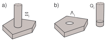
Figure 3: The union of the layer and semi-cylinder (a). The layer and the semi-cylinder (b).

The set (2.31) is obtained from the set (1.3) by going over to the stretched coordinates

$$\xi^{j}=(\eta^{j},\zeta),\ \ \ \eta^{j}=(\eta_{1}^{j},\eta_{2}^{j})=h^{-1}(y-P^{j}),\ \ \ \zeta=h^{-1}z,$$ (2.33)

see (1.2) and (1.1), and putting $h=0$ formally. Note that in the equations (2.25)-(2.30) we do not mark the variables $\xi$ and $\eta$ with the superscript $j.$ In the sequel we also omit this superscript on the functions $w$ and $\mathcal{F}$ whose restrictions on $\Lambda_{j}$ and $Q_{j}$ are denoted by $w_{0},$ $\mathcal{F}_{0}$ and $w_{j},$ $\mathcal{F}_{j},$ respectively. Moreover, let us notice that the domain $Q_{j}$ is a semi-infinite cylinder; for simplicity, we call it the semi-cylinder.

The equations (2.25), (2.26) and the boundary conditions (2.27)-(2.29) are obtained from (1.8), (1.9) and (1.10), (1.11), respectively, by the change $x\mapsto\xi.$ The transmission conditions (2.30) at the surface $\upsilon_{j}^{1}=\partial\Lambda_{j}\cup\partial Q_{j}$ result from the original conditions (1.13), (1.14) with the exponent $\alpha=0$ in (1.15). In view of a simple geometry the problem (2.25)-(2.30) can be investigated by the Fourier method (see, e.g., [48]). However, thinking about possible generalizations, see Section 5, we here realize a different approach.

The variational formulation of the problem (2.25)-(2.30) appeals to the integral identity

$$(\nabla_{\xi}w_{0},\nabla_{\xi}v_{0})_{\Lambda_{j}}+\gamma_{j}(\nabla_{\xi}w_{j},\nabla_{\xi}v_{j})_{Q_{j}}=(\mathcal{F},v)_{\Xi_{j}}\ \ \ \ \ \ \ \forall v\in\mathcal{H}_{j},$$ (2.34)

where $\nabla_{\xi}=\operatorname{grad},$ $(\ ,\ )_{\Xi}$ is the natural scalar product in the Lebesgue space $L^{2}(\Xi),$ and $\mathcal{H}_{j}$ is the completion of $C_{c}^{\infty}(\overline{\Xi_{j}})$ (infinitely differentiable functions with compact supports) in the norm

$$\|w;\mathcal{H}_{j}\|=(\|\nabla_{\xi}w;L^{2}(\Xi_{j})\|^{2}+\|w;L^{2}(\Theta_{j})\|^{2})^{1/2}$$ (2.35)

where $\Theta_{j}=\omega_{j}\times(0,1).$ Notice that a constant belongs to $\mathcal{H}_{j}$ (see, e.g., [33, 34]).

Lemma 2

An equivalent norm in $\mathcal{H}_{j}$ can be chosen as $(\|\nabla_{\xi}w;L^{2}(\Xi_{j})\|^{2}+\|\mathcal{R}^{-1}w;L^{2}(\Xi_{j})\|^{2})^{1/2}$ where $\mathcal{R}$ is a smooth positive function in $\overline{\Xi_{j}}$ such that

$$\mathcal{R}(\xi)=\zeta\text{ \ for \ }\xi\in Q_{j},\ \zeta>2,\qquad\mathcal{R}(\xi)=\rho\ln\rho\text{ \ for \ }\xi\in\Lambda_{j},\ \rho=|\eta|>2.$$ (2.36)

Proof. First of all, we observe that the cylinder $\Theta_{j}=\omega_{j}\times(0,1)$ can be obviously replaced in (2.35) by any bigger domain $\Theta_{j}^{\prime}$ with a compact closure. Next, we recall two one-dimensional Hardy inequalities

$$\int_{0}^{L}\zeta^{-2}|W(\zeta)|^{2}d\zeta \leq 4\int_{0}^{L}\left|\frac{\partial W}{\partial\zeta}(\zeta)\right|^{2}d\zeta\ \ \ \ \forall W\in C_{c}^{1}(0,L],\quad L\in(0,+\infty],$$ (2.37)

$$\int_{1}^{+\infty}\rho^{-1}|\ln\rho|^{-2}|W(\rho)|^{2}d\rho \leq 4\int_{1}^{+\infty}\rho\left|\frac{\partial W}{\partial\rho}(\rho)\right|^{2}d\rho\ \ \ \ \forall W\in C_{c}^{1}(1,+\infty).$$ (2.38)

Note that (2.38) is derived from (2.37) by the change $\rho\mapsto t=\ln\rho.$

Finally, we integrate inequality (2.37) with $W(\zeta)=(1-\chi(\zeta))w(\eta,\zeta)$ over $\omega_{j}\ni\eta$ and inequality (2.38) with $L=\infty$ and $W(\rho)=(1-\chi(\rho))w(\eta,\zeta)$ in the angular variable $\varphi\in(0,2\pi)$, where $\chi(t)=1$, if $t<1$, and $\chi(t)=0$, if $t>2$. As a result we obtain the estimates

$$\|\zeta^{-2}w;L^{2}(\omega_{j}\times(2,+\infty))\|^{2}\leq C(\|\partial_{\zeta}w;L^{2}(\omega_{j}\times(1,+\infty))\|^{2} +\|w;L^{2}(\omega_{j}\times(1,2))\|^{2}),$$ (2.39)

$$\|\rho^{-1}|\ln\rho|^{-1}w;L^{2}((\mathbb{R}^{2}\setminus\mathbb{B}_{2})\times(0,1))\|^{2} \leq C(\|\partial_{\rho}w;L^{2}((\mathbb{R}^{2}\setminus\mathbb{B}_{1})\times(0,1))\|^{2}+$$

$$+\|w;L^{2}((\mathbb{B}_{2}\setminus\mathbb{B}_{1})\times(0,1))\|^{2}).$$

where here and in the sequel $\mathbb{B}_{R}=\{\eta\in\mathbb{R}^{2}:|\eta|<R\}$ denotes the ball of radius $R$. We mention that cut-off functions were introduced in order to fulfil the conditions $W(0)=0$ in (2.37) and $W(1)=0$ in (2.38). Furthermore, we have used the relations

$$\partial_{\zeta}((1-\chi(\zeta))w(\eta,\zeta)) =(1-\chi(\zeta))\partial_{\zeta}w(\eta,\zeta)-w(\eta,\zeta)\partial_{\zeta}\chi(\zeta),$$

$$1-\chi(\zeta) =1\text{ \ for \ }\zeta>2\text{ \ and \ }\partial_{\zeta}\chi(\zeta)=0\text{ \ for \ }\zeta\notin(1,2)$$

to get the first estimate and similar relations together with the formula $d\eta=\rho d\rho d\varphi$ for the second estimate in (2.39). Choosing $\Theta_{j}^{\prime}=\{\xi\in\Xi_{j}:\rho<\max\{2,\text{diam }\omega_{j}\},\ \zeta\in(0,2)\}$ and according to (2.35), (2.36), we get $\|\mathcal{R}^{-1}w;L^{2}(\Xi_{j})\|^{2}\leq c\|w;\mathcal{H}_{j}\|^{2}$ which suffices to conclude with the proof. $\blacksquare$

By a standard argument, the Riesz representation theorem leads to the following assertion.

Proposition 3

Let the right-hand side $\mathcal{F}$ satisfy the conditions $\mathcal{RF}\in L^{2}(\Xi_{j})$ and

$$\int\nolimits_{\Xi_{j}}\mathcal{F}(\xi)d\xi=0.$$ (2.40)

Then the integral identity (2.34) (problem (2.25)-(2.30) in the differential form) has a solution $w\in\mathcal{H}_{j}$ defined up to an additive constant. Under the orthogonality condition $\int_{\Theta_{j}}w(\xi)d\xi=0$ the solution becomes unique and meets the estimate $\|w;\mathcal{H}_{j}\|^{2}\leq c\|\mathcal{RF};L^{2}(\Xi_{j})\|^{2}.$

In addition to a constant solution of the homogeneous problem (2.25)-(2.30) we shall need an unbounded solution $\mathbf{w}^{j}$ defined uniquely by its asymptotic forms

$$\mathbf{w}^{j}(\xi) =-(2\pi)^{-1}\ln\rho+o(1),\ \ \ \xi\in\Lambda_{j},\ \ \rho=|\eta|\rightarrow+\infty,$$ (2.41)

$$\mathbf{w}^{j}(\xi) =\gamma_{j}^{-1}|\omega_{j}|^{-1}\zeta+\mathbf{q}_{j}+o(1),\ \ \ \xi\in Q_{j},\ \ \zeta\rightarrow+\infty,$$ (2.42)

where $\mathbf{q}_{j}$ is a constant described below. A distinct way to find out this solution is to search for the remainder $\widehat{\mathbf{w}}^{j}\in\mathcal{H}_{j}$ in the representation

$$\mathbf{w}^{j}(\xi)=\gamma_{j}^{-1}|\omega_{j}|^{-1}X_{Q}(\zeta)-(2\pi)^{-1}X_{\Lambda}(\eta)\ln\rho+\widehat{\mathbf{w}}_{j}(\xi)$$

where $X_{Q}(\zeta)=1-\chi(\zeta)$ and $X_{\Lambda}(\eta)=1-\chi(\rho/R_{j})$ are smooth cut-off functions,

$$X_{Q}(\zeta) =0\text{ \ for \ }\zeta<1,\ \ X_{Q}(\zeta)=1\text{ \ for \ }\zeta>2,$$ (2.43)

$$X_{\Lambda}(\eta) =0\text{ \ for \ }|\eta|<R_{j},\ \ X_{\Lambda}(\eta)=1\text{ \ for \ }|\eta|>2R_{j},$$

and radius $R_{j}>0$ is fixed such that $\overline{\omega_{j}}\subset\{\eta:|\eta|<R_{j}\}.$ The remainder must satisfy problem (2.25)-(2.30)  with the smooth and compactly supported right-hand sides $\mathcal{F}_{0}^{j}=-(2\pi)^{-1}[\Delta_{\xi},X_{\Lambda}]\ln\rho,\ \mathcal{F}_{j}^{j}=|\omega_{j}|^{-1}[\Delta_{\xi},X_{Q}]\zeta,$ where $[\Delta_{\xi},X]$ is the commutator of the Laplace operator and a cut-off function $X,$

$$[\Delta_{\xi},X]w=2\nabla_{\xi}w\cdot\nabla_{\xi}X+w\Delta_{\xi}X.$$ (2.44)

Clearly, $\mathcal{RF}\in L^{2}(\Xi_{j})$ and, to get $\widehat{\mathbf{w}}_{j},$ we only need to verify the validity of the orthogonality condition (2.40) in Proposition 3. It is assured by the following calculation:

$$\frac{1}{2\pi}\int_{\Lambda_{j}}[\Delta_{\xi},X_{\Lambda}]\ln\frac{1}{\rho}d\xi+\frac{1}{|\omega_{j}|}\int_{Q_{j}}[\Delta_{\xi},X_{Q}]\zeta d\xi$$ (2.45)

$$=\frac{1}{2\pi}\lim_{T\rightarrow+\infty}\int_{0}^{1}\int_{\mathbb{B}_{T}\setminus\mathbb{B}_{R_{j}}}\Delta_{\xi}\left(X_{\Lambda}(\eta)\ln\frac{1}{\rho}\right)d\eta d\zeta+\frac{1}{|\omega_{j}|}\lim_{T\rightarrow+\infty}\int_{\omega_{j}}\int_{1}^{T}\Delta_{\xi}(X_{Q}(\zeta)\zeta)d\zeta d\eta$$

$$=\frac{1}{2\pi}\lim_{T\rightarrow+\infty}\int_{\partial\mathbb{B}_{T}}\left.\frac{\partial}{\partial\rho}\ln\frac{1}{\rho}\right|_{\rho=T}~{}ds_{\eta}+\frac{1}{|\omega_{j}|}\lim_{T\rightarrow+\infty}\int_{\omega_{j}}\left.\frac{\partial\zeta}{\partial\zeta}\right|_{\zeta=T}~{}d\eta=-1+1=0.$$

The decompositions (2.41) and (2.42) are supported by the Fourier method where $\mathbf{q}_{j}$ is a constant which is defined uniquely and depends on $\gamma_{j}$ and $\omega_{j}$ (cf. Remark 5).

We finally formulate a representation of a solution to the homogeneous problem (2.25)-(2.30) which, for example, follows from our consideration of the decoupled problems in the next section.

Theorem 4

Any solution $w\in H_{loc}^{1}(\Xi_{j})$ of the homogeneous problem (2.25)-(2.30) satisfying the estimates

$$|w_{0}(\xi)|\leq c\ln(1+\rho)\text{\ in }\Lambda_{j},\ \rho>R_{j},\quad|w_{j}(\xi)|\leq c\,\zeta\text{ \ in }Q_{j},\ \zeta\geq 2,$$ (2.46)

is a linear combination $c_{0}+c_{1}\mathbf{w}^{j}$ with some coefficients $c_{i}$ and the constructed special solution $\mathbf{w}^{j}$.

2.4 The limit problems in a perforated layer and in a semi-cylinder

In the case $\alpha=1,$ equation (1.14) contains the big factor $h^{-1}$ and, therefore, after the coordinate dilation $x\mapsto\xi^{j},$ see (2.33), the transmission conditions (1.13), (1.14) decouple while junction (2.31) splits into the perforated layer and the semi-cylinder (2.32), see fig. 3,b. We shall see in Section 3.1 that the transmission conditions give rise to the Dirichlet condition on the hole surface $\upsilon_{j}^{1}\subset\partial\Lambda_{j}$ and to the Neumann condition on the ring $\upsilon_{j}^{1}\subset\partial Q_{j}$ near the cylinder end. In this way, to describe the boundary layer phenomenon, we have to deal with two problems, namely the mixed boundary value problem

$$-\Delta_{\xi}W_{0}(\xi) =0,\ \xi\in\Lambda_{j},\ \ \partial_{\zeta}W_{0}(\eta,0)=\partial_{\zeta}W_{0}(\eta,1)=0,\ \ \ \eta\in\mathbb{R}^{2}\setminus\overline{\omega_{j}},$$ (2.47)

$$W_{0}(\xi) =g_{0}(\xi),\ \ \xi\in\upsilon_{j}^{1},$$

in the perforated layer and the Neumann problem in the semi-cylinder

$$-\gamma_{j}\Delta_{\xi}W_{0}(\xi) =0,\ \xi\in Q_{j},\ \ \gamma_{j}\partial_{\nu}W_{0}(\eta,\zeta)=g_{j}(\eta,\zeta),\ \ \ (\eta,\zeta)\in\partial\omega_{j}\times\mathbb{R}_{+},$$ (2.48)

$$\gamma_{j}\partial_{\zeta}W_{0}(\eta,0) =0,\ \ \eta\in\omega_{j}.$$ (2.49)

Both the problems permit separation of variables and are rather standard in the asymptotic analysis of rods and perforated plates, even isolated (cf., respectively, the monographs [30, 20, 45, 31] and the papers [33, 7]). We here present only some comprehensible pieces of information on them which will be used for asymptotic structures in Section 3.

First of all, a solution of the homogeneous problem (2.47) with the logarithmical growth at infinity, cf. (2.46), does not depend on the variable $\zeta$ and takes the form of the logarithmic potential $\mathbf{W}_{j}(\eta)$ that is a harmonic function in $\mathbb{R}^{2}\setminus\overline{\omega_{j}}$ which vanishes at $\partial\omega_{j}$ and admits the representation

$$\mathbf{W}_{j}(\eta)=(2\pi)^{-1}(-\ln\rho+\ln c_{\log}(\omega_{j}))+O(\rho^{-1}),\ \ \rho\rightarrow+\infty,$$ (2.50)

where $c_{\log}(\omega_{j})$ is the logarithmic capacity of the set $\overline{\omega_{j}}$ (see, e.g., [46, 25]).

Remark 5

Owing to (2.42) and (2.41), the difference $\mathbf{w}^{j}(\xi)-\mathbf{q}^{j}$ also can be represented in form (2.50) inside the layer $\Lambda_{j}$ as $-(2\pi)^{-1}\ln\rho-\mathbf{q}^{j}+O(\rho^{-1}),\rho\rightarrow+\infty,$ so that the quantity $e^{-2\pi\mathbf{q}^{j}}$ could be called the logarithmic capacity in the junction of the layer and semi-cylinder (2.31).

Lemma 6

There holds the equality ${\displaystyle\int_{\partial\omega_{j}}}\partial_{\nu}\mathbf{W}_{j}(\eta)ds_{\eta}=1.$

Proof. We just repeat the calculation (2.45):

$$\int_{\partial\omega_{j}}\partial_{\nu}\mathbf{W}_{j}(\eta)ds_{\eta}=-\lim_{T\rightarrow+\infty}\int_{\partial\mathbb{B}_{T}}\frac{\partial\mathbf{W}_{j}}{\partial\rho}(\eta)ds_{\eta}=-\frac{1}{2\pi}\lim_{T\rightarrow+\infty}\int_{\partial\mathbb{B}_{T}}\frac{\partial}{\partial\rho}\ln\frac{1}{\rho}ds_{\eta}=1.\ \ \ \ \blacksquare$$

As for the Neumann problem in the semi-cylinder $Q_{j},$ we will use the following assertion which is based on the Fourier method.

Lemma 7

Let the right-hand side $g_{j}\in L^{2}(\partial\omega_{j}\times\mathbb{R}_{+})$ in problem (2.48), (2.49) possess a compact support. Then the problem has a solution $W_{j}$ which is defined up to an additive constant and gets the form

$$W_{j}(\eta,\zeta)=C_{j}\zeta+C_{0j}+O(e^{-\delta\zeta}),\ \ \zeta\rightarrow+\infty,$$ (2.51)

where $C_{0j}$ is a constant, $\delta$ is some positive number and

$$C_{j}=-\frac{1}{\gamma_{j}|\omega_{j}|}\int_{0}^{+\infty}\int_{\partial\omega_{j}}g_{j}(\eta,\zeta)ds_{\eta}d\zeta.$$

Remark 8

To describe the boundary layer effect at the rod ”soles” $\omega_{j}^{h}(l_{j})$ with the Dirichlet conditions (1.12), one has to consider the mixed boundary value problem in the semi-cylinder $Q_{j},$ too, which now is obtained as a result of the coordinate dilation $x\mapsto(h^{-1}(y-P^{j}),h^{-1}(l_{j}-z)),$ cf. (2.33). This problem consists of equations (2.48) and the Dirichlet condition at the cylinder end

$$W_{j}(\eta,0)=g_{j}^{l}(\eta),\ \ \eta\in\omega_{j}.$$ (2.52)

Although we do not involve solutions of (2.48), (2.52) into asymptotic structures in Section 3, we again mention the monographs [30, 20, 45, 31] where this problem was investigated and applied. $\blacksquare$

3 Constructing asymptotic expansions

Both cases $\alpha=1$ and $\alpha=0$ are investigated by means of the method of matched asymptotic expansions, see, e.g, the monographs [50, 17] and [30, Ch.2], so that the asymptotic procedures for the contrasting and homogeneous junctions defined according to (1.15), (1.16) look quite similar although provide very different formulas for the main asymptotic terms in the solution $u(h,x)$ of problem (1.8)-(1.14). An evident distinction of final formulas originates in the different structure of the inner expansions composed from solution to the limit problems (2.47)-(2.49) and (2.25)-(2.30) posed on infinite domains depicted in fig. 3, a and b, respectively. In other words, the asymptotic structure of solutions in the junction (1.3) is crucially prescribed by boundary layer effects around the junction zones.

3.1 The case $\alpha=1.$

Based on our preliminary consideration in Section 2, we assume the asymptotic ansätze (2.3) in the rods $\Omega_{j}(h)$ and (2.9) in the plate $\Omega_{\bullet}(h).$ The main term $U_{j}^{0}$ in (2.3) satisfies the ordinary differential equation (2.5) and the Dirichlet condition (2.6), however a condition at $z=0$ is still absent and needs to be derived. The main term $U_{0}^{0}$ in (2.9) is a singular solution of the Neumann problem (2.19), (2.12) in the punctured domain (2.18) while coefficients in its representation (2.20) also remain unknown. In order to find out appropriate values of the coefficients $A_{0},A_{1},...,A_{J}$ as well as right-hand sides in

$$-\gamma_{j}|\omega_{j}|\partial_{z}U_{j}^{0}(0)=G_{j}^{0}$$ (3.1)

we construct inner asymptotic expansions in the vicinity of the points $P^{1},...,P^{J}.$ Namely, in a neighborhood $V_{j}$ of $P^{j}$ where the stretched coordinates (2.33) were defined, we search for the asymptotic forms

$$u(h,x) =W_{j}^{0}(\eta^{j},\zeta)+hW_{j}^{1}(\eta^{j},\zeta)+...\ \ \ \text{ in }\Omega_{j}(h)\cap V_{j},$$ (3.2)

$$u(h,x) =W_{0j}^{0}(\eta^{j},\zeta)+...\text{ \ \ \ \ in }\Omega_{0}(h)\cap V_{j}.$$ (3.3)

Aiming to determine the entries $W_{j}^{0}$ and $W_{j}^{1}$ in (3.2), we apply the Taylor formula to $U_{j}^{0}$ and write

$$U_{j}^{0}(z)=U_{j}^{0}(0)+z\partial_{z}U_{j}^{0}(0)+O(z^{2})=U_{j}^{0}(0)+h\zeta\partial_{z}U_{j}^{0}(0)+O(h^{2}\zeta^{2}).$$ (3.4)

The matching procedure (see, e.g., [50, 17], [30, Ch.2]) requires the entries to inherit an asymptotic behavior from terms in (3.4). In this way we readily set

$$W_{j}^{0}(\eta^{j},\zeta)=U_{j}^{0}(0)$$ (3.5)

and, furthermore, we fix the behavior of $W_{j}^{1}$ at infinity as follows:

$$W_{j}^{1}(\eta^{j},\zeta)=\zeta\partial_{z}U_{j}^{0}(0)+o(1),\ \ \zeta\rightarrow+\infty.$$ (3.6)

The constant function (3.5) does not bring a discrepancy into the transmission conditions (1.14). Satisfying the other transmission condition (1.13), we subject $W_{0j}^{0}$ to the Dirichlet condition

$$W_{0j}^{0}(\eta^{j},\zeta)=U_{j}^{0}(0),\ \ \ \ (\eta^{j},\zeta)\in\upsilon_{j}^{1}=\partial\omega_{j}\times(0,1).$$

on the lateral boundary of the perforated layer $\Lambda_{j}$, see (2.32) and (1.7). As in Section 2.4, the harmonic function $W_{0j}^{0}$ satisfies the homogeneous Neumann condition at the bases of the layer and, hence, it becomes independent of the variable $\zeta$. With some coefficient $A_{j}$, we thus set

$$W_{0j}^{0}(\eta^{j},\zeta)=U_{j}^{0}(0)+A_{j}\mathbf{W}_{j}(\eta^{j}).$$ (3.7)

In view of (3.2), (3.3), and (3.5), (3.7), the transmission condition (1.14) converts into

$$h^{-1}\gamma_{j}\partial_{\nu}(U_{j}^{0}(0)+hW_{j}^{1}(\xi^{j}))=\partial_{\nu}(U_{j}^{0}(0)+A_{j}\mathbf{W}_{j}(\eta^{j})),\ \ \ \xi^{j}\in\upsilon_{j}^{1},$$

and, hence, yields the following Neumann condition on the ring $\upsilon_{j}^{1}\subset\partial Q_{j}$ near the cylinder end:

$$\gamma_{j}\partial_{\nu}W_{j}^{1}(\eta^{j},\zeta)=A_{j}\partial_{\nu}\mathbf{W}_{j}(\eta^{j}),\ \ \ (\eta^{j},\zeta)\in\upsilon_{j}^{1}.$$

In other words, the term $W_{j}^{1}$ in (3.2) satisfies problem (2.48), (2.49) with the right-hand side

$$g_{j}(\eta,\zeta)=A_{j}\partial_{\nu}\mathbf{W}_{j}(\eta^{j}),\ \zeta\in(0,1),\quad g_{j}(\eta,\zeta)=0,\ \zeta>1.$$

Lemmas 7 and 6 ensure the existence of the unique solution $W_{j}^{1}$ of the asymptotic form (2.51) where

$$C_{0j}=0,\ \ C_{j}=\frac{A_{j}}{\gamma_{j}|\omega_{j}|}\int_{0}^{1}\int_{\partial\omega_{j}}\partial_{\nu}\mathbf{W}_{j}(\eta^{j})ds_{\eta}d\zeta=-\frac{A_{j}}{\gamma_{j}|\omega_{j}|}.$$

Comparing this form with (3.6), we conclude that condition (3.1) provides

$$G_{j}^{0}=A_{j}.$$ (3.8)

The limit problem (2.5), (2.6), (3.1) has the unique solution

$$U_{j}^{0}(z)=U_{j}^{\#}(z)+A_{j}\gamma_{j}^{-1}|\omega_{j}|^{-1}(l_{j}-z_{j})$$ (3.9)

where $U_{j}^{\#}$ is independent of $A_{j}$ and verifies

$$-\gamma_{j}|\omega_{j}|\partial_{z}^{2}U_{j}^{\#}(z) =|\omega_{j}|f_{j}^{0}(z),\ \ z\in(0,l_{j}),\ \ U_{j}^{\#}(l_{j})=0,$$ (3.10)

$$-\gamma_{j}|\omega_{j}|\partial_{z}U_{j}^{\#}(0) =0.$$ (3.11)

We obviously have

$$U_{j}^{\#}(0)=\frac{1}{\gamma_{j}}\int_{0}^{l_{j}}(l_{j}-z)f_{j}^{0}(z)dz.$$ (3.12)

Using decomposition (2.50) in (3.7) yields

$$W_{0j}^{0}(\eta^{j},\zeta) =U_{j}^{0}(z)-(2\pi)^{-1}A_{j}(\ln\rho_{j}-\ln c_{\log}(\omega_{j}))+O(\rho_{j}^{-1})=$$ (3.13)

$$=U_{j}^{0}(0)-(2\pi)^{-1}A_{j}(\ln r_{j}-\ln h-\ln c_{\log}(\omega_{j}))+O(hr_{j}^{-1}).$$

On the other hand, by (2.15), the linear combination (2.20) decomposes as follows:

$$U_{0}^{0}(y)=U_{\bot}^{0}(P^{j})+A_{0}+(2\pi)^{-1}A_{j}\ln r_{j}^{-1}+{\textstyle\sum\nolimits_{k}}A_{k}G_{kj}+O(r_{j}).$$ (3.14)

Note that $\ln r_{j}$ in (3.13) got the same factor $-(2\pi)^{-1}A_{j}$ as in (3.14) due to our choice (3.7).

The matching procedure requires that the sums of the terms detached in (3.13) and (3.14) coincide with each other. Thus, in view of (3.9), we obtain the relations

$$U_{j}^{\#}(0)+\gamma_{j}^{-1}|\omega_{j}|^{-1}A_{j}+(2\pi)^{-1}A_{j}(\ln h+\ln c_{\log}(\omega_{j}))=U_{\bot}^{0}(P^{j})+A_{0}+{\textstyle\sum\nolimits_{k}}A_{k}G_{kj}$$ (3.15)

with $j=1,...,J$. In order to write them differently

$$M(\ln h)\overrightarrow{A}=-A_{0}E+\overrightarrow{F}$$ (3.16)

we introduce the columns

$$\overrightarrow{A} =(A_{1},...,A_{J})^{\top}\in\mathbb{R}^{J}$$ (3.17)

$$E =(1,...,1)^{\top}\in\mathbb{R}^{J},\ \ \ \overrightarrow{F}=\overrightarrow{U}^{\#}(0)-\overrightarrow{U}_{\bot}^{0}(P),$$ (3.18)

$$\overrightarrow{U}^{\#}(0) =(U_{1}^{\#}(0),...,U_{J}^{\#}(0))^{\top},\ \ \ \overrightarrow{U}_{\bot}^{0}(P)=(U_{\bot}^{0}(P^{1}),...,U_{\bot}^{0}(P^{J}))^{\top},$$

while $\top$ stands for transposition, and the matrix of size $J\times J$

$$M(\ln h)=-(2\pi)^{-1}\ln h~{}\mathbb{I}+G-L$$ (3.19)

where $\mathbb{I}$ is the unit $J\times J$-matrix, $G$ is defined in (2.16) and $L$ is a diagonal matrix, namely,

$$L=diag\{(2\pi)^{-1}\ln c_{\log}(\omega_{1})+\gamma_{1}^{-1}|\omega_{1}|^{-1},...,(2\pi)^{-1}\ln c_{\log}(\omega_{J})+\gamma_{J}|\omega_{J}|^{-1}\}.$$

Matrix (3.19) is symmetric, see (2.17), and positive definite for $h\in(0,h_{0}]$ when $h_{0}\in(0,1)$ is sufficiently small and, therefore, $-\ln h=|\ln h|$. We then have

$$\overrightarrow{A}=-A_{0}M(\ln h)^{-1}E+M(\ln h)^{-1}\overrightarrow{F}.$$ (3.20)

Recalling restriction (2.21) in Proposition 1, we multiply (3.20) scalarly by the column $E$ and obtain

$$A_{0}=m(\ln h)^{-1}(\langle f_{0}^{0}\rangle_{0}+E^{\top}M(\ln h)^{-1}\overrightarrow{F})$$ (3.21)

with the positive coefficient

$$m(\ln h)=E^{\top}M(\ln h)^{-1}E=O(|\ln h|^{-1}).$$ (3.22)

Inserting (3.21) into (3.20) finishes our construction of the terms $U_{0}^{0}$ in (2.20) and $U_{j}^{0}$ in (3.9) of the asymptotic ansätze (2.3), (2.9). Due to (3.19) and (3.22) all their ingredients with exception of $U_{\bot}^{0}$ and $U_{j}^{\#}$ are rational functions in $\ln h$ while the estimates

$$|A_{0}(\ln h)|\leq c|\ln h||\overrightarrow{F}|,\ \ \ |A_{j}(\ln h)|\leq c|\overrightarrow{F}|,\ \ \ j=1,...,J,$$ (3.23)

are valid where, according to the compact embeddings $H^{2}(\omega_{0})\subset C(\omega_{0})$ and $H^{1}(0,l_{j})\subset C[0,l_{j}],$

$$|\overrightarrow{F}|\leq|\overrightarrow{U}_{\bot}^{0}(P)|+|\overrightarrow{U}^{\#}(0)|\leq c(\|U_{\bot}^{0};H^{2}(\omega_{0})\|+{\textstyle\sum\nolimits_{j}}\|U_{j}^{\#};H^{1}(0,l_{j})\|).$$ (3.24)

The inner expansions (3.2) and (3.3) are completed, too.

3.2 The particular case $J=1$ and $\alpha=1$.

The mushroom shape of the junction, fig. 2,b, simplifies all the above-obtained asymptotic terms because matrix (3.19) at $J=1$ becomes the scalar

$$M(\ln h)=(2\pi)^{-1}(|\ln h|-\ln c_{\log}(\omega_{1}))+G_{11}-\gamma_{1}^{-1}|\omega_{1}|^{-1}$$

and, moreover, $E=1\in\mathbb{R}$ and $m(\ln h)=M(\ln h)^{-1}$ in (3.22). In view of (2.24) and (3.12), now formulas (3.21) and (3.20) read as follows:

$$A_{0}(\ln h)=M(\ln h)\langle f_{0}^{0}\rangle_{0}+\frac{1}{\gamma_{1}}\int_{0}^{l_{1}}(l_{1}-z)f_{1}^{0}(z)dz-\int_{\omega_{0}}G_{1}(y)f_{0}^{0}(y)dy,\quad A_{1}(\ln h)=-\langle f_{0}^{0}\rangle_{0}.$$

The latter apparently coincides with (2.21). Only under the orthogonality condition $\langle f_{0}^{0}\rangle_{0}=0$ the term $A_{0}(\ln h)$ in (2.20) and the solution $U_{0}^{0}$ itself stay bounded as $h\rightarrow+0$ while $A_{1}(\ln h)G_{1}(y)$ disappears, too.

Let us outline the asymptotic structures of the solution $u(h,x)$ to problem (1.8), (1.9), (1.19), (1.11)-(1.14) with the Dirichlet condition on the lateral side of the plate $\Omega_{0}$. For any $J$, the outer (2.3), (2.9) and inner (3.2), (3.3) expansions, of course, keep their forms but now the constant term $A_{0}$ in the singular solution

$$U_{0}^{0}(y)=U_{0}^{\#}(y)+{\textstyle\sum\nolimits_{j}}A_{j}G_{j}(y)$$ (3.25)

is absent while $U_{0}^{\#}\in H^{2}(\omega_{0})$ is nothing but the unique solution of

$$-\Delta_{y}U_{0}^{\#}(y)=f_{0}^{0}(y),\ y\in\omega_{0},\ \ \ \ \ \ \ \ U_{0}^{\#}(y)=0,\ y\in\partial\omega_{0},$$ (3.26)

and $G_{j}(y)=G(y,P^{j})$ denotes the standard Green function of the Dirichlet Laplacian. Although the matching procedure resulting in the system (3.16) with $A_{0}=0$ remains the same as in Section 3.1, properties of the coefficient column (3.17) in (3.25) change crucially. Examining the solution

$$\overrightarrow{A} =(A_{1},...,A_{J})^{\top}=M(\ln h)^{-1}(\overrightarrow{U}^{\#}(0)-\overrightarrow{U}_{0}^{\#}(P)),$$ (3.27)

$$\overrightarrow{U}_{0}^{\#}(P) =(U_{0}^{\#}(P^{1}),...,U_{0}^{\#}(P^{J}))^{\top}$$

of the algebraic system, one sees that, instead of (3.23), there hold the estimates $|A_{j}(\ln h)|\leq c|\ln h|^{-1}$. In other words, singular components in (3.25) get small coefficients.

3.3 The case $\alpha=0.$

As mentioned in Section 1.2, a change of the exponent $\alpha$ in relation (1.15), comparing properties of elements of junction (1.3), may crucially modify the asymptotic ansätze for the solution $u(h,x)$ of problem (1.8)-(1.14). At $\alpha=0,$ for example in the homogeneous ($\gamma_{j}=1$) junction, we replace expansions (2.9) and (2.3), suitable for $\alpha=1,$ with the following ones involving terms of order $h^{-1}:$

$$u_{0}(h,x) =h^{-1}a_{0}+U_{0}^{0}(y)+hU_{0}^{1}(y,\zeta)+h^{2}U_{0}^{2}(y,\zeta)+...,$$ (3.28)

$$u_{j}(h,x) =h^{-1}U_{j}^{-1}(z)+U_{j}^{0}(z)+hU_{j}^{1}(\eta^{j},z)+h^{2}U_{j}^{2}(\eta^{j},z)+...,$$ (3.29)

where $a_{0}$ is a constant to be computed and, as we will confirm below, $U_{j}^{-1}$ are linear functions,

$$U_{j}^{-1}(z)=a_{0}(1-l_{j}^{-1}z).$$ (3.30)

Since a constant and the linear function (3.30) verify the homogeneous differential equations (1.8) and (1.9) as well as the boundary conditions (1.10) and (1.11), (1.12), the terms $U_{0}^{k}$ in (3.28) and $U_{j}^{k}$ in (3.29) with $k\geq 0$ keep their forms given in Sections 2.2 and 2.1, respectively. Furthermore, the main asymptotic terms in the above ansätze satisfy the transmission condition (1.13) but leave a discrepancy $O(1)$ in the condition (1.14). Hence, the inner expansion which substitutes for (3.2) and (3.3), looks as follows:

$$u(h,x)=h^{-1}w_{j}^{-1}(\eta^{j},\zeta)+w_{j}^{0}(\eta^{j},\zeta)+...\ \ \ \text{in \ }\Xi(h)\cap V_{j}$$ (3.31)

where $w_{j}^{-1}$ and $w_{j}^{0}$ are to be chosen as appropriate solutions of the homogeneous problem (2.25)-(2.30) studied in Section 2.3. Evidently, due to (3.28)-(3.30) we set

$$w_{j}^{-1}(\eta^{j},\zeta)=a_{0}.$$ (3.32)

Moreover, the matching procedure and formula (3.30) requires that

$$w_{j}^{0}(\eta^{j},\zeta)=-a_{0}l_{j}^{-1}\zeta+O(1)\text{ \ \ in }Q_{j},\ \ \ \zeta\rightarrow+\infty.$$ (3.33)

All solutions of the homogeneous problem (2.25)-(2.30) with the asymptotic behavior (3.33) have been described in Theorem 4 and, therefore,

$$w_{j}^{0}(\eta^{j},\zeta)=-a_{0}l_{j}^{-1}|\omega_{j}|\gamma_{j}\mathbf{w}^{j}(\eta^{j},\zeta)+b_{j}$$ (3.34)

with a certain constant $b_{j}.$ Using decomposition (2.41) of $\mathbf{w}^{j}$ in the layer $\Lambda_{j},$ we now obtain that

$$h^{-1}w_{j}^{-1}(\eta^{j},\zeta)+w_{j}^{0}(\eta^{j},\zeta) =h^{-1}a_{0}+a_{0}\gamma_{j}|\omega_{j}|(2\pi l_{j})^{-1}\ln\rho_{j}+b_{j}+O(\rho_{j}^{-1})=$$ (3.35)

$$=h^{-1}a_{0}+a_{0}\gamma_{j}|\omega_{j}|(2\pi l_{j})^{-1}(\ln r_{j}-\ln h)+b_{j}+O(hr_{j}^{-1})\ \ \ \ \text{in }\Lambda_{j}.$$

Matching (3.35) and (3.28) subjects the function $U_{0}^{0}$ to the conditions

$$U_{0}^{0}(y)=a_{0}\gamma_{j}|\omega_{j}|(2\pi l_{j})^{-1}(\ln r_{j}-\ln h)+b_{j}+O(r_{j}),\ \ r_{j}\rightarrow 0.$$ (3.36)

In other words, representation (2.20) of the singular solution $U_{0}^{0}$ to the limit problem (2.19), (2.12) involves the coefficients

$$A_{j}=-a_{0}l_{j}^{-1}|\omega_{j}|\gamma_{j}.$$ (3.37)

Furthermore, restriction (2.21) requires that

$$a_{0}=(l_{1}^{-1}|\omega_{1}|\gamma_{1}+...+l_{J}^{-1}|\omega_{J}|\gamma_{J})^{-1}\langle f_{0}^{0}\rangle_{0}.$$ (3.38)

Thus, the main asymptotic terms in expansions (3.28) and (3.29) have been determined.

The second term $U_{0}^{0}$ of the outer expansion (3.28) in the perforated plate $\Omega_{\bullet}(h)$ is defined up to the constant addendum $A_{0}$ in (2.20). Comparing formulas (2.20), (2.15) and (3.36) yields

$$b_{j}=U_{\bot}^{0}(P^{j})+A_{0}+{\textstyle\sum\nolimits_{k}}A_{k}G_{kj}(y)+a_{0}\gamma_{j}|\omega_{j}|(2\pi l_{j})^{-1}\ln h.$$ (3.39)

Since, by (3.32), (3.34) and (2.42), we have

$$h^{-1}w_{j}^{-1}(\eta^{j},\zeta)+w_{j}^{0}(\eta^{j},\zeta) =h^{-1}a_{0}-a_{0}l_{j}^{-1}\zeta+a_{0}|\omega_{j}|\gamma_{j}\mathbf{q}_{j}+b_{j}+O(e^{-\delta\zeta})=$$

$$=h^{-1}a_{0}(1-l_{j}^{-1}z)+b_{j}+a_{0}|\omega_{j}|\gamma_{j}\mathbf{q}_{j}+O(e^{-\delta z/h})\text{ \ \ in }Q_{j},$$

matching the inner expansion (3.31) with the outer expansion (3.29) specified as

$$h^{-1}U_{j}^{-1}(z)+U_{j}^{0}(z)=h^{-1}a_{0}(1-l_{j}^{-1}z)+U_{j}^{0}(0)+O(z)$$

leads to the boundary condition

$$U_{j}^{0}(0)=b_{j}+a_{0}\gamma_{j}|\omega_{j}|\mathbf{q}_{j}.$$ (3.40)

According to (3.39), the solution of the limit problem (2.5), (2.6) and (3.40) in $(0,l_{j})$ looks as follows:

$$U_{j}^{0}(z;\ln h)=(A_{0}+a_{0}\gamma_{j}|\omega_{j}|(2\pi l_{j})^{-1}\ln h)(1-l_{j}^{-1}z)+U_{j}^{\#}(z)$$ (3.41)

where $A_{0}$ is not fixed yet but $U_{j}^{\#}$ does not depend on $\ln h$ and is unambiguously defined as a unique solution of problem (3.10) equipped with the Dirichlet condition

$$U_{j}^{\#}(0)=U_{\bot}^{0}(P^{j})+{\textstyle\sum\nolimits_{k}}A_{k}G_{kj}(y)+a_{0}\gamma_{j}|\omega_{j}|\mathbf{q}_{j}$$

instead of the Neumann ones (3.11). One may detect $A_{0}$ by constructing next asymptotic terms but we avoid to encumber our paper with computations of access, although we will get troubles with the unknown $A_{0}$ in the justification procedure. We only mention that $A_{0}=A_{0}(\ln h)$ could be proved to depend linearly on $\ln h.$ In this way terms (3.41) of the asymptotic ansätze (3.29) on the rods become linear in $\ln h,$ too. Recall that $a_{0}$ and the constructed terms $U_{j}^{-1}$, $U_{0}^{0}-A_{0}$ are independent of $\ln h.$

3.4 The particular case $J=1$ and $\alpha=0.$

For the junction $\Xi(h)=\Omega_{0}(h)\cup\Omega_{1}(h)$ of a plate and a single rod, the main asymptotic terms in ansätze (3.28) and (3.29) are determined by the formulas $a_{0}=\gamma_{1}^{-1}|\omega_{j}|^{-1}l_{1}\langle f^{0}_{0}\rangle_{0}$ and (3.30). Other formulas in the previous section only need the specification $j=1$.

As in the case $\alpha=1,$ a simplification of asymptotic ansätze occurs in problem (1.8), (1.9), (1.19), (1.11)-(1.14) with the Dirichlet condition on the lateral side of the plate $\Omega_{0}(h).$ First of all, terms of order $h^{-1}$ disappear and we return to the outer expansions (2.3) and (2.9). Moreover, the main term $U_{0}^{0}$ in (2.9) is no longer singular and implies a solution in $H^{2}(\omega_{0})$ of the Dirichlet problem (3.26). Thus, the values $U_{0}^{0}(P^{j})$ are defined properly and the main terms $U_{j}^{0}$ in (2.3) become nothing but solutions of the Dirichlet problems in the interval $(0,l_{j})$ composed from (2.5), (2.6) and

$$U_{j}^{0}(0)=U_{0}^{0}(P^{j}).$$ (3.42)

Owing to such elementary asymptotic structures it is not even necessary to deal with inner expansions in the justification scheme. However, we mention that the inner expansion (3.31), of course, loses the term $h^{-1}w_{j}^{-1}$ and gains the constant term $w_{j}^{0}(\xi^{j})=U^{0}(P^{j}).$

4 Estimation of the asymptotic remainders

Since, in view of our consideration in Section 3, boundary layer effects play an important role in the obtained asymptotic structures, error estimates for the asymptotic expansions are seriously based on certain weighted inequalities presented below. A general approach for derivation of such inequalities on thin domains and junctions with different limit dimensions can be found in the review paper [42].

4.1 Weighted estimates on thin elements of the junction

We integrate in $y\in\omega_{j}^{h}$ the Hardy inequality (2.37) with $L=l_{j},\zeta=l_{j}-z,W(\zeta)=u_{j}(y,l_{j}-\zeta)$, which is true due to the condition $u_{j}(y,l_{j})=0,$ cf. (1.12), and we obtain

$$\||l_{j}-z|^{-1}u_{j};L^{2}(\Omega_{j}(h))\|\leq 2\|\partial_{z}u_{j};L^{2}(\Omega_{j}(h))\|.$$ (4.1)

Furthermore, setting

$$\overline{u}_{j}(z)=\frac{1}{\operatorname*{mes}_{2}\omega_{j}^{h}}\int_{\omega_{j}^{h}}u_{j}(y,z)dy,$$ (4.2)

the Poincaré inequality on cross-sections of the rod $\Omega_{j}(h)$ yields

$$\|u_{j}-\overline{u}_{j};L^{2}(\Omega_{j}(h))\|\leq c(\omega_{j})h\|\nabla_{y}u_{j};L^{2}(\Omega_{j}(h))\|$$ (4.3)

where $c(\omega_{j})^{-2}$ is the first positive eigenvalue of the Neumann Laplacian in the domain $\omega_{j}.$

For $u_{0}\in H^{1}(\Omega_{0}(h)),$ we set

$$\overline{u}_{0}(y)=\frac{1}{h}\int_{0}^{h}u_{0}(y,z)dz,\ \ \ u_{0}(x)=u_{\bot}(x)+b_{0},\quad b_{0}=\frac{1}{\operatorname*{mes}_{3}\Omega_{0}(h)}\int_{\Omega_{0}(h)}u_{0}(x)dx.$$ (4.4)

Similarly to (4.3), we have

$$\|u_{0}-\overline{u}_{0};L^{2}(\Omega_{0}(h))\|\leq\pi^{-1}h\|\partial_{z}u_{0};L^{2}(\Omega_{0}(h))\|$$ (4.5)

Using the change of variables $x\mapsto(y,\zeta)=(y,h^{-1}z)$ and therefore transforming $\Omega_{0}(h)$ into the domain $\Omega_{0}(1)=\omega_{0}\times(0,1)$ independent of $h$, we obtain

$$\|u_{\bot};L^{2}(\Omega_{0}(h))\|^{2} =\|u_{0}-b_{0};L^{2}(\Omega_{0}(h))\|^{2}=h\|u_{0}-b_{0};L^{2}(\Omega_{0}(1))\|^{2}\leq$$ (4.6)

$$\leq c_{0}h\|\nabla_{(y,\zeta)}u_{0};L^{2}(\Omega_{0}(1))\|^{2}\leq$$

$$\leq c_{0}h(\|\nabla_{y}u_{0};L^{2}(\Omega_{0}(1))\|^{2}+\|\partial_{\zeta}u_{0};L^{2}(\Omega_{0}(1))\|^{2})\leq$$

$$\leq c_{0}h(\|\nabla_{y}u_{0};L^{2}(\Omega_{0}(1))\|^{2}+h^{-2}h_{0}^{2}\|\partial_{\zeta}u_{0};L^{2}(\Omega_{0}(1))\|^{2})=$$

$$=c_{0}(\|\nabla_{y}u_{0};L^{2}(\Omega_{0}(h))\|^{2}+h_{0}^{2}\|\partial_{z}u_{0};L^{2}(\Omega_{0}(h))\|^{2})\leq$$

$$\leq c_{0}\max\{1,h_{0}^{2}\}\|\nabla_{x}u_{0};L^{2}(\Omega_{0}(h))\|^{2},$$

where $c_{0}$ is the first positive eigenvalue of the Neumann Laplacian in $\Omega_{0}(1).$ Note that in (4.6) we have used the Poincaré inequality in $\Omega_{0}(1)$ based on the orthogonality condition $(u_{0}-b_{0},1)_{\Omega_{0}(1)}=0$ in (4.4).

4.2 Weighted estimates on the whole junction

In relation (4.1) we give an inequality for the restriction $u_{j}=u|_{\Omega_{j}(h)}$. However, the relations (4.5) and (4.6) do not provide an inequality for the restriction $u_{0}=u|_{\Omega_{0}(h)}$ but only for its components $u_{0}-\overline{u}_{0}$ and $u_{\bot}=u_{0}-b_{0}.$ Notice that, in contrast to the definitions in Section 1.1, we treat $u_{0}$ as a function in the intact plate (1.1), not in the perforated plate (1.4), so that here we have

$$u_{0}(x)=u_{j}(x),\ \ \ x\in\theta_{j}^{h}=\omega_{j}^{h}\times(0,h)$$ (4.7)

where $\theta_{j}^{h}=\Omega_{0}(h)\cap\Omega_{j}(h)$ is a small embedded piece of the rod into the plate. Based on (4.4) and (4.7), we write

$$|b_{0}|=\frac{1}{\operatorname*{mes}_{3}\theta_{j}^{h}}\left|\int_{\theta_{j}^{h}}(u_{j}(x)-u_{\bot}(x))dx\right|\leq ch^{-3/2}(\|u_{j};L^{2}(\theta_{j}^{h})\|+\|u_{\bot};L^{2}(\theta_{j}^{h})\|)$$ (4.8)

because the volume of $\theta_{j}^{h}$ is of order $h^{3}.$ We derive from (2.37) that

$$h^{-1}\|u_{j};L^{2}(\theta_{j}^{h})\|^{2} =h^{-1}\int_{0}^{h}\int_{\omega_{j}^{h}}|u_{j}(y,\mathfrak{z})|^{2}dyd\mathfrak{z}=h^{-1}\int_{0}^{h}\int_{\omega_{j}^{h}}\left|\int_{\mathfrak{z}}^{l_{j}}\frac{\partial}{\partial z}(\chi_{j}(z)u_{j}(y,z))dz\right|^{2}dyd\mathfrak{z}\leq$$

$$\leq c_{j}h^{-1}\int_{0}^{h}\int_{\omega_{j}^{h}}\int_{0}^{l_{j}}\left(\left|\frac{\partial u_{j}}{\partial z}(y,z)\right|^{2}+|u_{j}(y,z)|^{2}\right)dzdyd\mathfrak{z}=$$

$$=c_{j}\int_{\Omega_{j}(h)}(|\nabla_{x}u_{j}(x)|^{2}+|u_{j}(x)|^{2})dx\leq C_{j}\|\nabla_{x}u_{j};L^{2}(\Omega_{j}(h))\|^{2}.$$ (4.9)

To examine the last norm in (4.8), we apply the Hardy inequality (2.38) with logarithm to the product $\chi_{0j}u_{\bot},$ where $\chi_{0j}\in C_{c}^{\infty}(\omega_{0})$ is a cut-off function such that

$$\chi_{0j}(y)=1\text{ for }y\in\mathbb{B}_{R_{0}/2}(P^{j})\text{ \ and \ }\chi_{0j}(y)=0\text{ for }y\notin\mathbb{B}_{R_{0}}(P^{j})$$ (4.10)

and radius $R_{0}>0$ is fixed to fulfil $\mathbb{B}_{R_{0}}(P^{j})\subset\omega_{0}$ and $\mathbb{B}_{R_{0}}(P^{j})\cap\mathbb{B}_{R_{0}}(P^{j})=\emptyset$ as $j\neq k.$

Owing to (4.6) we thus obtain

$$\int_{0}^{h}\int_{\omega_{0}}r_{j}^{-2}(1+|\ln r_{j}|)^{-2}|u_{\bot}(y,z)|^{2}dydz \leq c_{j}\int_{\Omega_{0}(h)}(|\nabla_{y}u_{\bot}(x)|^{2}+|u_{\bot}(x)|^{2})dx\leq$$ (4.11)

$$\leq C_{j}\int_{\Omega_{0}(h)}|\nabla_{y}u_{\bot}(x)|^{2}dx\leq C_{j}\int_{\Omega_{0}}|\nabla_{x}u_{0}(x)|^{2}dx$$

where $r_{j}=dist(x,P^{j}).$ Hence,

$$\int_{\theta_{j}^{h}}|u_{\bot}(x)|^{2}dx \leq c_{j}h^{2}(1+|\ln h|)^{2}\int_{\theta_{j}^{h}}r_{j}^{-2}(1+|\ln r_{j}|)^{-2}|u_{\bot}(x)|^{2}dx\leq$$ (4.12)

$$\leq c_{j}h^{2}(1+|\ln h|)^{2}\|\nabla_{x}u_{0};L^{2}(\Omega_{0}(h))\|^{2}.$$

From (4.8) and (4.11), (4.12), we get an estimate of the component $b_{0}$ in the representation (4.4).

Theorem 9

Let $\alpha\geq 0$ in (1.15). There hold the weighted inequalities

$$\min\{h^{-\alpha+1},(1+|\ln h|)^{-2}\}\|r^{-1}(1+|\ln r|)^{-1}u_{0};L^{2}(\Omega_{0}(h))\|^{2}+$$ (4.13)

$$+h^{-\alpha}\|(l_{j}-z)^{-1}u_{j};L^{2}(\Omega_{j}(h))\|^{2}\leq c_{\Xi}a(u,u;\Xi(h))$$

where $r=\min\{1,r_{1},...,r_{J}\},$ $a$ is the quadratic form (1.18) with the coefficients $\gamma_{j}(h)=O(h^{-\alpha})$ and the constant $c_{\Xi}$ is independent of the parameter $h\in(0,h_{0}]$ and the function $u\in H_{0}^{1}(\Xi(h),\Gamma(h)).$

Proof. It suffices to take into account the estimates (4.6), (4.9) together with the calculation

$$\|r_{j}^{-1}(1+|\ln r_{j}|)^{-1}b_{0};L^{2}(\Omega_{0}(h))\|^{2} \leq ch|b_{0}|^{2}\int_{0}^{R}r_{j}^{-2}(1+|\ln r_{j}|)^{-2}r_{j}dr_{j}\leq Ch|b_{0}|^{2}\leq$$ (4.14)

$$\leq Ch^{-2}(\|u_{j};L^{2}(\theta_{j}^{h})\|^{2}+\|u_{\bot};L^{2}(\theta_{j}^{h})\|^{2})\leq$$

$$\leq Ch^{-2}(h)\|\nabla_{x}u_{j};L^{2}(\Omega_{j}(h))\|^{2}+h^{2}(1+|\ln h|)^{2}\|\nabla_{x}u_{0};L^{2}(\Omega_{0}(h))\|^{2}\leq$$

$$\leq C(h^{-\alpha+1}+(1+|\ln h|)^{2})a(u,u;\Xi(h))$$

which is based on (4.8)-(4.12). Notice that the last inequality in (4.14) is valid due to the assumption $\alpha\geq 0$ which assures that

$$\|\nabla_{x}u_{0};L^{2}(\Omega_{0}(h))\|^{2} =\|\nabla_{x}u_{0};L^{2}(\Omega_{\bullet}(h))\|^{2}+{\textstyle\sum\nolimits_{j}}\|\nabla_{x}u_{j};L^{2}(\theta_{j}^{h})\|^{2}\leq\|\nabla_{x}u_{0};L^{2}(\Omega_{\bullet}(h))\|^{2}+$$

$$+(h_{0}/h)^{\alpha}{\textstyle\sum\nolimits_{j}}\|\nabla_{x}u_{j};L^{2}(\theta_{j}^{h})\|^{2}\leq ca(u,u;\Xi(h)).$$

Remark 10

Let us verify the asymptotic accuracy of the distribution of weights on the left-hand side of (4.13). Clearly, the exponent $-1$ of $(l_{j}-z)$ cannot be reduced. Indeed, for any $\delta>0,$ the function $u_{j}^{\delta}(x)=(l_{j}-z)^{(2+\delta)/4}$ belongs to $H_{0}^{1}(\Omega_{j}(h);\omega_{j}^{h}(l_{j}))$ and can be extended over $\Xi(h)$ but the integral

$$\int_{\Omega_{j}(h)}|l_{j}-z|^{-2-\delta}|u_{j}^{\delta}(x)|^{2}dx$$

diverges. In the case $\alpha=0$ a trial function to confirm the precision of the inequality (4.13) can be taken in the form $u_{0}(x)=1,\ \ u_{j}(x)=1-\chi_{j}(z)$, where

$$\chi_{j}\in C_{0}^{\infty}[0,l_{j}),\text{ }\chi_{j}(z)=1\text{ for }z<l_{j}/3\text{ \ and \ }\chi_{j}(z)=0\text{ for }z>2l_{j}/3.$$ (4.15)

Then we have

$$\|r_{j}^{-1}(1+r_{j})^{-1}u_{0};L^{2}(\Omega_{0}(h))\|^{2} \geq c_{0}h,\ \|(l_{j}-z)^{-1}u_{j};L^{2}(\Omega_{j}(h))\|^{2}\geq c_{j}h^{2},\ c_{p}>0,$$

$$a(u,u;\Xi(h)) \leq c{\textstyle\sum\nolimits_{j}}\|\partial_{z}\chi_{j};L^{2}(\Omega_{j}(h))\|^{2}\leq ch^{2}.$$

We see that all terms in (4.13) become $O(h^{2}).$

In the case $\alpha=1$ we assume for simplicity that the domain $\omega_{k}$ is the circle $\{y:r_{k}<h\}$ and set

$$u_{0}(x)=\chi_{k}^{0}(y)\ln\left|\frac{\ln r_{k}}{\ln h}\right|,\ \ u_{j}(x)=0.$$

We then have

$$(1+|\ln h|)^{-2}\|r_{k}^{-1}(1+r_{k})^{-1}u_{0};L^{2}(\Omega_{\bullet}(h))\|^{2} \geq ch(1+|\ln h|)^{-2}\int_{|\ln r_{\chi}|}^{|\ln h|}(1+\lambda)^{-2}\left|\ln\frac{\lambda}{|\ln\lambda|}\right|^{2}d\lambda\geq$$

$$\geq ch(1+|\ln h|)^{-2}|\ln|\ln h||^{2},\ \ c>0,$$

$$a(u,u;\Xi(h))=(\nabla_{x}u_{0},\nabla_{x}u_{0})_{\Omega_{\bullet}(h)}\leq ch\int_{h}^{R_{\chi}}\left|\nabla_{y}\ln\left|\frac{\ln\lambda}{\ln h}\right|\right|^{2}rdr\leq ch\int_{h}^{R_{\chi}}|\ln r|^{-2}\frac{dr}{r}\leq Ch|\ln h|^{-1}.$$

Here, $R_{\chi}>0$ and $r_{\chi}$ are small and such that $\chi_{k}^{0}(y)=1$ for $r<r_{\chi}$ and $\chi_{k}^{0}(y)=0$ for $r>R_{\chi}.$ The above relations show that the inequality (4.13) with $\alpha=1$ is sharp with respect to powers of the small parameter $h.$ Moreover, we conclude that the constant $c_{\Xi}$ cannot hold without a logarithmical factor on the left. However, the authors do not know how to confirm the optimality of the factor $(1+|\ln h|)^{-2}.$ $\blacksquare$

4.3 The requirements for the problem data

In this section we assume that the right-hand sides of equations (1.8) and (1.9) satisfy

$$f_{0}(h,x) =F_{0}(y,h^{-1}z),\ \ \ f_{j}(h,x)=h^{-\alpha}F_{j}(h^{-1}(y-P^{j}),z),$$ (4.16)

$$F_{0} \in L^{2}(\omega_{0}\times(0,1)),\ \ \ F_{j}\in L^{2}(\omega_{j}\times(0,l_{j}))$$ (4.17)

and denote by $\mathcal{N}$ the sum of norms of functions (4.17) in the indicated spaces. We also set

$$f_{0}^{0}(y) =\int_{0}^{1}F_{0}(y,\zeta)d\zeta,\ \ \ f_{00}^{\bot}(y,\zeta)=F_{0}(y,\zeta)-f_{0}^{0}(y),$$ (4.18)

$$f_{j}^{0}(z) =\frac{1}{|\omega_{j}|}\int_{\omega_{j}}F_{j}(\eta^{j},z)d\eta^{j},\ \ \ f_{j0}^{\bot}(\eta^{j},z)=F_{j}(\eta^{j},z)-f_{j}^{0}(z)$$

and observe that first, $f_{00}^{\bot}$ and $f_{j0}^{\bot}$ meet the conditions (2.8) and (2.2), respectively, and second,

$$\|f_{0}^{0};L^{2}(\omega_{0})\|+{\textstyle\sum\nolimits_{j}}\|f_{j}^{0};L^{2}(0,l_{j})\|\leq c\mathcal{N}.$$

The obtained representations

$$f_{0}(h,x)=f_{0}^{0}(y)+f_{00}^{\bot}(y,h^{-1}z),\ \ \ f_{j}(h,x)=h^{-\alpha}(f_{j}^{0}(z)+f_{j0}^{\bot}(h^{-1}(y-P^{j}),z))$$

differ from representations (2.7) and (2.1) proposed in Section 2 in the absence of the small remainders $\widetilde{f}_{p}$ and the big factor $h^{-1}$ on $f_{p0}^{\bot}.$ However, these simplified representations are sufficient to demonstrate all technicalities in deriving the error estimates and to achieve the goals of this section. We will return to discuss the general forms of the right-hand sides in Section 5.1.

The case $\alpha=1.$ Recalling materials of Sections 2.1, 2.2 and 3.1, we observe that ingredients of the asymptotic ansätze (2.3) and (2.9) constructed from the functions $f_{0}^{0}$ and $f_{j}^{0}$ in (4.18) satisfy the estimate

$$\|U_{\bot}^{0};H^{2}(\omega_{0})\|+{\textstyle\sum\nolimits_{j}}\|U_{j}^{0};H^{2}(0,l_{j})\|+|\ln h|^{-1}|A_{0}|+{\textstyle\sum\nolimits_{j}}|A_{j}|\leq c\mathcal{N}.$$ (4.19)

The first norm on the left of (4.19) has appeared in (2.23) and estimates for the norms of the solutions $U_{j}^{0}$ to problems (2.5), (2.6), (3.1) with the right-hand sides (3.8) are evident in view of estimates (3.23), (3.24) which also are displayed in (4.19).

Inequality (4.19) will be used in the next two sections to derive estimates (4.47) and (4.51) of asymptotic remainders with the bounds $ch\mathcal{N},$ where the factor $\mathcal{N}$ expresses the whole dependence of these bounds on the right-hand sides (4.16) in the original problem in the junction $\Xi(h)$.

The case $\alpha=0.$ Our justification scheme for asymptotics in the junction with $\alpha=0,$ e.g. an homogeneous junction (cf. comment to (1.15) and (1.16)), requires similar estimates of ingredients of ansätze (3.28), (3.29). As explained in Sections 3.3, (3.38), (2.23) and (3.37), (3.41) assure the estimate

$$|a_{0}|+\|U_{\bot}^{0};H^{2}(\omega_{0})\|+{\textstyle\sum\nolimits_{j}}(|A_{j}|+(1+|\ln h|)^{-1}\|U_{j}^{0};H^{2}(0,l_{j})\|)\leq c\mathcal{N}.$$

4.4 The global approximation of the solution in the case $\alpha=1.$

In order to glue the outer (3.2), (3.3) and inner (2.3), (2.9) asymptotic expansions we introduce the following cut-off functions:

$$X_{0}^{h}(y) =1-{\textstyle\sum\nolimits_{j}}\chi_{0j}^{h}(y),\ \ \ \chi_{0j}^{h}(y)=\chi(h^{-1}R_{j}^{-1}r_{j}),$$ (4.20)

$$X_{j}^{h}(z) =1-\chi_{j}^{h}(y),\ \ \ \chi_{j}^{h}(y)=\chi(h^{-1}z)$$ (4.21)

where $R_{j}$ was defined in (2.43) and $\chi\in C^{\infty}(\mathbb{R})$ is such that $\chi(t)=1$ for $t<1$ and $\chi(t)=0$ for $t>2$. Notice that the function $X_{0}^{h}$ (the function $X_{j}^{h})$ is equal to one everywhere in the plate $\Omega_{\bullet}(h)$ (in the rod $\Omega_{j}(h)),$ except for the vicinity of the holes $\theta_{1}^{h},...,\theta_{J}^{h}$ (the rod end (1.6)). Clearly,

$$|\nabla_{y}^{k}X_{0}^{h}(y)|\leq ch^{-k},\ \ \ |\nabla_{z}^{k}X_{j}^{h}(z)|\leq ch^{-k},\ \ \ k=1,2.$$ (4.22)

We also need the cut-off functions $\chi_{0j}$ and $\chi_{j}$ determined in (4.10), (4.15).

As an approximation of the solution $u(h,x)$ of problem (1.8)-(1.14) with $\alpha=1,$ we take

$$\mathbf{u}_{0}^{\prime}(h,x) =X_{0}^{h}(y)U_{0}^{0}(y,\ln h)+{\textstyle\sum\nolimits_{j}}\chi_{0j}(y)W_{0j}^{0}(\eta^{j},\ln h)-X_{0}^{h}(y){\textstyle\sum\nolimits_{j}}\chi_{0j}(y)U_{j}^{0}(0,\ln h)+$$ (4.23)

$$+A_{j}(\ln h)(2\pi)^{-1}(\ln(h/r_{j}+\ln c_{\log}(\omega_{j})),$$

$$\mathbf{u}_{j}^{\prime}(h,x) =X_{j}^{h}(z)U_{j}^{0}(z,\ln h)+\chi_{j}(z)(U_{j}^{0}(0,\ln h)+hW_{j}^{1}(\xi^{j},\ln h))-$$ (4.24)

$$-X_{j}^{h}(z)\chi_{j}(z)(U_{j}^{0}(0,\ln h)+z\partial_{z}U_{j}^{0}(0,\ln h)).$$

Let us comment on these formulas where the asymptotic terms constructed in Section 3.1 are used. We display explicitly their dependence on $\ln h$ but we skip it in further calculations though. In (4.23) and (4.24), the main terms (2.20), (3.7) and $U_{j}^{0},$ $W_{j}^{0}+hW_{j}^{1}$ of the outer and inner expansions, respectively, are inserted entirely so that the matched terms

$$S_{0j}(y,\ln h) =U_{j}^{0}(0,\ln h)+A_{j}(\ln h)(2\pi)^{-1}(\ln(h/r_{j}+\ln c_{\log}(\omega_{j})),$$ (4.25)

$$S_{j}(z,\ln h) =U_{j}^{0}(0,\ln h)+z\partial_{z}U_{j}^{0}(0,\ln h)$$

do appear twice, however the subtrahends compensate for this reduplication. Cut-off functions are distributed in (4.23) and (4.24) in such a way that in the sequel it is worth to make good use of the following relations with commutators, see (2.44),

$$[\Delta_{x},X_{0}^{h}\chi_{0j}] =\chi_{0j}[\Delta_{x},X_{0}^{h}]+X_{0}^{h}[\Delta_{x},\chi_{0j}]=-[\Delta_{x},\chi_{0j}^{h}]+[\Delta_{x},\chi_{0j}],$$ (4.26)

$$[\Delta_{x},X_{j}^{h}\chi_{j}] =-[\Delta_{x},\chi_{j}^{h}]+[\Delta_{x},\chi_{j}],$$

which are readily apparent from definitions (4.20), (4.21) and (4.22), (4.15). After commuting, the expressions $-[\Delta_{x},\chi_{0j}^{h}]S_{0j},$ $-[\Delta_{x},\chi_{j}^{h}]S_{j}$ and $[\Delta_{x},\chi_{0j}]S_{0j},$ $[\Delta_{x},\chi_{j}]S_{j}$ will be added to discrepancies produced by outer and inner expansions, respectively, and this rearrangement will assist in diminishing residuals.

To fulfil our plan, we insert (4.23) into equation (1.8) and, in view of (4.26), obtain

$$\Delta_{x}\mathbf{u}_{0}^{\prime} =X_{0}^{h}(y)\Delta_{x}U_{0}^{0}+{\textstyle\sum\nolimits_{j}}\chi_{0j}\Delta_{x}W_{0j}^{0}+X_{0}^{h}(y){\textstyle\sum\nolimits_{j}}\chi_{0j}\Delta_{x}S_{0j}-$$ (4.27)

$$-{\textstyle\sum\nolimits_{j}}[\Delta_{x},\chi_{0j}^{h}](U_{0}^{0}-S_{0j})+{\textstyle\sum\nolimits_{j}}[\Delta_{x},\chi_{0j}](W_{0j}^{0}-S_{0j}).$$

We denote by $I_{1}^{0},...,I_{5}^{0}$ terms on the right of (4.27) and, by (2.19) and (2.47), immediately conclude that $I_{1}^{0}=-X_{0}^{h}f_{0}^{0},\ I_{2}^{0}=0\text{ and }I_{3}^{0}=0.$ The other two terms require an estimation but, due to the rearrangement explained above, the differences $U_{0}^{0}-S_{0j}$ and $W_{0j}^{0}-S_{0j}$ become small on supports of the commutator coefficients. Indeed, comparing (4.8) and (2.20), (2.15) shows that the difference

$$T_{0j}(y)=U_{0}^{0}(y)-S_{0j}(y)$$ (4.28)

loses the logarithmic term and, therefore, falls into $H^{2}(\omega_{0}).$ By (3.15) and (4.19), we conclude that

$$T_{0j}(P^{j})=0,\ \ \|T_{0j};H^{2}(\mathbb{B}_{R_{0}}(P^{j}))\|\leq c|\ln h|\mathcal{N}.$$ (4.29)

Coefficients of the first-order differential operator $[\Delta_{x},\chi_{0j}^{h}],$ see (2.44), are located in the annulus $\Upsilon_{j}^{h}=\{y:R_{j}h\leq r_{j}\leq 2R_{j}h\}$ where the variable $r_{j}$ is equivalent to $h.$ We derive the weighted estimate

$$(1+|\ln h|)^{2} \|r(1+|\ln r|)I_{4}^{0};L^{2}(\Omega_{\bullet}(h))\|^{2}\leq$$ (4.30)

$$\leq c(1+|\ln h|)^{2}\sum\nolimits_{j}\int_{0}^{h}\int_{\Upsilon_{j}^{h}}r_{j}^{2}(1+|\ln r_{j}|)^{2}(h^{-2}|\nabla_{y}T_{0j}(y)|^{2}+h^{-4}|T_{0j}(y)|^{2})dydz\leq$$

$$\leq chh^{2}(1+|\ln h|)^{6}\sum\nolimits_{j}\int_{\Upsilon_{j}^{h}}r_{j}^{-2}(1+|\ln r_{j}|)^{-2}(|\nabla_{y}T_{0j}(y)|^{2}+r_{j}^{-2}|T_{0j}(y)|^{2})dy\leq$$

$$\leq ch^{3}(1+|\ln h|)^{6}\sum\nolimits_{j}\|T_{j};H^{2}(\mathbb{B}_{R_{0}}(P^{j}))\|^{2}\leq ch^{3}(1+|\ln h|)^{6}\mathcal{N}^{2}.$$

Here, the weight $r_{j}(1+|\ln r_{j}|)$ arises from the first norm on the left-hand side of (4.13) and, recalling the equivalence $r_{j}\sim h$ in $\Upsilon_{j}^{h},$ we have changed $r_{j}(1+|\ln r_{j}|)$ for $h(1+|\ln h|)(1+|\ln r_{j}|)^{-1}$ as well as replace by $cr_{j}^{-1}$ and $cr_{j}^{-2}$ the big bounds $ch^{-1}$ and $ch^{-2}$ for the coefficients of the commutator, see (4.22) and (2.44) again. In the end of calculation (4.30) we have applied formula (4.29) together with estimate

$$\|r_{j}^{-2}(1+|\ln r_{j}|)^{-1}T_{0j};L^{2}(\mathbb{B}_{R_{0}}(P^{j}))\| \leq c\|r_{j}^{-1}(1+|\ln r_{j}|)^{-1}\nabla_{y}T_{0j};L^{2}(\mathbb{B}_{R_{0}}(P^{j}))\|\leq$$ (4.31)

$$\leq C\|\nabla_{y}T_{0j};H^{1}(\mathbb{B}_{R_{0}}(P^{j}))\|.$$

The latter requires the above-mentioned relation $T_{0j}(P^{j})=0$ and is inherited from the following one-dimensional inequalities of Hardy’s type

$$\int_{0}^{R_{0}}r^{-3}\left(1+\left|\ln\frac{r}{R_{0}}\right|\right)^{-2}|T(r)|^{2}dr \leq c\int_{0}^{R_{0}}r^{-1}\left(1+\left|\ln\frac{r}{R_{0}}\right|\right)^{-2}\left|\frac{dT}{dr}(r)\right|^{2}dr,\ \ T(0)=0,$$ (4.32)

$$\int_{0}^{R_{0}}r^{-1}\left(1+\left|\ln\frac{r}{R_{0}}\right|\right)^{-2}\left|\mathcal{T}(r)\right|^{2}dr \leq C\int_{0}^{R_{0}}r\left(\left|\frac{d\mathcal{T}}{dr}(r)\right|^{2}+|\mathcal{T}(r)|^{2}\right)dr.$$

Both the inequalities are derived in a standard way. Note that $T(r)$ and $\mathcal{T}(r)$ in (4.32) substitute for $T_{0j}(y)$ and $\nabla_{y}T_{0j}(y)$ so that integrating in the angular variable $\varphi\in[0,2\pi)$ is needed, cf. (2.17) and (2.39). We emphasize that (4.30) is the only cumbersome calculation in the section and there exist other ways to treat the discrepancy term $I_{4}^{0}$ but we prefer to use one tool throughout the paper, namely weighted inequalities of Hardy’s type.

By (3.7), (3.13) and (4.25), we have

$$W_{0j}^{0}(h^{-1}(y-P^{j}))-S_{0j}(y) =O(hr_{j}^{-1}|A_{j}|),$$ (4.33)

$$\nabla_{y}W_{0j}^{0}(h^{-1}(y-P^{j}))-\nabla_{y}S_{0j}(y) =O(hr_{j}^{-2}|A_{j}|).$$

Since coefficients of the differential operator $[\Delta_{x},\chi_{0j}]$ vanish in the disk $\mathbb{B}_{R_{0}/2}(P^{j}),$ see (4.10), we obtain

$$(1+|\ln h|)^{2}\|r(1+|\ln r|)I_{5}^{0};L^{2}(\Omega_{\bullet}(h))\|^{2}\leq c(1+|\ln h|)^{2}hh^{2}\mathcal{N}^{2},$$

where the first $h$ stands due to the integration in $z\in(0,h)$ while $h^{2}$ and $\mathcal{N}^{2}$ come from (4.33) and (4.19).

Let us now consider the discrepancy

$$\Delta_{x}\mathbf{u}_{j}^{\prime} =X_{j}^{h}\partial_{z}^{2}U_{j}^{0}+\chi_{j}(W_{j}^{0}+hW_{j}^{1})+X_{j}^{h}\chi_{j}\Delta_{x}S_{j}-$$ (4.34)

$$-[\Delta_{x},\chi_{j}^{h}](U_{j}^{0}-U_{j}^{0}(0)-z\partial_{z}U_{j}^{0}(0))+h[\Delta_{x},\chi_{j}](W_{j}^{1}-\zeta\partial_{z}U_{j}^{0}(0)).$$

Denoting terms on the right by $I_{1}^{j},...,I_{5}^{j}$ we immediately derive from (2.5) and (2.48) that $I_{1}^{j}=-X_{j}^{h}\gamma_{j}^{-1}f_{j}^{0},\ \ I_{2}^{j}=0$ and $I_{3}^{j}=0$. Since $\widetilde{U}_{j}^{0}(z)=U_{j}^{0}(z)-U_{j}^{0}(0)-z\partial_{z}U_{j}^{0}(0)$ belongs to $H^{2}(0,l_{j})$ and satisfies $\widetilde{U}_{j}^{0}(0)=z\partial_{z}\widetilde{U}_{j}^{0}(0)=0,$ the Hardy inequalities provide

$$\int_{0}^{d}z^{-4}|\widetilde{U}_{j}^{0}(z)|^{2}dz\leq\frac{4}{9}\int_{0}^{d}z^{-2}|\partial_{z}\widetilde{U}_{j}^{0}(z)|^{2}dz\leq\frac{16}{9}\int_{0}^{d}|\partial_{z}^{2}\widetilde{U}_{j}^{0}(z)|^{2}dz$$

with any $d>0.$ Recalling (4.21), (4.22) and (4.19), we write

$$h\|I_{4}^{j};L^{2}(\Omega_{j}(h))\|^{2}\leq chh^{2}\int_{h}^{2h}(h^{-4}|\widetilde{U}_{j}^{0}(z)|^{2}+h^{-2}|\partial_{z}\widetilde{U}_{j}^{0}(z)|^{2})dz\leq$$ (4.35)

$$\leq ch^{3}\int_{h}^{2h}(z^{-4}|\widetilde{U}_{j}^{0}(z)|^{2}+z^{-2}|\partial_{z}\widetilde{U}_{j}^{0}(z)|^{2})dz\leq ch^{3}\mathcal{N}^{2}.$$

Notice that the first factor $h$ in (4.35) is in accordance with $h^{-\alpha}=h^{-1}$ in (4.13) and the factor $h^{2}$ is caused by the integration over the small cross-section $\omega_{j}^{h}\ni y.$ Furthermore, the exponential decay of the difference $W_{j}^{1}(\eta^{j},\zeta)-\zeta\partial_{z}U_{j}^{0}(0)$ as $\zeta\rightarrow+\infty,$ see (3.6) and (2.51), and the location of supports of coefficients in $[\Delta_{x},\chi_{j}],$ see (4.15), assure that

$$h\|I_{5}^{j};L^{2}(\Omega_{j}(h))\|^{2}\leq ce^{-\delta/h}\mathcal{N}^{2}.$$ (4.36)

The residuals

$$\mathbf{f}_{0}(h,x)=-\Delta_{x}\mathbf{u}_{0}(h,x)-X_{0}^{h}(y)f_{0}^{0}(y),\ \ \ \mathbf{f}_{j}(h,x)=-h^{-1}\gamma_{j}\Delta_{x}\mathbf{u}_{j}(h,x)-h^{-1}X_{j}^{h}(z)f_{j}^{0}(z)$$

in (1.8) and (1.9) are estimated. By definition, functions (4.23) and (4.24) meet the homogeneous boundary conditions (1.8)-(1.12) and the second transmission condition (1.14). However, the discrepancy

$$\mathbf{u}_{j}^{\prime}(h,x)-\mathbf{u}_{0}^{\prime}(h,x)=hW_{j}^{1}(\xi^{j}),\ \ x\in\upsilon_{j}^{h},$$

is left in the first transmission condition (1.13) which can be compensated by the function

$$\mathbf{u}_{0j}^{\prime}(h,x)=hA_{j}W_{0j}^{1}(\xi^{j})$$ (4.37)

where $W_{0j}^{1}$ has a support in $(\overline{\mathbb{B}_{R_{j}}}\setminus\omega_{j})\times[0,1]$ and

$$\partial_{\nu}W_{0j}^{1}(\xi^{j}) =0,\ \ \xi^{j}\in\upsilon_{j}^{1},\ \ \ \ \ \ \ W_{0j}^{1}(\xi^{j})=0,\ \ \xi^{j}\in\partial\mathbb{B}_{R_{j}}\times(0,1),$$

$$\partial_{\zeta}W_{0j}^{1}(\eta^{j},0) =\partial_{\zeta}W_{0j}^{1}(\eta^{j},1)=0,\ \ \eta^{j}\in\mathbb{B}_{R_{j}}\setminus\overline{\omega}_{j}.$$

Furthermore, we have

$$(1+|\ln h|)^{2} \|r_{j}(1+|\ln r_{j}|)\nabla_{x}^{2}\mathbf{u}_{0j}^{\prime};L^{2}(\Omega_{\bullet}(h))\|^{2}\leq$$ (4.38)

$$\leq ch^{2}|A_{j}|^{2}h^{2}(1+|\ln h|)^{4}\|\Delta_{x}W_{0j}^{1};L^{2}(\Omega_{\bullet}(h))\|^{2}\leq ch^{3}(1+|\ln h|)^{4}\mathcal{N}^{2}$$

because the last norm gets order $h^{-1/2}.$

The function

$$\mathbf{u}(h,x)=\left\{\begin{array}[c]{c}\mathbf{u}_{0}^{\prime}(h,x)+{\displaystyle{\textstyle\sum\nolimits_{j}}}\mathbf{u}_{0j}^{\prime}(h,x),\ \ \ x\in\Omega_{\bullet}(h),\\ \mathbf{u}_{j}^{\prime}(h,x),\ \ \ x\in\Omega_{j}(h)\end{array}\right.$$ (4.39)

belongs to the space $H_{0}^{1}(\Xi(h),\Gamma(h))$ and verifies the integral identity

$$a(\mathbf{u},v)=(f_{0}^{0},v_{0})_{\Omega_{\bullet}(h)}+h^{-1}{\textstyle\sum\nolimits_{j}}(f_{j}^{0},v_{j})_{\Omega_{j}(h)}+(\mathbf{f}^{\prime},v)_{\Xi(h)}$$ (4.40)

where $\mathbf{f}_{0}^{\prime}=(1-X_{0}^{h})f_{0}^{0},\quad\mathbf{f}_{j}^{\prime}=h^{-1}(1-X_{j}^{h})f_{j}^{0}+\mathbf{f}_{j}$ and

$$|(\mathbf{f},v)_{\Xi(h)}|\leq ch^{3/2}((1+|\ln h|)^{3}+h^{-1/2})\mathcal{N}a(v,v;\Xi(h))^{1/2}.$$ (4.41)

Let us comment. The terms $(1-X_{0}^{h})f_{0}^{0}$ and $(1-X_{j}^{h})f_{j}^{0}$ were estimated according to (4.36) and

$$|((1-X_{0}^{h})f_{0}^{0},v_{0})_{\Omega_{\bullet}(h)}|\leq c\|r(1+|\ln r|)f_{0}^{0};L^{2}(\text{supp}(1-X_{0}^{h}))\|\|r^{-1}(1+|\ln r|)^{-1}v_{0};L^{2}(\Omega_{\bullet}(h))\|\leq$$

$$\leq ch(1+|\ln h|)^{2}h^{1/2}\mathcal{N}a(v,v;\Xi(h))^{1/2},$$ (4.42)

$$h^{-1}|((1-X_{j}^{h}) f_{j}^{0},v_{j})_{\Omega_{j}(h)}|\leq ch^{-1}\|f_{j}^{0};L^{2}(\text{supp}(1-X_{j}^{h}))\|\|v_{j};L^{2}(\text{supp}(1-X_{j}^{h}))\|\leq$$ (4.43)

$$\leq ch^{-1}h\mathcal{N}h^{1/2}\|\partial_{z}v_{j};L^{2}(\Omega_{j}(h))\|\leq ch\mathcal{N}a(v,v;\Xi(h))^{1/2}.$$

Here, we took into account that

$$\text{supp}(1-X_{0}^{h})={\displaystyle\bigcup_{j=1}^{J}}\text{supp}\chi_{j}^{h}\subset{\displaystyle\bigcup_{j=1}^{J}}\overline{\mathbb{B}_{hR_{j}}(P^{j})}\times[0,h],\quad\text{supp}(1-X_{j}^{h})=\text{supp}\chi_{j}^{h}\subset\overline{\omega_{j}^{h}}\times[0,2h].$$

In (4.42), we also made the change $r(1+|\ln r|)\mapsto h(1+|\ln h|)$ and attached the factor $h^{1/2}$ because the norm in $L^{2}(\Omega_{\bullet}(h))$ expects integration in $z\in(0,h).$ Calculation (4.43) is based on (4.13) and (1.18), (1.15) together with the obvious inequality

$$\int_{0}^{2h}|V(z)|^{2}dz\leq 2hl_{j}\int_{0}^{l_{j}}|\partial_{z}V(z)|^{2}dz,\ \ V(l_{j})=0.$$

We insert into the integral identities (1.17) and (4.40) the difference

$$v=u-\mathbf{u}\in H_{0}^{1}(\Xi(h),\Gamma(h))$$ (4.44)

between the exact and approximate solutions of problem (1.8)-(1.14). Subtracting one identity from the other yields

$$a(v,v;\Xi(h))=(f_{00}^{\bot},v_{0})_{\Omega_{\bullet}(h)}+h^{-1}{\textstyle\sum\nolimits_{j}}(f_{j0}^{\bot},v_{j})_{\Omega_{j}(h)}+(\mathbf{f}^{\prime},v)_{\Xi(h)}$$ (4.45)

The orthogonality conditions (2.8) and (2.2) allow us to replace in the scalar products the functions $v_{0}$ and $v_{j}$ by $v_{0}-\overline{v}_{0}$ and $v_{j}-\overline{v}_{j}$ where $\overline{v}_{0}$ and $\overline{v}_{j}$ are the mean-value functions (4.4) and (4.2), respectively. Now the Poincaré inequalities (4.5) and (4.3) provide the estimates

$$|(f_{00}^{\bot},v_{0})_{\Omega_{\bullet}(h)}| =|(f_{00}^{\bot},v_{0}-\overline{v}_{0})_{\Omega_{\bullet}(h)}|\leq ch^{1/2}\mathcal{N}h\|\partial_{z}v_{0};L^{2}(\Omega_{\bullet}(h))\|\leq$$ (4.46)

$$\leq ch^{3/2}\mathcal{N}a(v,v;\Xi(h))^{1/2},$$

$$h^{-1}|(f_{j0}^{\bot},v_{j})_{\Omega_{j}(h)}| =h^{-1}|(f_{j0}^{\bot},v_{j}-\overline{v}_{0j})_{\Omega_{j}(h)}|\leq ch^{-1}h\mathcal{N}h\|\nabla_{y}v_{j};L^{2}(\Omega_{j}(h))\|\leq$$

$$\leq ch^{3/2}\mathcal{N}a(v,v;\Xi(h))^{1/2}.$$

In view of Theorem 9, applying (4.41) and (4.46) to (4.45) leads to the following assertion.

Proposition 11

Under assumptions (4.16) and (4.17), the solution $u$ of problem (1.8)-(1.14) with $\alpha=1$ and its global approximation (4.39) constructed in Section 3.1 are in the relationship

$$\|\nabla_{x}(u_{0}-\mathbf{u}_{0});L^{2}(\Omega_{\bullet}(h))\|+(1+|\ln h|)^{-1}\|r^{-1}(1+|\ln r|)^{-1}(u_{0}-\mathbf{u}_{0});L^{2}(\Omega_{\bullet}(h))\|+$$ (4.47)

$$+h^{-1}{\textstyle\sum\nolimits_{j}}(\|\nabla_{x}(u_{j}-\mathbf{u}_{j});L^{2}(\Omega_{j}(h))\|+\|(l_{j}-z)(u_{j}-\mathbf{u}_{j});L^{2}(\Omega_{j}(h))\|)\leq ch\mathcal{N},$$

where $\mathcal{N}$ is the sum of norms of functions (4.17), $c$ is a constant independent of $h\in(0,h_{0}]$ and $F_{0},F_{1},...,F_{J}$ are given in (4.16).

4.5 The asymptotics in the case $\alpha=1.$

The complicated structures (4.23), (4.24) and (4.39) were introduced with a technical reason only. After proving estimate (4.38) we easily simplify the final asymptotic structures.

In the rod $\Omega_{j}(h)$, expression (4.24) differs from the intact solution (3.9) of the limit problem (2.5), (2.6), (3.1), (3.8) by two terms

$$\chi_{j}^{h}(z)(U_{j}^{0}(z,\ln h)-U_{j}^{0}(0,\ln h)-z\partial_{z}U_{j}^{0}(0,\ln h))\text{ \ \ and \ \ }h\chi_{j}(z)\widetilde{W}_{j}^{1}(\xi^{j},\ln h)$$

where $\widetilde{W}_{j}^{1}(\xi^{j},\ln h)=W_{j}^{1}(\xi^{j},\ln h)-\zeta\partial_{z}U_{j}^{0}(0,\ln h)$ stands for exponentially decaying remainder in the asymptotic form (3.6), cf. Lemma 7. A direct calculation shows that the norm $h^{-1/2}\|\cdot;H^{1}(\Omega_{j}(h))\|$ of both the terms does not exceed $ch\mathcal{N},$ that is the bound in (4.47), and thus they can be neglected. In this way we derive from Proposition 11 the estimate

$$h^{-1/2}\|u_{j}-U_{j}^{0};H^{1}(\Omega_{j}(h))\|\leq ch\mathcal{N}.$$ (4.48)

It should be stressed that $h^{-1/2}\|U_{j}^{0};H^{1}(\Omega_{j}(h))\|=O(h^{1/2})$ and, therefore, inequality (4.48) indeed exhibits an asymptotics of $u_{j}.$

In the perforated plate (1.4) an asymptotic form of the solution $u_{0}$ is much more complicated. Function (4.23) differs from the singular solution (2.20) of the limit problem (2.19), (2.12) by the sum of the terms $\chi_{0j}^{h}(y)T_{0j}(y,\ln h)$ and $\chi_{0j}(y)A_{j}(\ln h)\widetilde{\mathbf{W}}^{j}(\eta^{j}),\ \ \ j=1,...,J$, where $T_{0j}$ is defined in (4.28) and $\widetilde{\mathbf{W}}^{j}$ is the remainder in the asymptotic form (2.50) of the logarithmic potential. By Hardy’s type inequality (4.31), we, similarly to (4.30), derive the estimate

$$\|\nabla_{x}(\chi_{0j}^{h}T_{0j});L^{2}(\Omega_{\bullet}(h))\|\leq ch^{3/2}(1+|\ln h|)^{3}\mathcal{N}$$

which permits to omit $\chi_{0j}^{h}T_{0j}$ in the asymptotics of $u_{0},$ cf. the bound in (4.47). However, based on the decay rates $O((1+\rho)^{-1})$ and $O((1+\rho)^{-2})$ of $\widetilde{\mathbf{W}}^{j}$ and $\nabla_{\eta}\widetilde{\mathbf{W}}^{j}$ respectively, we derive that

$$\|\nabla(\chi_{0j}\widetilde{\mathbf{W}}^{j});L^{2}(\Omega_{\bullet}(h))\| \leq ch\int_{0}^{R_{0}}\left(\frac{1}{(1+r/h)^{2}}+\frac{1}{h^{2}}\frac{1}{(1+r/h)^{4}}\right)rdr\leq$$ (4.49)

$$\leq ch(h^{2}(1+|\ln h|)+1)\leq ch,$$

$$\|\chi_{0j}\widetilde{\mathbf{W}}^{j};L^{2}(\Omega_{\bullet}(h))\| \leq ch\int_{0}^{R_{0}}\frac{r}{(1+r/h)^{2}}dr\leq ch^{3}(1+|\ln h|).$$

This means that the Dirichlet norm of the boundary layer term

$$A_{j}(\ln h)\widetilde{\mathbf{W}}^{j}(\eta^{j})=A_{j}(\ln h)(\mathbf{W}^{j}(\eta^{j})+(2\pi)^{-1}(\ln\rho_{j}-\ln c_{\log}(\omega_{j})))$$ (4.50)

as well as the first weighted norm on the left of (4.13) get the same order in $h$ as the singular solution $u_{0}(h,x)$ so that $\chi_{0j}A_{j}\widetilde{\mathbf{W}}^{j}$ must be kept in the asymptotics. Besides, functions (4.37) with small supports which have been added in (4.39) can be neglected according to estimate (4.38).

Let us formulate the obtained theorem on asymptotics.

Theorem 12

Under conditions (4.16) and (4.17) the restriction $u_{j}(h,x)$ on the rod $\Omega_{j}(h)$ of the solution $u(h,x)$ of problem (1.8)-(1.14) meets the asymptotic formula (4.48) where $U_{j}^{0}$ is given in (3.9). The restriction $u_{0}(h,x)=u(h,x)|_{\Omega_{\bullet}(h)}$ on the perforated plate (1.4) satisfies the estimate

$$\|\nabla_{x}( u_{0}-U_{0}^{0}-{\textstyle\sum\nolimits_{j}}\chi_{0j}A_{j}\widetilde{\mathbf{W}}^{j});L^{2}(\Omega_{\bullet}(h))\|+$$ (4.51)

$$+ (1+|\ln h|)^{-1}\|r^{-1}(1+|\ln r|)^{-1}(u_{0}-U_{0}^{0}-{\textstyle\sum\nolimits_{j}}\chi_{0j}A_{j}\widetilde{\mathbf{W}}^{j});L^{2}(\Omega_{\bullet}(h))\|\leq ch\mathcal{N}$$

where $U_{0}^{0}$ is the linear combination (2.20) with the coefficients $A_{p}(\ln h)$ computed in (3.21), (3.20) and $A_{j}(\ln h)\widetilde{\mathbf{W}}^{j}(h^{-1}(y-P^{j}))$ are the boundary layer terms (4.50).

Since, by virtue of (3.19),

$$M(\ln h)^{-1}=2\pi|\ln h|^{-1}\mathbb{I}+O(|\ln h|^{-2}),\ \ \ m(\ln h)=2\pi J|\ln h|^{-1}+O(|\ln h|^{-2}),$$

formulas (3.21), (3.20) and (3.18) indicate

$$A_{0}(\ln h) =A_{0}^{(-1)}|\ln h|+A_{0}^{(0)}+O(|\ln h|^{-2}),\ \ \ A_{j}(\ln h)=A_{j}^{(0)}+O(|\ln h|^{-1}),$$ (4.52)

$$A_{0}^{(-1)} =\frac{1}{2\pi J}\int_{\omega_{0}}f_{0}^{0}(y)dy,\ \ \ A_{j}^{(0)}=-\frac{1}{J}\int_{\omega_{0}}f_{0}^{0}(y)dy.$$

Corollary 13

Under conditions (4.16) and (4.17) the following convergences occur

$$u(h,P^{j}+h\eta^{j},z) \rightarrow U_{j}^{\#}(z)+A_{j}^{(0)}\gamma_{j}^{-1}|\omega_{j}|^{-1}(l_{j}-z)\text{ \ strongly in }H^{1}(\omega_{j}\times(0,l_{j})),$$ (4.53)

$$|\ln h|^{-1}u(h,y,h\zeta) \rightarrow A_{0}^{(-1)}\text{ \ strongly in }H^{1}(\omega_{0}\times(0,1)),$$ (4.54)

$$u(h,y,h\zeta) \rightarrow U_{\bot}^{0}+A_{0}^{(0)}+{\textstyle\sum\nolimits_{j}}A_{j}^{(0)}G_{j}(y)\text{ \ strongly in }H^{1}(\omega_{0}\times(0,1)),$$ (4.55)

where $U_{j}^{\#}\in H^{2}(0,l_{j})$ is a solution of problem (3.10), (3.11), $U_{\bot}^{0}\in H^{2}(\omega_{0})$ is described in Proposition 1 and $A_{p}^{(q)}$ are shown in (4.52). The convergence rate in (4.53) and (4.55) is of order $|\ln h|^{-1}$ and in (4.54) of order $|\ln h|^{-1/2}.$

Proof. First of all, we observe that $\|G_{j};H^{1}(\omega_{\bullet})\|=O(|\ln h|^{1/2})$ according to (2.15). Moreover, $\|U_{j}^{0};H^{1}(\omega_{j}^{h}\times(0,h))\|\leq ch\|U_{j}^{0};H^{1}(0,l_{j})\|$. These inequalities together with (4.49) and (4.52) show that after multiplication of $u|_{\Omega_{0}(h)}$ with $|\ln h|^{-1}$ the Sobolev norms of all asymptotic terms with exception of $|\ln h|^{-1}A_{0}(\ln h)\rightarrow A_{0}^{(-1)}$ become $O(|\ln h|^{-1/2})$ and, therefore, (4.54) is proved. Other formulas follow from a simple analysis of asymptotic terms involved into the error estimates (4.48) and (4.51). If (2.13) occurs, the singular solution (2.20) with $A_{p}=A_{p}^{(0)}$ as in (4.55) lives outside $H^{1}(\omega_{0})$ and thus convergence (4.55) cannot hold true in $H^{1}(\omega_{0}\times(0,1)).$ $\blacksquare$

4.6 The asymptotics in the case $\alpha=0.$

The justification scheme stays the same as in Section 4.4, however, by virtue of the small factor $h=\min\{h^{-\alpha+1},(1+|\ln h|)^{-2}\}$ on the first norm in the weighted anisotropic inequality (4.13) at $\alpha=0,$ final error estimates differ from ones in Theorem 12 with $\alpha=1.$ We further outline calculations which lead to asymptotic formulas for $u_{p}$ in Theorem 15 serving for the case $\alpha=0.$

Using cut-off functions in (4.21), (4.22) and copying asymptotic structures in (4.23), (4.24), we set

$$\mathbf{u}_{0}(h,x) =X_{0}^{h}(y)(h^{-1}a_{0}+U_{0}^{0}(y,\ln h))+{\textstyle\sum\nolimits_{j}}\chi_{0j}(y)(h^{-1}a_{0}+w_{j}^{0}(\eta^{j},\zeta))-$$ (4.56)

$$-X_{0}^{h}(y){\textstyle\sum\nolimits_{j}}\chi_{0j}(y)S_{0j}(h,y,\zeta),$$

$$\mathbf{u}_{j}(h,x) =X_{j}^{h}(z)(h^{-1}a_{0}(1-z/l_{j})+U_{j}^{0}(y,\ln h))+\chi_{j}(z)(h^{-1}a_{0}+w_{j}^{0}(\eta^{j},\zeta))-$$ (4.57)

$$-X_{j}^{h}(z)\chi_{j}(z)S_{j}(h,\zeta)$$

where entries of the asymptotic expansions (3.28), (3.29) and (3.31) constructed in Section 3.3 are involved together with the following terms subject to matching:

$$S_{0j}^{0}(h,y)=h^{-1}a_{0}-a_{0}\gamma_{j}|\omega_{j}|(2\pi l_{j})^{-1}\ln(h/r_{j})+b_{j},\quad S_{j}(h,\zeta)=h^{-1}a_{0}-a_{0}l_{j}^{-1}(\zeta+\gamma_{j}|\omega_{j}|\mathbf{q}_{j})+b_{j},$$

The constants $b_{j}$ in (3.39) and solutions (3.41) of the limit problem (2.5), (2.6), (3.40) have been determined up to the additive constant $A_{0}$ which now is chosen arbitrarily but later will be fixed properly.

Since term (3.34) of the inner expansion (3.31) verifies the homogeneous limit problem (2.25)-(2.30), functions (4.56) and (4.57) meet both conditions (1.13) and (1.14). The boundary conditions (1.10)-(1.12) are satisfied as well. We thus need only to examine discrepancies in the equations (1.8) and (1.9). Since the constant $h^{-1}a_{0}$ and the linear functions (3.30) are eliminated by the Laplace operator, we have

$$\Delta_{x}\mathbf{u}_{0}=X_{0}^{h}\Delta_{x}U_{0}^{0}+{\textstyle\sum\nolimits_{j}}\chi_{0j}\Delta_{x}w_{j}^{0}+X_{0}^{h}{\textstyle\sum\nolimits_{j}}\chi_{0j}\Delta_{x}S_{0j}-{\textstyle\sum\nolimits_{j}}[\Delta_{x},\chi_{0j}^{h}](h^{-1}a_{0}+U_{0}^{0}-S_{0j})+$$

$$+{\textstyle\sum\nolimits_{j}}[\Delta_{x},\chi_{0j}](h^{-1}a_{0}+w_{j}^{0}-S_{0j})=:I_{1}^{0}+I_{2}^{0}+I_{3}^{0}+I_{4}^{0}+I_{5}^{0}.$$

Clearly, $I_{1}^{0}=-X_{0}^{h}f_{0}^{0}$, and $I_{2}^{0}=I_{3}^{0}=0$. The difference $T_{0j}=h^{-1}a_{0}+U_{0}^{0}-S_{0j}$ satisfies the formulas $T_{0j}(P^{j})=0$ and $\|T_{0j};H^{2}(\mathbb{B}_{R_{0}}(P^{j}))\|\leq c\mathcal{N}$, cf. (4.28) and (4.29). Hence, the Hardy inequality (4.31) ensures that

$$h^{-1} \|r(1+|\ln r|)I_{4}^{0};L^{2}(\Omega_{\bullet}(h))\|^{2}\leq$$

$$\leq ch^{2}(1+|\ln h|)^{4}{\textstyle\sum\nolimits_{j}}\int_{\Upsilon_{j}^{h}}r_{j}^{-2}(1+|\ln r_{j}|)^{-2}(|\nabla_{y}T_{0j}(y)|^{2}+r_{j}^{-2}|T_{0j}(y)|^{2})dy\leq ch^{2}(1+|\ln h|)^{4}\mathcal{N}^{2}.$$

The differences $h^{-1}a_{0}+w_{j}^{0}-S_{0j}$ get properties (4.33) and, therefore, $h^{-1}\|r(1+|\ln r|)I_{5}^{0};L^{2}(\Omega_{\bullet}(h))\|^{2}\leq ch^{2}\mathcal{N}^{2}$. We now consider the expression

$$\Delta_{x}\mathbf{u}_{j}= X_{0}^{h}\partial_{z}^{2}U_{j}^{0}+\chi_{j}\Delta_{x}w_{j}^{0}+X_{j}^{h}\chi_{j}\Delta_{x}S_{j}-[\Delta_{x},\chi_{j}^{h}](U_{j}^{0}-U_{j}^{0}(0)-z\partial_{z}U_{j}^{0}(0))+$$

$$-a_{0}l_{j}^{-1}\gamma_{j}|\omega_{j}|[\Delta_{x},\chi_{j}](\mathbf{w}^{j}+(2\pi)^{-1}\ln\rho_{j}-\mathbf{q}_{j})=:I_{1}^{j}+I_{2}^{j}+I_{3}^{j}+I_{4}^{j}+I_{5}^{j}$$

and similarly to (4.34)-(4.36), we obtain $I_{1}^{j}=-X_{j}^{h}\gamma_{j}^{-1}f_{j}^{0}$, $I_{2}^{j}=I_{3}^{j}=0$ and

$$\|I_{4}^{j};L^{2}(\Omega_{j}(h))\|^{2} \leq ch^{2}\int_{h}^{2h}(h^{-2}|\partial_{z}U_{j}^{0}(z)-\partial_{z}U_{j}^{0}(0)|^{2}+h^{-4}|U_{j}^{0}(z)-U_{j}^{0}(0)-z\partial_{z}U_{j}^{0}(0)|^{2})dz\leq$$

$$\leq ch^{2}\int_{0}^{2h}|\partial_{z}^{2}U_{j}^{0}(z)|^{2}dz\leq ch^{2}\mathcal{N}^{2},\qquad\quad\|I_{5}^{j};L^{2}(\Omega_{j}(h))\|^{2}\leq ce^{-\delta/h}\mathcal{N}^{2}.$$

Setting

$$\mathbf{f}_{0}(h,x)=-\Delta_{x}\mathbf{u}_{0}(h,x)-X_{0}^{h}(y)f_{0}^{0}(y),\quad\mathbf{f}_{j}(h,x)=-\gamma_{j}\Delta_{x}\mathbf{u}_{j}(h,x)-X_{j}^{h}(z)f_{j}^{0}(z),$$

we repeat an argument from Section 4.3 and conclude that the difference (4.44) between the exact and approximate solutions of problem (1.8)-(1.14) satisfies the formula

$$a(v,v;\Xi(h))=(f_{00}^{\bot},v_{0})_{\Omega_{\bullet}(h)}-(\mathbf{f}_{0},v_{0})_{\Omega_{\bullet}(h)}+{\textstyle\sum\nolimits_{j}}((f_{j0}^{\bot},v_{j})_{\Omega_{j}(h)}-(\mathbf{f}_{j},v_{0})_{\Omega_{j}(h)}).$$

Collecting the above estimates, repeating calculation (4.46) and applying inequalities (4.13), (4.5), (4.3) yield

$$|(\mathbf{f}_{0},v_{0})_{\Omega_{\bullet}(h)}| \leq h^{-1/2}\|r(1+|\ln r|)\mathbf{f}_{0};L^{2}(\Omega_{\bullet}(h))\|h^{1/2}\|r^{-1}(1+|\ln r|)^{-1}v_{0};L^{2}(\Omega_{\bullet}(h))\|\leq$$ (4.58)

$$\leq ch(1+|\ln h|)^{2}\mathcal{N}a(v,v;\Xi(h))^{1/2},$$

$$|(\mathbf{f}_{j},v_{j})_{\Omega_{j}(h)}| \leq ch\mathcal{N}a(v,v;\Xi(h))^{1/2},\ |(f_{00}^{\bot},v_{0})_{\Omega_{\bullet}(h)}|\leq ch\mathcal{N}a(v,v;\Xi(h))^{1/2},\ |(f_{j0}^{\bot},v_{j})_{\Omega_{j}(h)}|\leq ch\mathcal{N}a(v,v;\Xi(h))^{1/2}.$$

Thus, the following assertion is proved.

Proposition 14

Under assumptions (4.16) and (4.17), (2.13) the solution $u$ of problem (1.8)-(1.14) with $\alpha=0$ and its global approximation (4.56), (4.57) constructed in Section 3.3 are in relationship

$$\|\nabla_{x} (u_{0}-\mathbf{u}_{0});L^{2}(\Omega_{\bullet}(h))\|+h^{1/2}\|r^{-1}(1+|\ln r|)^{-1}(u_{0}-\mathbf{u}_{0});L^{2}(\Omega_{\bullet}(h))\|+$$ (4.59)

$$+ {\textstyle\sum\nolimits_{j}}(\|\nabla_{x}(u_{j}-\mathbf{u}_{j});L^{2}(\Omega_{j}(h))\|+\|(l_{j}-z)^{-1}(u_{j}-\mathbf{u}_{j});L^{2}(\Omega_{j}(h))\|)\leq ch(1+|\ln h|)^{2}\mathcal{N},$$

where $\mathcal{N}$ is the sum of norms of functions (4.17) and $c$ is a constant independent of $h\in(0,h_{0}]$ and $F_{0},F_{1},...,F_{J}$ in (4.16).

Let us analyze the error estimate (4.59) and detect the valid asymptotic formulas for $u_{0}(h,x)$ and $u_{j}(h,x).$ A direct calculation shows that in the case (2.13) the main terms $h^{-1}U_{0}^{-1}=h^{-1}a_{0}$ and $h^{-1}U_{j}^{-1}=h^{-1}a_{0}(1-z/l_{j})$ in the asymptotic ansätze (3.28), (3.29) acquire the weighted norms

$$h^{-1/2}\|r^{-1}(1+|\ln r|)^{-1}(hU_{0}^{-1});L^{2}(\Omega_{\bullet}(h))\|=O(1),\quad\|(l_{j}-z)^{-1}(h^{-1}U_{j}^{-1});L^{2}(\Omega_{j}(h))\|=O(1).$$ (4.60)

Furthermore,

$$\|\nabla_{x}(hU_{0}^{-1});L^{2}(\Omega_{\bullet}(h))\|=0,\ \ \ \|\nabla_{x}(h^{-1}U_{j}^{-1});L^{2}(\Omega_{j}(h))\|=|a_{0}|l_{j}^{-1}|\omega_{j}|^{1/2}.$$ (4.61)

The Dirichlet (4.61) and weighted (4.60) norms of the boundary layer

$$\widetilde{w}_{j}^{0}(\eta^{j},\zeta)=-a_{0}\frac{\gamma_{j}|\omega_{j}|}{l_{j}}\left\{\begin{array}[c]{c}\mathbf{w}^{j}(\eta^{j},\zeta)+(2\pi)^{-1}\ln\rho_{j},\ \ \ (\eta^{j},\zeta)\in\Lambda_{j},\\ \mathbf{w}^{j}(\eta^{j},\zeta)-\gamma_{j}^{-1}|\omega_{j}|^{-1}\zeta-\mathbf{q}_{j},\ \ \ (\eta^{j},\zeta)\in Q_{j},\end{array}\right.$$ (4.62)

become of order $h^{1/2}.$ Notice that, as concluded in Section 2.3, function (4.62) has the exponential decay in the semi-cylinder $Q_{j}$ and a power-law decay in the layer $\Lambda_{j}.$

Unfortunately, all the above mentioned norms of the secondary terms $U_{0}^{0}$ and $U_{j}^{0}$ in the ansätze are smaller than the bound in (4.59) and, hence, these terms cannot figure in the next assertion.

Theorem 15

Under conditions (4.16) and (4.17), (2.13) the restrictions $u_{0}=u|_{\Omega_{\bullet}(h)}$ and $u_{j}=u|_{\Omega_{j}(h)}$ of the solution $u$ of problem (1.8)-(1.14) admit the estimates

$$\|r^{-1}(1+|\ln r|)^{-1}(u_{0}-h^{-1}a_{0}-{\textstyle\sum\nolimits_{j}}\chi_{0j}\widetilde{w}_{j}^{0});L^{2}(\Omega_{\bullet}(h))\|\leq ch^{1/2}(1+|\ln h|)^{2}\mathcal{N},$$

$$\|\nabla_{x}u_{j}-\nabla_{x}(h^{-1}U_{j}^{-1}+\chi_{j}\widetilde{w}_{j}^{0});L^{2}(\Omega_{j}(h))\|+$$

$$\qquad\qquad+\|(l_{j}-z)(u_{j}-h^{-1}U_{j}^{-1}-\chi_{j}\widetilde{w}_{j}^{0});L^{2}(\Omega_{j}(h))\|\leq ch(1+|\ln h|)\mathcal{N},$$

where $a_{0}$ is the constant (3.38), $U_{j}^{-1}$ is the linear function (3.30) and the boundary layer term $\widetilde{w}_{j}^{0}$ is defined in (4.62).

We are in position to derive an assertion on convergence.

Corollary 16

Under conditions (4.16) and (4.17), (2.13) the following convergences occur:

$$hu(h,P^{j}+h\eta^{j},z) \rightarrow a_{0}(1-l_{j}^{-1}z)\text{ \ strongly in }H^{1}(\omega_{j}\times(0,l_{j})),$$ (4.63)

$$hu(h,y,h\zeta) \rightarrow a_{0}\text{ \ strongly in }H^{1}(\omega_{0}\times(0,1)).$$

The constant $a_{0}$ is given in (3.38) and the convergence rate in (4.63) is $O(h^{1/2}).$

The asymptotic procedure designed in Section 3.3 allows continuation so that lower-order terms in the outer (3.28), (3.29) and inner (3.31) expansions can be elucidated, in particular, the constant $A_{0}$ in (2.20) and (3.41) which fully molds the terms $U_{0}^{0}$ and $U_{j}^{0}$. However, the presence of the small factor $h$ on the left-hand side of the a priori estimate (4.13) requires for a sufficient reduction of discrepancies, namely bounds in estimates (4.58) must become $ch^{1+\delta}\mathcal{N}a(v,v;\Xi(h))^{1/2}.$ To this end, explicit formulas for $U_{0}^{1},$ $U_{j}^{1}$ and $w_{j}^{1}$ are needed as well as boundary layers near the soles $\omega_{j}^{h}(l_{j})$ of the rods (cf. Remark 8). We avoid such complications in the present paper and leave the asymptotic terms (2.13) and (3.41) unproved in the case $\alpha=0.$ It should be emphasized that the boundary layer (4.62) makes impossible to obtain $U_{0}^{0}$ and $U_{j}^{0}$ as a result of limit passages like $U_{0}^{-1}$ and $U_{j}^{-1}$ in Corollary 16.

5 Conclusive remarks

5.1 On the structure of right-hand sides

In section 4 we dealt with the simplified right-hand sides (4.16), (4.17) of equations (1.8) and (1.9) only in order to formulate Corollaries 13 and 16 with convergence results. The asymptotic procedure expounded in Section 3 allows us to consider the asymptotic forms (2.7), (2.8) of $f_{0}(h,x)$ and (2.1), (2.2) of $f_{j}(h,x).$ For instance, if the norms

$$\mathcal{N}_{0} =\left(\int_{0}^{1}\int_{\omega_{0}}(|\nabla_{y}f_{0}^{\bot}(y,\zeta)|^{2}+|f_{0}^{\bot}(y,\zeta)|^{2})dyd\zeta\right)^{1/2},$$ (5.1)

$$\mathcal{N}_{j} =\left(\int_{\omega_{j}}\int_{0}^{l_{j}}(|\partial_{z}f_{j}^{\bot}(\eta,z)|^{2}+|f_{j}^{\bot}(\eta,z)|^{2})dzd\eta\right)^{1/2}$$

are finite and, moreover,

$$f_{0}^{\bot}(y,\zeta) =0\text{ in the vicinity of the points }y=P^{j},$$ (5.2)

$$f_{j}^{\bot}(\eta,z) =0\text{ in the vicinity of the points }z=0\text{ and }z=l_{j},$$

then Theorems 12 and 15 remain valid with the following modifications. First, the asymptotic expansions of $u_{0}$ and $u_{j}$ must be augmented with the terms $hU_{0}^{1}(y,\zeta)$ and $hU_{j}^{1}(\eta^{j},z)$ as in (2.9) and (2.3), respectively. Second, in the bounds in estimates (4.47), (4.51) and (4.59), (4.60) the factor $\mathcal{N}$ must be changed for $\mathcal{N+N}_{0}+\mathcal{N}_{1}+...+\mathcal{N}_{J}$. It should be stressed that the supplementary smoothness (5.1) of $f_{0}^{\bot}$ in $y$ and of $f_{j}^{\bot}$ in $z$ is needed to achieve the inclusions $U_{0}^{1}\in H^{1}(\omega_{0}\times(0,1))$ and $U_{j}^{1}\in H^{1}(\omega_{j}\times(0,l_{j}))$ while requirements (5.2) are introduced in order to avoid a modification of boundary layers described in Section 3. We also emphasize that, in view of the dependence on the fast variables, the Dirichlet norms of the new terms $hU_{p}^{1}$ get the same order in $h$ as the old terms $U_{p}^{0}$ and, therefore, an asymptotics of the solution $u$ of problem (1.8)-(1.14) with the right-hand sides (2.7), (2.1) cannot be written without the terms $hU_{p}^{1}$ which hamper in deducing a convergence result.

As usual, a smallness of the asymptotic remainders $\widetilde{f}_{0}$ in (2.7) and $\widetilde{f}_{j}$ in (2.1) is expressed in such a way that according to the weighted anisotropic inequality (4.13) the scalar products $(\widetilde{f}_{0},v_{0})_{\Omega_{\bullet}(h)}$ and $(\widetilde{f}_{j},v_{j})_{\Omega_{j}(h)}$ get the same order in $h$ as the bound in an error estimate in Propositions 11 and 14.

We also refer to the monograph [30, Ch. 2 and 5] where basic principles of multi-scaled representations for right-hand sides are laid. In particular, components which are written in the fast variables (2.33) and decay as $|\xi^{j}|\rightarrow+\infty,$ may be introduced into (2.7) and (2.1) to be taken into account in inhomogeneous problems (2.25)-(2.30) or (2.47) and (2.48). No changes in the asymptotic procedure are then needed.

5.2 On the shape of the junction

Asymptotic procedures of dimension reduction are known to support much more general geometry of rods and plates, cf. [8, 47, 30, 45, 31] and others. In particular, the rods $\Omega_{j}(h)$ may have varying cross-sections and distorted ends while the plate $\Omega_{0}(h)$ may be with smoothly variable thickness and indented edge. Local perturbations of junction zones, fig.4,a, are available (see [30, Ch. 5 and 11]). These modifications do not affect the performed asymptotic analysis but make the justification schemes much more involved, although the above-used technique of cut-off functions with overlapping supports still works.

Figure 4: The smoothed junction zones (a), the skewed (b) and planar (c) junctions.

Even the cylindrical elements $\Omega_{0}(h)=\omega_{0}\times(0,h)$ and $\Omega_{j}(h)=\omega_{j}^{h}\times(0,l_{j})$ can be joined in a way different from the junction $\Xi(h)$ in formula (1.3) and fig. 1,a, compare a skewed and planar junctions drawn in fig. 4,b and c. The construction of the asymptotics in the rods and plate follows Sections 2.1 and 2.2 directly but certain changes in our analysis of the main terms in the inner expansions occur. For example, in the case of skewed junction in fig. 4,b, problem (2.47) is posed in a layer with an inclined shaft where separation of variables is impossible and the special solution $\mathbf{W}^{j}$ with decomposition (2.50) becomes three-dimensional. For the planar junction in fig. 4,c, the limit problem of type (2.47) is set in the half-layer $\Lambda_{+}=\{(\eta_{1},\eta_{2},\zeta):\eta_{1}<0,\ \zeta\in(0,1)\}$ and the limit problem of type (2.25)-(2.30) in the union of $\Lambda_{+}$ and a semi-cylinder with the $\eta_{1}$-axis. In order to make necessary conclusions on the asymptotic behavior of solutions of these problems, we refer to the Kondratiev theory [19] (see also [44, Ch.2 and 5]) and results in [33, 37] about the cylinder and layer-like outlets to infinity. All other steps in the asymptotic procedure remain without any alteration.

All the previous results admit slight and self-understood modifications in the case of arbitrary elliptic second-order differential operators with smooth coefficients in $\Omega_{0}(1)$ and $\Omega_{j}(h)$, cf. [31, Ch.1].

5.3 The Dirichlet condition on the lateral side of the plate.

Let us outline certain primary results on the asymptotic structures of the solution $u(h,x)$ of problem (1.8), (1.9), (1.19), (1.11)-(1.14) with exponent (1.16). As explained in Sections 3.2 and 3.4, the asymptotic and justification procedures become much more plain and simple. Note that the role of the anisotropic inequality (4.13) is now passed over to the standard one

$$\|r^{-1}(1+|\ln r|)^{-1}v_{0};L^{2}(\Omega_{\bullet}(h))\|+h^{-\alpha}{\textstyle\sum\nolimits_{j}}\|(l_{j}-z)^{-1}v_{j};L^{2}(\Omega_{j}(h))\|\leq c_{\Xi}a(v,v;\Xi(h)).$$ (5.3)

We do not comment on proofs of the following assertions which are but a simplified version of contents of Sections 3 and 4.

Theorem 17

Under conditions (4.16) and (4.17), the solution $u(h,x)$ of problem (1.8), (1.9), (1.19), (1.11)-(1.14) with $\alpha=1$ satisfies

$$\|\nabla_{x}(u_{0}-U_{0}^{0}-{\textstyle\sum\nolimits_{j}}\chi_{0j}A_{j}\widetilde{\mathbf{W}}^{j});L^{2}(\Omega_{\bullet}(h))\|+h^{-1}{\textstyle\sum\nolimits_{j}}\|\nabla_{x}u_{j}-\nabla_{x}U_{j}^{0};L^{2}(\Omega_{j}(h))\|\leq ch\mathcal{N},$$ (5.4)

where $U_{0}^{0}(y,\ln h)$ and $A_{j}(\ln h)$ are taken from (3.25) and (3.27), $A_{j}(\ln h)\widetilde{\mathbf{W}}^{j}(\eta^{j},z)$ is the boundary layer (4.50) and $U_{j}^{0}(z,\ln h)$ is the solution of the mixed boundary value problem (2.5), (2.6), (3.1), (3.8). The constant $c$ in (5.4) does not depend on $h\in(0,h_{0}]$ and the sum $\mathcal{N}$ of norms of functions (4.17).

Estimates of weighted Lebesgue norms are inherited from (5.4) and (5.3). Since due to (3.27) the coefficients $A_{j}(\ln h)$ on the Green functions $G_{j}$ in the linear combination (3.25) are small, Theorem 17 ensures that

$$u(h,y,h\zeta) \rightarrow U_{0}^{\#}(y)\text{ \ strongly in }L^{2}(\omega_{0}\times(0,1)),$$ (5.5)

$$u(h,P^{j}+h\eta^{j},z) \rightarrow U_{j}^{\#}(z)\text{ \ strongly in }L^{2}(\omega_{j}\times(0,l_{j}))$$ (5.6)

where $U_{0}^{\#}\in H^{2}(\omega_{0})$ is a solution of the Dirichlet problem (3.26) and $U_{j}^{\#}\in H^{2}(0,l_{j})$ is a solution of problem (2.5), (2.6) with the homogeneous Neumann condition $\partial_{z}U_{j}^{\#}(0)=0.$ The convergence rate in (5.5) and (5.6) is of order $|\ln h|^{-1}.$ A direct calculation considering the logarithmic singularities of the Green functions demonstrates that the Dirichlet norm on the intact rescaled plate $\omega_{0}\times(0,1)$ is also infinitesimal, namely

$$\|\nabla_{y}u;L^{2}(\omega_{0}\times(0,1))\|^{2}+\|\partial_{\zeta}u;L^{2}(\omega_{0}\times(0,1))\|^{2}\leq c|\ln h|^{-1}.$$

Thus, the strong convergence (5.5) occurs in $H^{1}(\omega_{0}\times(0,1)),$ too, however with rate $|\ln h|^{-1/2}$ only.

Theorem 18

Under conditions (4.16) and (4.17), the solution of problem (1.8), (1.9), (1.19), (1.11)-(1.14) with $\alpha=0$ satisfies

$$\|\nabla_{x}(u_{0}-U_{0}^{\#});L^{2}(\Omega_{\bullet}(h))\|+{\textstyle\sum\nolimits_{j}}\|\nabla_{x}(u_{j}-U_{j}^{\#});L^{2}(\Omega_{j}(h))\|\leq ch^{3/2}\mathcal{N},$$ (5.7)

where $U_{0}^{\#}\in H^{2}(\omega_{0})$ and $U_{j}^{\#}\in H^{2}(0,l_{j})$ are solutions of the problems (3.26) and (2.5), (2.6) (3.42).

The error estimate (5.7) also exhibits the strong convergences (5.5) in $H^{1}(\omega_{0}\times(0,1))$ and (5.6) in $H^{1}(\omega_{j}\times(0,l_{j}))$ which have been observed in [12] but without detecting the convergence rates. We again emphasize the obvious difference in our results in Theorems 12 and 17 for $\alpha=1$ and Theorems 15 and 18 for $\alpha=0$ which serve, respectively, for the cases of the Neumann and Dirichlet conditions on the lateral side $\upsilon_{0}(h)$ of the intact plate (1.1).

References

• [1] Arsen’ev A. A., The existence of resonance poles and resonances under scattering in the case of boundary conditions of the second and third kind.Ž. Vyčisl. Mat. i Mat. Fiz. 16 (1976), 718–724.
• [2] Beale J., Thomas Scattering frequencies of reasonators. Comm. Pure Appl. Math. 26 (1973), 549–563.
• [3] Blanchard D., Gaudiello A., Griso G., Junction of a periodic family of elastic rods with a 3d plate. I. J. Math. Pures Appl. (9) 88 (2007), 1–33.
• [4] Blanchard D., Gaudiello A., Griso G., Junction of a periodic family of elastic rods with a thin plate. II. J. Math. Pures Appl. (9) 88 (2007), 149–190.
• [5] Blanchard D., Griso G., Microscopic effects in the homogenization of the junction of rods and a thin plate, Asymptot. Anal. 56 (2008), 1-36.
• [6] Blanchard D., Griso G., Asymptotic behavior of a structure made by a plate and a straight rod, Chin. Ann. Math. Ser. B 34 (2013), 399-434.
• [7] Cardone G., Nazarov S.A., Piatnitski A.L., On the rate of convergence for perforated plates with a small interior Dirichlet zone, Z. Angew. Math. Phys. 62 (2011), 439-468.
• [8] Ciarlet P.G., Mathematical elasticity. Vol. II. Theory of plates. Studies in Mathematics and its Applications, 27. North-Holland, Amsterdam, 1997.
• [9] Cioranescu D., Oleĭnik, O.A., Tronel, G., Korn’s inequalities for frame type structures and junctions with sharp estimates for the constants. Asympt. Anal. 8 (1994), 1–14.
• [10] Gadyl’shin, R. R., On the eigenvalues of a ”dumbbell with a thin handle. Izv. Ross. Akad. Nauk Ser. Mat. 69 (2005), 45–110; Izv. Math. 69 (2005), 265–329.
• [11] Gaudiello A., Monneau R., Mossino J., Murat F., Sili A., Junction of elastic plates and beams. ESAIM Control Optim. Calc. Var. 13 (2007), 419–457.
• [12] Gaudiello A., Sili A., Asymptotic analysis of the eigenvalues of a Laplacian problem in a thin multidomain. Indiana Univ. Math. J. 56 (2007), 1675–1710.
• [13] Gaudiello A., Sili A., Asymptotic analysis of the eigenvalues of an elliptic problem in an anisotropic thin multidomain. Proc. Roy. Soc. Edinburgh Sect. A 141 (2011), 739–754.
• [14] Gruais I., Modélisation de la jonction entre une plaque et une poutre en élasticité linéarisée. RAIRO Modél. Math. Anal. Numér. 27 (1993), 77–105.
• [15] Gruais I., Modeling of the junction between a plate and a rod in nonlinear elasticity. Asympt. Anal. 7 (1993), 179–194.
• [16] Il’in A.M., A boundary value problem for an elliptic equation of second order in a domain with a narrow slit. I. The two-dimensional case. Mat. Sb. (N.S.) 99(141) (1976), 514–537.
• [17] Il’in A.M., Matching of asymptotic expansions of solutions of boundary value problems. Moscow: Nauka, 1989; Translations of Mathematical Monographs, 102. American Mathematical Society, Providence, 1992.
• [18] P. Joly, S. Tordeux. Matching of asymptotic expansions for waves propagation in media with thin slots II: The error estimates, M2AN Math. Model. Numer. Anal. 42 (2008), 193-221.
• [19] Kondratiev V.A., Boundary problems for elliptic equations in domains with conical or angular points, Trudy Moskov. Mat.Obshch. 16 (1967) 209-292; Trans. Moscow Math. Soc. 16 (1967), 227-313.
• [20] Kozlov V., Maz’ya V., Movchan A., Asymptotic analysis of fields in multi-structures. Oxford Mathematical Monographs. Oxford University Press, 1999.
• [21] Kozlov V. A., Maz’ya V.G., Movchan, A.B., Asymptotic analysis of a mixed boundary value problem in a multi-structure. Asymptotic Anal. 8 (1994), 105–143.
• [22] Kozlov, V. A., Maz’ya, V. G., Movchan, A. B. Asymptotic representation of elastic fields in a multi-structure. Asymptotic Anal. 11 (1995), 343–415.
• [23] Kozlov V. A., Maz’ya V.G., Movchan A.B., Fields in non-degenerate 1D-3D elastic multi-structures. Quart. J. Mech. Appl. Math. 54 (2001), 177–212.
• [24] Ladyzhenskaya O.A., The boundary value problems of mathematical physics. Moscow: Nauka, 1973; Applied Mathematical Sciences, 49. Springer-Verlag, New York, 1985.
• [25] Landkof N.S., Foundations of modern potential theory. Die Grundlehren der mathematischen Wissenschaften, 180. Springer-Verlag, New York-Heidelberg, 1972.
• [26] H. Le Dret, Problèmes variationnels dans le multi-domaines: modélisation des jonctions et applications. Research in Applied Mathematics, 19. Masson, Paris, 1991.
• [27] Leguillon D., Sanchez-Palencia E., Approximation of a two-dimensional problem of junction. Computational Mechanics, 6 (1990), 435–455.
• [28] Lions J.L., Magenes E., Non-homogeneous boundary value problems and applications, Springer-Verlag, New York-Heidelberg, 1972.
• [29] Lions J.-L., Some more remarks on boundary value problems and junctions. Asymptotic methods for elastic structures (Lisbon, 1993), 103–118, de Gruyter, Berlin, 1995.
• [30] Maz’ya V.G., Nazarov S.A., Plamenevskij B.A., Asymptotic theory of elliptic boundary value problems in singularly perturbed domains, Tbilisi Univ. 1981; Operator Theory: Advances and Applications 112, Birkhäuser, Basel 2000.
• [31] Nazarov S.A., Asymptotic Theory of Thin Plates and Rods. Vol.1. Dimension Reduction and Integral Estimates. Nauchnaya Kniga, Novosibirsk, 2001.
• [32] Nazarov S.A., Selfadjoint extensions of the operator of the Dirichlet problem in weighted function spaces. Mat. Sb. 137 (1988), 224–241; Math. USSR-Sb. 65 (1990), 229–247.
• [33] Nazarov S. A., Asymptotic behavior of the solution of a boundary value problem in a thin cylinder with a nonsmooth lateral surface. Izv. Ross. Akad. Nauk Ser. Mat. 57 (1993), 202–239; Russian Acad. Sci. Izv. Math. 42 (1994), 183–217.
• [34] Nazarov S.A., Junctions of singularly degenerating domains with different limit dimensions. I. Tr. Semin. im. I. G. Petrovskogo 18 (1995), 3–78; J. Math. Sci. 80 (1996), 1989–2034.
• [35] Nazarov S.A., Korn’s inequalities for junctions of bodies and thin rods. Math. Meth. Appl. Sc. 20 (1997), 219-243.
• [36] Nazarov S.A., Asymptotic conditions at a point, selfadjoint extensions of operators, and the method of matched asymptotic expansions. Proc. St. Petersburg Math. Society, V, 77–125; Amer. Math. Soc. Transl. Ser. 2, 193, Amer. Math. Soc., Providence, 1999.
• [37] Nazarov S.A., Asymptotic expansions at infinity of solutions of a problem in the theory of elasticity in a layer. Tr. Mosk. Mat. Obs. 60 (1999), 3–97; Trans. Moscow Math. Soc. 1999, 1–85.
• [38] Nazarov S.A., Junctions of singularly degenerating domains with different limit dimensions. II. Tr. Semin. im. I. G. Petrovskogo 20 (2000), 155–195, 312–313; J. Math. Sci. 97 (1999), 155–195.
• [39] Nazarov S.A., Asymptotic analysis and modeling of the junction of a massive body and thin rods. Tr. Semin. im. I. G. Petrovskogo 24 (2004), 95–214, 342–343; J. Math. Sci. 127 (2005), 2192–2262.
• [40] Nazarov S.A., Estimates for the accuracy of modeling boundary value problems on the junction of domains with different limit dimensions. Izv. Ross. Akad. Nauk Ser. Mat. 68 (2004), 119–156; Izv. Math. 68 (2004), 1179–1215.
• [41] Nazarov S.A., Elliptic boundary value problems on hybrid domains. Funktsional. Anal. i Prilozhen. 38 (2004), 55–72; Funct. Anal. Appl. 38 (2004), 283–297.
• [42] Nazarov S.A., Korn’s inequalities for elastic joints of massive bodies, thin plates, and rods. Uspekhi Mat. Nauk 63 (2008), (379), 37–110; Russian Math. Surveys 63 (2008), 35–107.
• [43] Nazarov S.A., Asymptotic behavior of the solutions of the spectral problem of the theory of elasticity for a three-dimensional body with a thin coupler. Sibirsk. Mat. Zh. 53 (2012), 345–364; Sib. Math. J. 53 (2012), 274–290.
• [44] Nazarov S.A., Plamenevsky B.A., Elliptic problems in domains with piecewise smooth boundaries. Moscow: Nauka. 1991; de Gruyter Expositions in Mathematics, 13. Walter de Gruyter & Co., Berlin, 1994.
• [45] Panasenko G.P., Multi-scale Modeling for Structures and Composites, Springer, Dordrecht, 2005.
• [46] Pólya G., Szegö G., Isoperimetric Inequalities in Mathematical Physics, Annals of Mathematics Studies, 27, Princeton University Press, Princeton, 1951.
• [47] Sanchez-Hubert J., Sanchez-Palencia E., Coques élastiques minces. Propriétés asymptotiques. Recherches en Mathématiques Appliquées. Paris: Masson, 1997.
• [48] Smirnov V.I., A course of higher mathematics. Vol. II. Advanced calculus. Sneddon Pergamon Press, London 1964.
• [49] Smirnov V. I., A course of higher mathematics. Vol. IV. Integral equations and partial differential equations. Sneddon Pergamon Press, London 1964.
• [50] Van Dyke M., Perturbation methods in fluid mechanics, Applied Mathematics and Mechanics, 8 Academic Press, New York-London 1964.
• [51] Vladimirov V.S., Generalized Functions in Mathematical Physics, Mir Moscow, 1979.