Fragmentation transition in a coevolving network with link-state dynamics

Abstract

We study a network model that couples the dynamics of link states with the evolution of the network topology. The state of each link, either $A$ or $B$, is updated according to the majority rule or zero-temperature Glauber dynamics, in which links adopt the state of the majority of their neighboring links in the network. Additionally, a link that is in a local minority is rewired to a randomly chosen node. While large systems evolving under the majority rule alone always fall into disordered topological traps composed by frustrated links, any amount of rewiring is able to drive the network to complete order, by relinking frustrated links and so releasing the system from traps. However, depending on the relative rate of the majority rule and the rewiring processes, the system evolves towards different ordered absorbing configurations: either a one-component network with all links in the same state or a network fragmented in two components with opposite states. For low rewiring rates and finite size networks there is a domain of bistability between fragmented and non-fragmented final states. Finite size scaling indicates that fragmentation is the only possible scenario for large systems and any nonzero rate of rewiring.

I Introduction

The emergence of collective properties in systems composed of many interacting units has traditionally been studied in terms of some property or state characterizing each of these individual units. In this approach, the result of any given interaction depends on the states of the units involved and the particular interaction rules implemented. This basic setup, initially inspired in the realm of physics by the study of spin systems, has been also extensively used for the analysis of social systems, where the variable assigned to each agent can be for example an opinion state, a political alignment, a religious belief, the competence in a given language, etc Castellano2009 . However, there is a number of situations in which the variable of interest is a characteristic of the interaction link instead of an intrinsic feature of each interacting unit. This is particularly the case when studying some social interactions such as friendship-enmity relationships, trust, communication channel, method of salutation or the use of competing languages.

There are in the literature three main areas where a focus has been placed on link properties and their interactions: social balance theory, community detection and network controllability. Social balance theory Heider1946 is the first and most established precedent. Assuming that each link or social relationship can be positive or negative, this theory proposes that there is a natural tendency to form balanced triads, defined as those for which the product of the states of the three links is positive. The question of whether a balanced global configuration is asymptotically reached for different network topologies has been addressed by several recent studies Antal2005 ; Antal2006 ; Radicchi2007 . Large scale data on link states associated with trust, friendship or enmity has recently become available from on-line games and on-line communities, providing an ideal framework to test the validity of this theory and propose alternative interaction rules Szell2010 ; Leskovec2010A ; Leskovec2010B ; Marvel2011 . The problem of community detection in complex networks has been addressed in a number of recent works Traag2009 ; Evans2009 ; Evans2010 ; Ahn2010 ; Liu2012 using a description in terms of link properties. Identifying network communities to sets of links, instead of sets of nodes Fortunato2010 , allows for an individual to be assigned to more than one community, which naturally gives rise to overlapping communities, a problem difficult to tackle from the traditional node perspective. Finally, the controllability of networks, that is, the problem of determining the conditions under which the dynamics of a network can be driven from any initial state to any desired final state within finite time, has also been recently considered from a link dynamics perspective Nepusz2012 . The aim is therefore to identify the most influential links for determining the global state of the network.

In this context, a simple prototype model for the dynamics of link states in a fixed complex network has been recently introduced by J. Fernández-Gracia et al. Fernandez-Gracia2012 . In this model, each link can be in one of two equivalent states and the dynamics implemented is a simple majority rule for the links, so that in each dynamical step the state of a randomly chosen link is updated to the state of the majority of its neighboring links, i.e., those sharing a node with it. The authors find a broad distribution of non-trivial asymptotic configurations, including both frozen and dynamically trapped configurations. Some of these asymptotic disordered global states have no counterpart under traditional node dynamics in the same topologies, and those which have a nodal counterpart appear with a significantly increased probability under link dynamics. These results can be qualitatively understood in terms of the implicit topological difference between running a given dynamics on the nodes and on the links of the same network. Indeed, one can define a node-equivalent graph by mapping the links of the original network to nodes of a new one, known as line-graph Rooij1965 ; Krawczyk2011 , where nodes are connected if the corresponding links share a node in the original network. Line-graphs are characterized by a higher connectivity Chartrand1969 and a larger number of cliques Manka-Krason2010 , which results in more topological traps and therefore a wider range of possible disordered asymptotic configurations.

In this article, we study a coevolution model that couples this majority rule dynamics of link states with the evolution of the network topology. The study of coevolving dynamics and network topologies has received much attention recently Gross2008 ; Herrera2011 ; Sayama2013 , particularly in the context of social systems and always from a node states perspective. In the most common coupling scheme, node states are updated according to their neighbors’ states while links between nodes are rewired taking into account the states of these nodes. This coupled evolution generally leads to the existence of a fragmentation transition: for a certain relation between the time scales of both processes, the network breaks into disconnected components. A large number of dynamics and rewiring rules have been studied Zimmermann2001 ; Zimmermann2004 ; Holme2006 ; Vazquez2007 ; Vazquez2008a ; Mandra2009 ; Demirel2014 . As in Fernandez-Gracia2012 , we consider a link-state dynamics where each link can be in one of two equivalent states and they are updated according to the majority rule or zero-temperature Glauber dynamics Haggstrom2002 ; Castellano2005 ; Castellano2006 ; Baek2012 , in which links adopt the state of the majority of their neighboring links in the network. Additionally, we define a rewiring mechanism inspired by the case of competing languages. In the context of language competition dynamics, language has been so far modeled as an individual property Abrams2003 ; Castello2006 ; Patriarca2012 ; Castello2013 . However, the use of a language, as opposed to its knowledge or the preference for it, can be more clearly described as a characteristic of the interaction between two individuals than a attribute of these individuals. In this way, different degrees of bilingualism arise naturally as a characteristic of those individuals who hold at least one conversation in each of the two possible languages. The rewiring mechanism implemented captures the fact that, when an agent is uncomfortable with the language of a given interaction, she can both try to change that language or simply stop this interaction and start a new one in her preferred language. We find that depending on the relative rate of the majority rule and the rewiring processes, the system evolves towards different absorbing configurations: either a one-component network with all links in the same state or a network fragmented in two components with opposite states. It turns out that large systems evolving under the majority rule alone always fall into topological traps which prevent total ordering, as shown in Fernandez-Gracia2012 . Interestingly, even a very small amount of rewiring is enough to slowly drive the network to complete order, understood as the absence of common nodes between links in different state, independently of the fragmentation or not of the network. For finite systems and low rewiring we find a region of bistability between fragmented and non-fragmented absorbing states. Increasing rewiring leads always to the fragmentation of the network into two similar size components with different link states. By means of a scaling analysis we show that the bistability region vanishes as the system size is increased, and thus fragmentation is the only possible scenario for large coevolving systems. We also show that a mean-field approach is able to describe the ordering of the system and its average time of convergence to the final ordered state for large rewiring values.

The paper is organized as follows. In section II we define the rewiring mechanism which is coupled with the majority rule of link states to produce a coevolving model. We also present in this section a schematic view of the results obtained with the majority rule alone and some quantities introduced for its characterization. In section III we describe the final states obtained with the coevolving model and we characterize the observed fragmentation transition (subsection III.1). In section IV we study the time evolution of the system, including a description of the trajectories in phase space (subsection IV.1), a mean-field approach for the order parameter (subsection IV.2) and an analysis of the times of convergence to the final ordered state (subsection IV.3). Finally, section V contains a discussion summary.

II The Model

We consider an initially connected Erdös-Rényi random network composed by a fixed number of nodes $N$ and with a fixed mean degree $\mu\equiv\langle k\rangle$. The state of each link $\ell$ is characterized by a binary variable $S_{l}$ which can take two equivalent or symmetrical values, for example, $A$ and $B$. Link states are initially distributed with uniform probability. At each time step, a link $\ell$ between nodes $i$ and $j$ is chosen at random. Then, with probability $p$ a rewiring event is attempted (see Fig. 1 for a schematic illustration of the dynamics): one of the two nodes at the ends of $\ell$, for example, $i$, is chosen at random and

1. if $S_{l}$ is different from the state of the majority of links attached to $i$, then the link $\ell$ is disconnected from the opposite end, $j$, and reconnected to another node, $k$, chosen at random, and also its state $S_{l}$ is switched to comply with the local majority around node $i$;

2. otherwise, nothing happens.

With the complementary probability, $1-p$, the majority rule is applied: the chosen link, $\ell$, adopts the state of the majority of its neighboring links, i.e., those links connected to the ends of $\ell$ (nodes $i$ and $j$). In case of a tie, $\ell$ switches state with probability $1/2$. Finally, time is increased by $1/N$, so that for each node, on average, the state of one of its relationships is updated per unit time. In this manner, the time scale of the process for each agent becomes independent of system size for constant degree distribution.

Figure 1: Schematic illustration of the dynamics for both a successful and a failed rewiring attempt and the application of the majority rule.

The rewiring mechanism mimics the fact that, when a speaker is uncomfortable with the language used in her interaction with other speaker, one of her possibilities is to stop this relationship and start a new one in her preferred language with any other individual. The majority rule mechanism captures the fact that the language spoken in a given interaction tends to be that most predominantly used by the interacting individuals, that is, the one they use more frequently in their conversations with other people. In this way, agents tend to avoid the cognitive cost of speaking several languages. The rewiring probability $p$ measures the speed at which the network evolves, compared to the propagation of link states. It is, therefore, a measure of the plasticity of the topology. When $p$ is zero the network is static and only the majority rule dynamics takes place (as studied in Fernandez-Gracia2012 ), while in the opposite situation, $p=1$, there is only rewiring.

The implementation of the majority rule that we use here is equivalent to the zero-temperature Glauber dynamics , which has been extensively studied in the context of spin systems in fixed networks and from a node states perspective. These studies show that, in Erdös-Rény random networks, most realizations of the dynamics arrive to a fully ordered, consensual state in a characteristic time which scales logarithmically with system size Castellano2005 ; Baek2012 . However, a very small number of runs (around a $0.02\%$ for $N=10^{3}$ and $\langle k\rangle=10$) end up in a disordered absorbing state, which can be frozen or dynamically trapped Castellano2005 . The same disordered absorbing configurations have also been found in Fernandez-Gracia2012 with a prototype model of link-state majority rule dynamics. Nevertheless, the probabilities are reversed: the frozen and dynamically trapped configurations (see Fig. 2 for schematic examples) are the predominant ones in link-based dynamics, while full order is only reached in very small and highly connected networks.

(a)

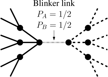
(b)

Figure 2: Schematic illustration of disordered configurations found with a majority rule dynamics on link states with no rewiring ($p=0$). a) Frozen disordered configuration. b) Dynamical trap based on a blinker link which keeps changing state forever with probability $1/2$.

In order to characterize the system at different times it is useful to consider the density of nodal interfaces $\rho$ as an order parameter Fernandez-Gracia2012 , defined as the fraction of pairs of connected links that are in different states. If $k_{i}$ is the degree of node $i$, and $k_{i}^{A/B}$ is the number of $A/B$-links connected to node $i$ (with obviously $k_{i}=k_{i}^{A}+k_{i}^{B}$), then $\rho$ is calculated as:

$$\rho=\frac{\sum_{i=1}^{N}k_{i}^{A}\,k_{i}^{B}}{\sum_{i=1}^{N}k_{i}(k_{i}-1)/2}.$$ (1)

The density $\rho$ is zero only when all connected links share the same state and it reaches its maximum value of $1/2$ for a random distribution of states (as it is the case in our initial condition), thus it is a measure of the local order in the system. Note that complete order, $\rho=0$, is achieved for both connected consensual configurations, where all links are in the same state, and configurations where the network is fragmented in a set of disconnected components, each formed by links with the same state. In both cases complete order is identified with absorbing configurations, where the system can no longer evolve. In terms of the node-equivalent graph, the line-graph, the order parameter $\rho$ becomes the density of active links, i.e., the fraction of links of the line-graph connecting nodes with different states.

III Final states

To explore how the coevolution of link states and network topology affects the final state of the system we run numerical simulations of the dynamics described above. The system evolves until the network reaches a final configuration that strongly depends on the system size $N$ and the rewiring probability $p$. The case $p=0$ corresponds to a static network situation, analyzed in Fernandez-Gracia2012 . In this case, system sizes larger than $N=500$ lead to disordered final states represented by network configurations composed by several interconnected clusters of type $A$ and $B$ links. A link that connects two clusters is either frozen, because it is in the local majority, or switching ad infinitum between states $A$ and $B$ (“blinking”), because it has the same number of neighboring links in each state. Therefore, we refer to these as disordered configurations ($\rho>0$) that are either frozen or dynamically trapped, respectively (see Fig. 2). For $p>0$ the network always reaches an absorbing ordered configuration that can be, either a one-component network with all links sharing the same state, or a fragmented network consisting of two large disconnected components of size similar to $N/2$ and in different states . We remark that all links inside each component are in the same state, thus the order parameter $\rho$ equals zero, as in the non-fragmented case. The behavior of $\rho$ for different values of $p$ is shown in Fig. 3, both as an average over different realizations (3b) and as single trajectories (3a). For $p=0$ almost every realization reaches a plateau or stationary value of $\rho>0$ (see Fig. 3a.1). For any $p>0$ every run reaches an ordered absorbing state with $\rho=0$ (see Figs. 3a.2, 3a.3). However, for small values of $p$ we observe a distinction between two groups of realizations, one ordering much faster than the other (see Fig. 3a.2). These different time scales will be discussed in section IV.

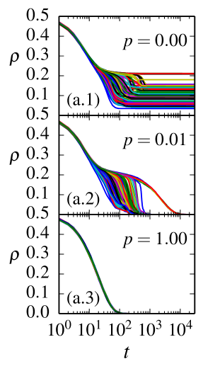
(a)

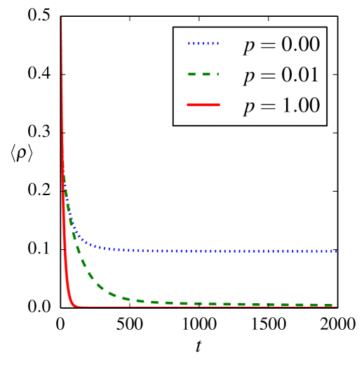
(b)

Figure 3: (Color online) Behavior of the order parameter for a system with $N=2000$ and $\langle k\rangle=10$. a) Density of nodal interfaces $\rho$ for $100$ individual realizations in linear-log scale. b) Average density of nodal interfaces $\langle\rho\rangle$ over $10000$ realizations. The time interval shown has been chosen for the sake of clarity; in reality, the runs for $p=0.01$ do not reach zero until $t\approx 30000$ while the ones for $p=1.00$ are zero from $t\approx 350$.

III.1 Fragmentation transition in finite systems

In order to explore how the network evolution affects the likelihood and the properties of the two possible outcomes, one component or fragmentation in two components, we study three relevant quantities. These are the probability $P_{1}$ that the final network is not fragmented, i.e, that it settles in one component, the relative size $s_{\scriptscriptstyle L}$ of the largest network component and the magnitude $\sigma_{s_{L}}$ of its associated fluctuations across different realizations.

Figure 4: (Color online) Probability $P_{1}$ that the system ends in a single network component vs the rewiring probability $p$, for networks of mean degree $\mu=10$ and size $N=500$ (circles), $N=1000$ (squares), $N=2000$ (triangles up), $N=4000$ (triangles left) and $N=8000$ (diamonds). $10000$ runs were used to estimate $P_{1}$, starting from an Erdös-Rényi network with random initial conditions. The limit of the region of bistability, $p^{*}$, is shown for the size $N=2000$. Note that $\forall p\geq p^{*},\;P_{1}(p)<1/N$. Inset: curves collapse when $p$ is rescaled by $N^{\alpha}$, with $\alpha=0.42$.

In Fig. 4 we show $P_{1}$ vs $p$, calculated as the fraction of simulation runs that ended up in a single component. We observe that $P_{1}=1$ only for $p=0$, then it decreases continuously between $p=0$ and a certain value $p=p^{*}$ and is always smaller than $1/N$ for $p\geq p^{*}$. This defines three regimes regarding $p$: one point at $p=0$ where the system is always connected, a region of bistability in $0<p<p^{*}$ where the system can both stay connected in one piece or break into disconnected components, and a fragmented region for $p\geq p^{*}$ where the network always splits apart.

Figure 5: (Color online) Average relative size $\langle s_{\scriptscriptstyle L}\rangle$ of the largest network component vs $p$, and for the same network sizes as in Fig. 4. $s_{\scriptscriptstyle L}$ is defined as the fraction of nodes included in the largest connected component. Inset: as in Fig. 4, $p$ is rescaled by $N^{\alpha}$, making the curves collapse to one.

Figure 6: (Color online) Standard deviation $\sigma_{s_{L}}$ of the relative size $s_{\scriptscriptstyle L}$ of the largest network component for the same system sizes $N$ as in Fig. 4. $\sigma_{s_{L}}$ is a measure of the magnitude of the fluctuations in the final size of the largest network component across different realizations of the dynamics. Inset: collapse of all curves by rescaling $p$ by $N^{\alpha}$ and $\sigma_{s_{L}}$ by $N^{-\beta}$, with $\alpha=0.42$ and $\beta=0.022$.

This result is consistent with the behavior of the average value of $s_{\scriptscriptstyle L}$ over many realizations (see Fig. 5), which decreases from $\langle s_{\scriptscriptstyle L}\rangle=1$ for $p=0$ to $\langle s_{\scriptscriptstyle L}\rangle\simeq 0.5$ for large $p$. As shown in Fig. 6, the standard deviation of $s_{\scriptscriptstyle L}$ ($\sigma_{s_{L}}$) has its maximum at a value $p_{\mbox{\tiny max}}$ for which $P_{1}$ is approximately $0.5$, that is, where fragmented and non-fragmented realizations are equally probable. The peak in $\sigma_{s_{L}}$ indicates a broad distribution of possible largest component sizes in that region and thus $p_{\mbox{\tiny max}}$ can be used as a footprint of the transition point. This broad distribution can also be seen in Fig. 7b, where we present a color-map of the fraction of runs that ended up in a given relative size $s_{\scriptscriptstyle L}$ of the largest network component for a network of $N=2000$ nodes. For the sake of clarity we also present in Fig. 7a histograms of network relative sizes $s$ (not only the largest) for four different values of $p$. We note that the maximum of $\sigma_{s_{L}}$ occurs around $p\approx 0.1$ (see Fig. 6), which corresponds in the color-map to a distribution of $s_{\scriptscriptstyle L}$ that has a peak at $s_{\scriptscriptstyle L}=1$ (one component) and a broad distribution corresponding to fragmented cases with $0.5\leq s_{\scriptscriptstyle L}\leq 0.875$. This division into fragmented and non-fragmented runs can also be clearly observed in the histogram corresponding to $p=0.1$ (see Fig. 7a.2).

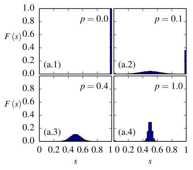
(a)

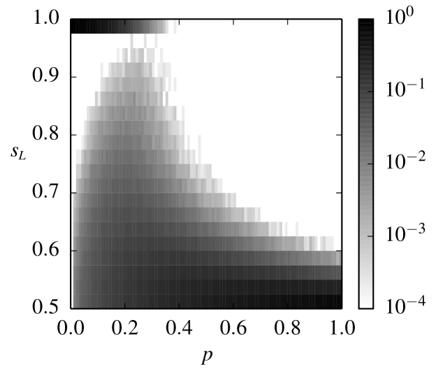
(b)

Figure 7: Relative sizes $s$ of network components for $N=2000$, $\langle k\rangle=10$ and $10000$ runs starting from random initial conditions. a) Histogram of network relative sizes for four different probabilities of rewiring $p$. b) Color-map of the fraction of runs ending in a given relative size of the largest network component $s_{\scriptscriptstyle L}$. Note the logarithmic color scale. White corresponds to no run ending in that relative size.

Interestingly, a common feature of $P_{1}(p)$, $s_{\scriptscriptstyle L}(p)$ and $\sigma_{s}(p)$ curves is that they are shifted to smaller values of $p$ as the system size $N$ increases, and thus the range of $p$ for which there is bistability of fragmented and non-fragmented outcomes seems to vanish in the thermodynamic limit, i.e., $p*$ tends to zero as size is increased. This shifting behavior also points at the fact that the transition point $p_{\mbox{\tiny max}}$ appears to tend to zero in the infinite size limit. A dependence of the transition point with the system size, in a way that it tends to zero in the infinite size limit, has been shown to be the case in several opinion dynamics models Toral2007 . Such systems, as it is the case here, do not display a typical phase transition in the thermodynamic limit with a well defined critical point and its associated critical exponents, divergences (in case of a continuous, second order phase transition) or discontinuities (in case of a first order phase transition). However, for any finite system a transition point can be clearly defined as separating two different behavioral regimes.

To gain an insight about the $N\to\infty$ behavior, we perform a finite size scaling analysis by assuming that $P_{1}$, $s_{\scriptscriptstyle L}$ and $\sigma_{s_{L}}$ are functions of the variable $x\equiv p\,N^{\alpha}$:

$$P_{1}(p,N) =P_{1}(p\,N^{\alpha}),$$ (2)

$$s_{\scriptscriptstyle L}(p,N) =s_{\scriptscriptstyle L}(p\,N^{\alpha}),$$

$$\sigma_{s_{L}}(p,N) =N^{\beta}\sigma_{s_{L}}(p\,N^{\alpha}).$$

The values of the exponents $\alpha$ and $\beta$ should be such that make the curves for different sizes collapse into a single curve. Therefore, the location of the peak in all $\sigma_{s_{L}}(p)$ curves of Fig. 6 should scale as $p_{\mbox{\tiny max}}\sim N^{-\alpha}$. By fitting a power law function to the plot $p_{\mbox{\tiny max}}$ vs $N$ we found $\alpha\simeq 0.42$ (not shown). In the insets of Figs. 4, 5 and 6 we observe the collapse for different network sizes when magnitudes are plotted versus the rescaled variable $x$ (rescaling also the y-axis by $N^{-\beta}$ in the case of $\sigma_{s_{L}}$). This scaling analysis shows that, in the thermodynamic limit, the network would break apart for any finite value of $p>0$. This might be related to the fact that when the system evolves under the majority rule alone, it always gets trapped in disordered configurations (in the $N\to\infty$ limit). Then, it seems that even a very small rewiring rate is enough to remove the system from traps, but at the cost of breaking the network apart. However, as we will show in the next section, the time needed for the fragmentation to occur diverges with system size. A deeper understanding of this phenomenon can be achieved by studying stochastic trajectories of single realizations.

IV Time evolution

We are interested in quantifying the evolution of the system towards the final states described above. In Fig. 8 we plot the survival probability $P_{s}(t)$, i.e, the probability that a realization did not reach the ordered state ($\rho=0$) up to time $t$.

Figure 8: (Color online) Time evolution of the survival probability $P_{s}$ for different values of $p$ and networks of size $N=500$, $1000$, $2000$, $4000$ and $8000$ (curves from bottom to top and, respectively, dotted, dashed, dash-dotted, solid and dash-dash-dotted). Averages are over $10^{4}$ independent runs.

When $p=0$ we have $P_{s}=1$ for all times, meaning that all realizations (except for a few runs with the smallest size $N=500$, as reported in Fernandez-Gracia2012 ) fall into a disordered configuration characterized by a constant value of $\rho>0$, as we shall discussed in detail in the next section. For $p=0.01$, $p=0.05$ and $p=0.10$ [Figs. 8(a), 8(b) and 8(c), respectively] we observe that $P_{s}$ experiences two decays at very different time scales, revealing the existence of two different ordering mechanisms. As we will explain, the first decay from $P_{s}=1$ to a plateau corresponds to the ordering of non-fragmented realizations, while the second decay from the plateau to zero is due to the ordering of fragmented runs. Take, for instance, $p=0.01$ and $N=8000$. We observe in Fig. 4 that the fraction of runs ending in one component is $P_{1}\simeq 0.9$. We interpret that it is the arrival of this $90\%$ of runs to a one-component absorbing state with $\rho=0$ which produces the first decay of the survival probability to $P_{s}\simeq 0.1$ around a time $t\simeq 10^{3}$, as can be observed in Fig. 8(a). The remaining fraction $P_{s}\simeq 0.1$ that survive lead to the plateau that lasts up to the second decay around $t\simeq 10^{4}$, when they arrive to a fragmented absorbing state again with $\rho=0$. Note also that both decay times decrease for increasing $p$, while the height of the plateau rises ($P_{1}$ increases). In the $p=0.30$ case [Fig. 8(d)] the first decay of $P_{s}$ is only observed for small systems, since for larger ones most realizations end up with a fragmented network (see Fig.4). This picture also holds for larger values of $p$.

IV.1 Description of trajectories in phase space

In order to gain an insight about the fragmentation phenomenon, we investigate in this section individual trajectories of the system on the $m-\rho$ plane, where $m$ is the link magnetization Vazquez2008a ; Vazquez2008b , the difference between the fractions of $A$ and $B$ links,

$$m=\frac{\sum_{i=1}^{N}\left(k_{i}^{A}-k_{i}^{B}\right)}{\sum_{i=1}^{N}k_{i}}.$$ (3)

In Fig. 9 we display typical trajectories of the system for a network of $N=2000$ nodes and values of the rewiring probability $p=0,0.01,0.1$ and $0.5$. Trajectories start at $(m,\rho)\simeq(0,0.5)$, corresponding to random initial conditions. Points $(1,0)$ and $(-1,0)$ represent $A$ and $B$ one-component consensual configurations, while the absorbing line $\rho=0$ with $|m|<1$ corresponds to a fragmented network.

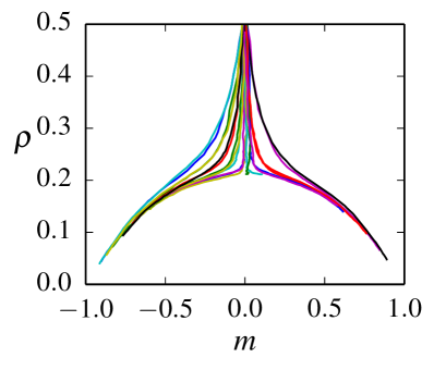
(a) $p=0.00$

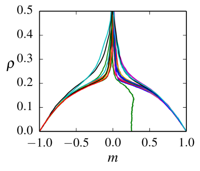
(b) $p=0.01$

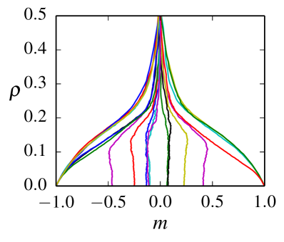
(c) $p=0.10$

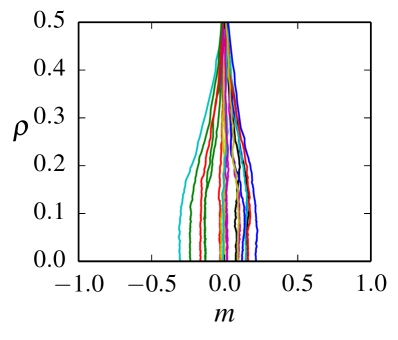
(d) $p=0.50$

Figure 9: (Color online) Typical trajectories of the system on the $(m,\rho)$ space for a network of $N=2000$ nodes and different values of the rewiring probability $p$.

In the $p=0$ case (Fig. 9a), we observe that realizations undergo a fast initial ordering in which associated trajectories go from $\rho\simeq 0.5$ to $\rho\simeq 0.2$ (with some small changes in $m$) in approximately $25$ Monte Carlo steps. This corresponds to the fast formation of two giant (connected) domains of opposite states due to the majority rule dynamics, as has been reported in previous works Castellano2006 . Afterwards trajectories enter in a common curve which, as in other cases Vazquez2008a , can be fit by a parabola and where the ordering process is accompanied by a change in magnetization. In our case the parabola takes the approximate form $\rho\simeq 0.2(1-m^{2})$ and the system evolves following a direct path towards $|m|=1$, due to the fact that $\rho$ cannot increase in a majority rule update. This corresponds to the largest domain progressively invading the other. However, the ordering stops abruptly when the system falls to a topologically trapped state with $\rho>0$, preventing it from arriving to the one-component ordered $A$ or $B$ states, $(1,0)$ or $(-1,0)$ points, respectively.

For $p=0.01$ (Fig. 9b) most runs finally arrive to the one-component ordered state, by means of the rewiring mechanism that helps the system escape from frozen or dynamical traps. As mentioned before, even a small rewiring rate is able to unlock frustrated links, allowing the system to keep evolving towards one-component order ($|m|=1$, $\rho=0$). Nevertheless, there are some runs that escape from the parabola and follow a nearly vertical downward trajectory (line ending at $\rho=0$ and $m\simeq 0.25$), even if they are initially attracted towards $|m|=1$. These runs are trapped around a given value of $m$ and experience a relaxation that decreases $\rho$ very slowly while keeping $m$ almost constant. It seems that in these realizations some rewiring events trigger only a few successful majority rule updates that are not enough to completely order the system in a one-component network. This corresponds to the process of fragmentation of the network in two components with different states. For larger rewiring rates more runs end up fragmenting in two components (see Fig. 9c), until for large enough $p$ no run is able to follow the parabola (see Fig. 9d), leading to only fragmented final states.

IV.2 Mean-field approach

As explained in the last section and shown in Fig. 3, $\langle\rho\rangle$ undergoes a first fast decay in a short time scale corresponding to the contribution of non-fragmented realizations, and then a second much slower decay that corresponds to fragmented realizations. Therefore, bearing in mind that much of the time evolution of $\langle\rho\rangle$ is controlled by the second very slow dynamics of fragmenting realizations, we develop in this section an analytical approach for this second regime. We assume that the system starts at $t=0$ from a trapped configuration (see Fig. 2), which consists of two network components of similar size $N/2$ interconnected by frustrated links. These are links with the same state as the majority of their neighboring links, thus they cannot change state (see Fig. 2a), or links with equal number of neighbors in each state, thus they keep flipping state from $A$ to $B$ and vice versa (blinkers, see Fig. 2b). To estimate how the density of frustrated links $\beta$ varies with time, we now describe the events and their associated probabilities that lead to a change in $\beta$. In a single time step of interval $dt=1/N$, a frustrated link is chosen with probability $\beta$. Then, with probability $p/2$ the end of the link connected to the minority is randomly chosen and rewired to another random node in the network. Finally, this end lands on the component that holds the link’s state with probability $1/2$. After the rewiring this link is no longer connecting components, thus the number of frustrated links is reduced by $1$, leading to a change $\Delta\beta=-2/\mu N$ (with $\mu\equiv\langle k\rangle$, as above). Assembling all these factors, the average density of frustrated links evolves according to

$$\frac{d\beta(t)}{dt}=-\frac{p}{2\mu}\beta(t),$$ (4)

with solution

$$\beta(t)=\beta_{0}\,e^{-\frac{p}{2\mu}t},$$ (5)

where $\beta_{0}$ is the initial density of frustrated links. Given that, on average, each frustrated link accounts for the existence of $\mu-1$ nodal interfaces, $\rho$ is proportional to $\beta$, and therefore we expect that the average density of interfaces decays as

$$\rho(t)\sim e^{-\frac{p}{2\mu}t}.$$ (6)

Figure 10: (Color online) Time evolution of the average density of nodal interfaces $\langle\rho\rangle$ on a linear-log scale, for values of the rewiring probability $p$ as indicated in the box. Symbols at the top correspond to simulations on a network of $N=4000$ nodes and mean degree $\mu=20$, while bottom symbols are for a network of size $N=8000$ and mean degree $\mu=10$. Time is rescaled by $p$ and $\langle\rho\rangle$ is normalized by its initial value to make the data collapse. Solid lines are the analytical approximations from Eq. (6).

In Fig. 10 we show $\langle\rho\rangle$ vs time obtained from numerical simulations for various values of $p$ (symbols) and two different networks, one of size $N=8000$ and $\mu=10$ and the other with $N=4000$ nodes and $\mu=20$. We observe that the expression (6) (solid lines) captures the behavior of $\langle\rho\rangle$ for most values of $p$ and has the correct scaling with $\mu$. The data for $p=0.2$ deviates from the pure exponential decay at long times, probably because the analytical approximation works better for large $p$, where the rewiring process seems to dominate the dynamics.

IV.3 Convergence times

Another quantity that is worth studying in this system is the time to reach the final state, or convergence time, given that it complements our previous analysis of the two ordering dynamics, majority rule and rewiring. In Fig. 11 we show the mean time of convergence to the final ordered state for non-fragmented and fragmented runs $T_{1}$ and $T_{2}$, respectively, versus the rewiring probability $p$ . Results are shown for three different system sizes. We observe that $T_{2}$ is about ten times larger than $T_{1}$ for all values of $p$. This confirms the dynamical picture that we discussed in the previous sections. There is a first fraction of runs in which the majority rule dynamics plays a leading role constantly ordering the system until it reaches one-component full order in a short time scale $T_{1}$. But there is also a second fraction which fall into particular topological traps that prevent the system to keep ordering, and then the rewiring process slowly leads to the fragmentation of the network in a much longer time scale $T_{2}$. Interestingly, rewiring always works as a perturbation that frees the system whenever it gets trapped, but it seems that in the first type of runs perturbations trigger cascades of ordering updates which are large enough to completely order the network before it breaks apart.

Figure 11: (Color online) Mean time to reach the fragmented and non-fragmented final states $T_{1}$ and $T_{2}$, respectively, vs the rewiring probability $p$, for networks of size $N=500$ (circles), $N=2000$ (squares) and $N=8000$ (diamonds), and mean degree $\mu=10$. The inset shows the scaling of $T_{2}$ as described by Eq. (7).

An approximate expression for $T_{2}$ can be obtained by considering the relaxation to the fragmented state given by Eq. (6), where the mean number of nodal interfaces decreases to zero. The network breaks in two components when the fraction of frustrated links holding both components together becomes smaller than $2/\mu N$, or $\rho\sim 1/N$, since $\rho$ is proportional to $\beta$, as we mentioned before. Then, we can write $1/N\sim\exp(-p\,T_{2}/2\mu)$, from where

$$T_{2}\sim\frac{\mu}{p}\ln N.$$ (7)

The inset of Fig. 11 shows that the approximate expression (7) captures the right scaling of $T_{2}$ with $p$ and $N$. In Fig. 12 we check the dependence of $T_{1}$ and $T_{2}$ with the system size $N$. The y-axis of the main plot showing $T_{2}$ was rescaled according to Eq. (7). The inset shows that $T_{1}$ also scales as $\ln N$.

Figure 12: (Color online) Convergence times $T_{1}$ and $T_{2}$ vs system size $N$ for $p=0.1$ and $\mu=10$. Main: y and x-axis were rescaled according to Eq. (7). Inset: data is shown on a log-linear scale. The solid line is the best fit $T_{1}=30.7\,\ln N-84.5$.

As Fig. 11 shows, both $T_{1}$ and $T_{2}$ decay as $1/p$ in the low $p$ limit. This is because when $p$ is very small we can picture a typical evolution of the system as a series of alternating pinning and depinning processes. That is, initially a series of majority rule updates take place, which partially order the system until it reaches a frustrated configuration. Then the system stays trapped there for a time of order $1/p$ until a successful rewiring event unlocks it. This is followed by another avalanche of majority rule updates that ends on the next trapped state. This process is repeated until a final absorbing ordered configuration is reached. Given that the mean time interval between two avalanches scales as $1/p$, the convergence time to any final state should scale as $1/p$ (see Fig. 11). This implies that $T_{1}$ and $T_{2}$ diverge as $p\to 0$. However, when $p$ is strictly zero the system is absorbed in a disordered configuration, which can be frozen or dynamically trapped, and so the convergence time is finite. The $p=0$ case also differs from the $p>0$ case in the fact that convergence times to the absorbing disordered configurations seem to scale as $T\sim N^{0.375}$ (see Fig. 13), instead of $\ln N$.

Figure 13: (Color online) Average time to reach an absorbing disordered state $T$ vs systems size $N$ on a double logarithmic scale, for a static network ($p=0$). The dashed line has slope $0.375$. The log-linear scale in the inset shows that $T$ grows faster than $\ln N$.

V Summary and Conclusions

We have studied a model that explores the majority rule link dynamics on a coevolving network, where links in the local minority are rewired at random. On topologically static ($p=0$) large networks, the ordering process induced by the majority rule stops before a completely ordered state is reached with all links in the same state (the only possibility with no rewiring), because the system falls into trapped disordered configurations. When the rewiring is switched on ($p>0$), the system is able to escape from these trapped configurations and reach an ordered absorbing state that can be either a one-component network with all links in the same state or a fragmented network with two opposed states disconnected components. The former output is more likely when the rewiring rate is low or networks are small, while the latter output becomes more and more common as the rewiring rate increases or networks get larger, and it is the only possible result for large rewiring rates or in the limit of very large networks. For any finite size network, a range of values of the rewiring probability $p$ can be found for which there is bistability between both possible outcomes. In the very large size limit, however, the bistability region progressively vanishes and thus even very small amounts of rewiring make the network break apart.

By studying the trajectories of the system in the $m-\rho$ space we were able to identify two types of evolutions, which provides an insight about the mechanism of fragmentation. For no rewiring, all trajectories fall into an attractive path with a parabolic envelope that ends in a point corresponding to a one-component ordered configuration. However, these trajectories stop before reaching that point, indicating that the system is trapped in a disordered configuration. For low rewiring, most trajectories quickly move along the parabola until they hit the one-component ordered absorbing point. This complete ordering process is mainly driven by majority rule updates, and happens in a quite short time scale. For high rewiring a new scenario appears. Most trajectories quickly stop at some point in the parabola, and then slowly follow a nearly vertical path that ends in the absorbing line $\rho=0$ with $|m|<1$, corresponding to a fragmented network. This second fragmentation process takes a much longer time than the initial ordering process, and controls the total convergence time to the final state.

Our results show that the frozen and dynamically trapped disordered configurations promoted by the link-based majority rule dynamics are not robust against topological perturbations in the form of a rewiring, since the continuous relinking updates are able to remove the system from the topological traps. However, if instead of topological perturbations we consider perturbations on the state dynamics in the form of a temperature, as in a Glauber dynamics with a non-zero temperature, we find that the frozen and dynamically trapped configurations appear to be robust for small noise intensities . Indeed, even if any finite system with finite temperature perturbations is expected to order by finite-size fluctuations, the ordering times become so large even for small systems that, in practice, one can consider them as permanently trapped in a disordered configuration.

By adopting a link-state perspective, our research contributes to the understanding of complex phenomena emerging from the coupling of diffusive processes with time varying networks. However, both reference Fernandez-Gracia2012 and this paper are limited to states defined on the links. A natural step further would be to consider mixed dynamics, with states defined both on the nodes and on the links and a certain coupling between them. Continuing with the language competition example used above, the node dynamics would correspond to the evolution of language competence or preference, while the dynamics on the links would mimic the evolution of language use. Work along these lines is in progress.

- (1) C. Castellano, S. Fortunato, and V. Loreto, Rev. Mod. Phys. 81, 591 (2009)
- (2) F. Heider, The Journal of Psychology 21, 107 (1946)
- (3) T. Antal, P. L. Krapivsky, and S. Redner, Phys. Rev. E 72, 036121 (2005)
- (4) T. Antal, P. Krapivsky, and S. Redner, Physica D: Nonlinear Phenomena 224, 130 (2006)
- (5) F. Radicchi, D. Vilone, S. Yoon, and H. Meyer-Ortmanns, Phys. Rev. E 75, 026106 (2007)
- (6) M. Szell, R. Lambiotte, and S. Thurner, Proceedings of the National Academy of Sciences 107, 13636 (2010)
- (7) J. Leskovec, D. Huttenlocher, and J. Kleinberg, in Proceedings of the 19th International Conference on World Wide Web, WWW ’10 (ACM, New York, NY, USA, 2010) pp. 641–650
- (8) J. Leskovec, D. Huttenlocher, and J. Kleinberg, in Proceedings of the SIGCHI Conference on Human Factors in Computing Systems, CHI ’10 (ACM, New York, NY, USA, 2010) pp. 1361–1370
- (9) S. A. Marvel, J. Kleinberg, R. D. Kleinberg, and S. H. Strogatz, Proceedings of the National Academy of Sciences 108, 1771 (2011)
- (10) V. A. Traag and J. Bruggeman, Phys. Rev. E 80, 036115 (2009)
- (11) T. S. Evans and R. Lambiotte, Phys. Rev. E 80, 016105 (2009)
- (12) T. S. Evans and R. Lambiotte, The European Physical Journal B 77, 265 (2010)
- (13) Y.-Y. Ahn, J. P. Bagrow, and S. Lehmann, Nature 466, 761 (2010)
- (14) D. Liu, N. Blenn, and P. V. Mieghem, Procedia Computer Science 9, 1400 (2012), proceedings of the International Conference on Computational Science, ICCS ’12
- (15) S. Fortunato, Physics Reports 486, 75 (2010)
- (16) T. Nepusz and T. Vicsek, Nature Physics 8, 568 (2012)
- (17) J. Fernández-Gracia, X. Castelló, V. M. Eguíluz, and M. San Miguel, Phys. Rev. E 86, 066113 (2012)
- (18) A. Rooij and H. Wilf, Acta Mathematica Academiae Scientiarum Hungarica 16, 263 (1965)
- (19) M. Krawczyk, L. Muchnik, A. Mańka-Krasoń, and K. Kulakowski, Physica A: Statistical Mechanics and its Applications 390, 2611 (2011)
- (20) G. Chartrand and M. Stewart, Mathematische Annalen 182, 170 (1969)
- (21) A. Mańka-Krasoń, A. Mwijage, and K. Kulakowski, Computer Physics Communications 181, 118 (2010)
- (22) T. Gross and B. Blasius, Journal of The Royal Society Interface 5, 259 (2008)
- (23) J. L. Herrera, M. G. Cosenza, K. Tucci, and J. C. González-Avella, Europhys. Lett. 95, 58006 (2011)
- (24) H. Sayama, I. Pestov, J. Schmidt, B. J. Bush, C. Wong, J. Yamanoi, and T. Gross, Computers & Mathematics with Applications 65, 1645 (2013)
- (25) M. G. Zimmermann, V. M. Eguíluz, and M. San Miguel, in Economics with Heterogeneous Interacting Agents, Lecture Notes in Economics and Mathematical Systems, Vol. 503, edited by A. Kirman and J.-B. Zimmermann (Springer Berlin Heidelberg, 2001) pp. 73–86
- (26) M. G. Zimmermann, V. M. Eguíluz, and M. San Miguel, Phys. Rev. E 69, 065102 (2004)
- (27) P. Holme and M. E. J. Newman, Phys. Rev. E 74, 056108 (2006)
- (28) F. Vazquez, J. C. González-Avella, V. M. Eguíluz, and M. San Miguel, Phys. Rev. E 76, 046120 (2007)
- (29) F. Vazquez, V. M. Eguíluz, and M. San Miguel, Phys. Rev. Lett. 100, 108702 (2008)
- (30) S. Mandrà, S. Fortunato, and C. Castellano, Phys. Rev. E 80, 056105 (2009)
- (31) G. Demirel, F. Vazquez, G. Böhme, and T. Gross, Physica D: Nonlinear Phenomena 267, 68 (2014)
- (32) O. Häggström, Physica A: Statistical Mechanics and its Applications 310, 275 (2002)
- (33) C. Castellano, V. Loreto, A. Barrat, F. Cecconi, and D. Parisi, Phys. Rev. E 71, 066107 (2005)
- (34) C. Castellano and R. Pastor-Satorras, Journal of Statistical Mechanics: Theory and Experiment 2006, P05001 (2006)
- (35) Y. Baek, M. Ha, and H. Jeong, Phys. Rev. E 85, 031123 (2012)
- (36) D. M. Abrams and S. H. Strogatz, Nature 424, 900 (2003)
- (37) X. Castelló, V. M. Eguíluz, and M. San Miguel, New Journal of Physics 8, 308 (2006)
- (38) M. Patriarca, X. Castelló, J. R. Uriarte, V. M. Eguíluz, and M. San Miguel, Advances in Complex Systems 15, 1250048 (2012)
- (39) X. Castelló, L. Loureiro-Porto, and M. San Miguel, International Journal of the Sociology of Language, 21–51(2013)
- (40) Different implementations are possible, for example, by varying the probability to switch states in case of tie.
- (41) A few disconnected nodes can also be occasionally found.
- (42) R. Toral and C. J. Tessone, Commun. Comput. Phys. 2, 177 (2007)
- (43) F. Vazquez and V. M. Eguíluz, New Journal of Physics 10, 063011 (2008)
- (44) Here the subindices and refer to one and two components, even though fragmented runs may also have a few disconnected nodes
- (45) A. Carro, M. San Miguel, R. Toral, unpublished.