On the fine structure of the Cepheid metallicity gradient in the Galactic thin disk

We present homogeneous and accurate iron abundances for 42 Galactic Cepheids based on high–spectral resolution (R$\sim$ 38,000) high signal-to-noise ratio (SNR $\geq$ 100) optical spectra collected with UVES at VLT (128 spectra). The above abundances were complemented with high–quality iron abundances provided either by our group (86) or available in the literature. We paid attention in deriving a common metallicity scale and ended up with a sample of 450 Cepheids. We also estimated for the entire sample accurate individual distances by using homogeneous near-infrared photometry and the reddening free Period-Wesenheit relations. The new metallicity gradient is linear over a broad range of Galactocentric distances ($R\rm_{G}\sim$5–19 kpc) and agrees quite well with similar estimates available in the literature (-0.060$\pm$0.002 dex/kpc). We also uncover evidence which suggests that the residuals of the metallicity gradient are tightly correlated with candidate Cepheid Groups (CGs). The candidate CGs have been identified as spatial overdensities of Cepheids located across the thin disk. They account for a significant fraction of the residual fluctuations, and in turn for the large intrinsic dispersion of the metallicity gradient. We performed a detailed comparison with metallicity gradients based on different tracers: OB stars and open clusters. We found very similar metallicity gradients for ages younger than 3 Gyrs, while for older ages we found a shallower slope and an increase in the intrinsic spread. The above findings rely on homogeneous age, metallicity and distance scales. Finally we found, by using a large sample of Galactic and Magellanic Cepheids for which are available accurate iron abundances, that the dependence of the luminosity amplitude on metallicity is vanishing.

1 Introduction

Recent findings concerning the metallicity gradient across the Galactic thin disk, based on high spectral resolution, high signal-to-noise spectra and on stellar tracers for which we can provide accurate individual Galactocentric distances, are disclosing a new interesting scenario. The iron gradients traced by stellar populations younger than a few hundred of Myrs show a well defined trend when moving from the inner to the outer disc regions. The iron abundances in the innermost disc regions ($R_{G}\sim$5 kpc) are well above solar ([Fe/H]$\sim$0.4, Andrievsky et al., 2002b; Pedicelli et al., 2009; Luck et al., 2011; Luck & Lambert, 2011; Genovali et al., 2013, hereinafter G13) while in the outer disk ($R_{G}\sim$15 kpc) they are significantly more metal–poor ([Fe/H]$\sim$-0.2/-0.5, Andrievsky et al., 2004; Yong et al., 2006; Lemasle et al., 2008). However, the young stellar populations in the two innermost Galactic regions showing ongoing star formation activity –the Bar and the Nuclear Bulge– attain solar iron abundances. Thus suggesting that the above regions are experiencing different chemical enrichment histories (Bono et al., 2013).

The use of high-quality data and homogeneous analysis of large sample of classical Cepheids and young massive main sequence stars provided the opportunity to overcome some of the systematics affecting early estimates of the metallicity gradient. However, current findings still rely on several assumptions that might introduce systematic errors.

i) Distances – Cepheids are very solid primary distance indicators, but they only trace young stellar populations. The use of red clump stars is very promising, since they are ubiquitous in the innermost Galactic regions. However, their individual distances might be affected by larger uncertainties, since we are dealing with stellar populations covering a broad range in ages and in metal abundances (Girardi & Salaris, 2001; Salaris & Girardi, 2002).

ii) Gradients – Recent spectroscopic investigations indicate that the use of homogeneous and accurate iron abundances decreases the spread along the radial gradient (G13). This means that they can be adopted to investigate the fine structure of the metallicity distribution (Lépine et al., 2011) and the possible occurrence of gaps and/or of changes in the slope (Lépine et al., 2013).

iii) Ages – The central helium burning phases of intermediate–mass ($M\sim$3.5–10 $M_{\odot}$) stars take place along the so–called blue loops. During these phases an increase in stellar masses causes a steady increase in the mean luminosity. These are the reasons why classical Cepheids do obey to a Period-Age relation. However, the ages covered by Cepheids is quite limited ($\approx$20–400 Myr). Most of the current chemical evolution models do predict a steady decrease in slope of the metallicity gradient as a function of age (Portinari & Chiosi, 2000; Cescutti et al., 2007; Minchev et al., 2013). However, we still lack firm estimates of this effect since homogeneous estimates of distance, age and chemical composition for a large sample of intermediate and old open clusters (Salaris et al., 2004; Carraro et al., 2007b; Yong et al., 2012) are still missing.

In this investigation we provide new accurate and homogeneous iron abundance estimates for 42 Galactic Cepheids based on high spectral resolution, high signal-to-noise ratio ($S/N$) spectra acquired with UVES at VLT. The total sample includes estimates for 75 Cepheids (74 Classical Cepheids and one Type II Cepheid –DD Vel– that will be discussed in a forthcoming paper), whose abundances were partially published in Genovali et al. (2013). Moreover, we also analyzed three high spectral resolution spectra for the Cepheids –TV CMa, RU Sct, X Sct– collected with NARVAL at the Télescope Bernard Lyot (TBL) that we adopted to double check current iron abundance estimates. We also added a new estimate of the FEROS spectrum for the Cepheid CE Pup whose metallicity was already available in the literature (Luck et al., 2011).

The above iron abundances were complemented with similar estimates provided either by our group (Lemasle et al., 2007; Lemasle et al., 2008; Romaniello et al., 2008, 53 Cepheids) or available in the literature (Yong et al., 2006; Luck et al., 2011; Luck & Lambert, 2011, 322 Cepheids). We ended up with a sample of 450 Classical Cepheids i.e. the 73% of the entire sample of known Galactic Cepheids according to the Classical Cepheids list in the GCVS (candidate Cepheids are excluded from this estimate). For the entire sample, we estimated homogeneous distances based on reddening-free near infrared Period–Wesenheit relations (Inno et al., 2013).

This is the eighth paper of a series devoted to chemical composition of Galactic and Magellanic Cepheids (see the reference list). The name of the project is DIsk Optical and Near infrared Young Stellar Object Spectroscopy (DIONYSOS). The structure of the paper is the following. In §2 we present the spectroscopic data sets adopted in the current investigation and the method adopted to estimate the iron abundances. The photometric data and the individual distances are discussed in §3, together with a detailed analysis of the errors affecting Cepheid distances. §4 deals with the metallicity gradient, while in §5 we investigate the dependence of the metallicity gradient on stellar age. In this section the metallicity gradient is compared with the metallicity gradients based on younger tracers (OB stars) and with intermediate-age tracers (open clusters). In §6 we address in detail the fine structure of the metallicity gradient and perform a thorough analysis of the Cepheid radial distribution across the Galactic disk. §7 deals with the longstanding open problem concerning the dependence of the luminosity amplitude on the metallicity, while in §8 we summarize the results and briefly outline the future developments of this project.

2 Spectroscopic data and iron abundances

2.1 Spectroscopic data

In this investigation we present a spectral analysis based on high-resolution (R$\sim$38,000) spectra collected with the UVES spectrograph available at the Nasmyth B focus of UT2/VLT Cerro Paranal telescope. Multi–epoch spectra for eleven Galactic Cepheids were collected during observing run B (P89). This sample includes 44 high-resolution spectra (from four to six spectra per star) for a total of eleven Cepheids. The covered spectral range is 4726–5804 Å and 5762–6835 Å over the two chips, collected by only using the red arm configuration and the cross disperser CD#3 (central wavelength at 580 nm). The $S/N$ ranges from $\sim$50 to $\sim$300 (see Fig. 1). The seeing during the observations was ranging from 0.5 to 2.5 arcsec, with a typical mean value of 1.2 arcsec, while the exposure times changed from 20 to 1400 sec.

We make use of an additional UVES sample partially presented in G13. The spectra were collected at random pulsational phases between 2008 October and 2009 April using the DIC2 (437+760) configuration with blue and red arms operating in parallel. The two arms cover the wavelength intervals $\sim$3750–5000 Å and $\sim$5650–7600/7660–9460 Å (two chips in the red arm). The exposure time ranges from 80 to 2000 sec, while the seeing ranges from 0.6 to 2 arcsec with a mean value of 1.2 arcsec. The $S/N$ is typically better than $\sim$100 for all the echelle orders. The complete spectroscopic sample includes 84 spectra for a total of 77 Cepheids. The spectra of three Cepheids –WW Mon, V641 Cen, GQ Ori– were analyzed, but they were not included in the abundance analysis because the SNR ratio of the individual spectra was not good enough. The entire sample of UVES spectra were reduced using the ESO UVES dedicated pipeline REFLEX v2.1 (Ballester et al., 2011).

For three Cepheids –TV CMa, RU Sct, X Sct– we also analyzed high $S/N$ spectra collected with NARVAL at TBL. NARVAL has a spectral resolution of $\sim$75,000 and covers the wavelength range 3700-10500 Å. The NARVAL spectra were reduced using the data reduction software Libre-ESpRIT, written by Donati. We also included the re-analysis of a FEROS spectrum for CE Pup (Luck et al., 2011) to better constrain possible systematic differences in the metallicity estimates of the outer disk.

As a whole, we provide in this investigation an updated spectroscopic estimate of the iron abundance for 42 Classical Cepheids located either in the outer disk or in the solar neighbourhood. Together with the iron abundances provided by G13 we ended up with a homogeneous metallicity sample for 74 Classical Cepheids.

2.2 Method

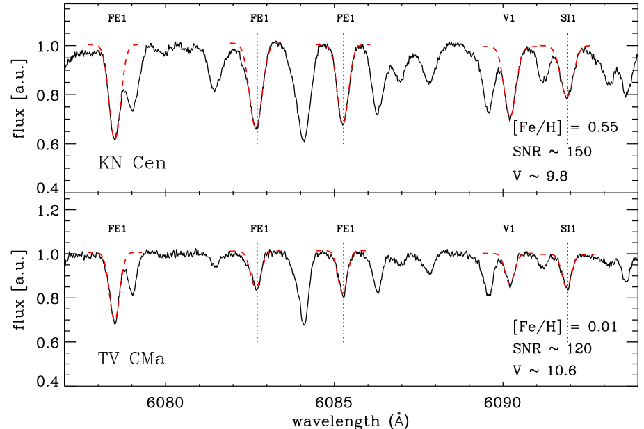
Figure 2: High-resolution (R$\sim$38,000) UVES spectrum of KN Cen ([Fe/H] $=0.55\pm 0.12$, Genovali et al. 2013) and TV CMa ([Fe/H] $=0.01\pm 0.07$, Genovali et al. 2013). The apparent visual magnitude and the SNR in the spectral range $\lambda$ $\sim$ 5650 - 7500 Å (red arm) are also labeled. The vertical dashed lines display selected lines (Fe I 6078.50, Fe I  6082.72, Fe I 6085.27, V I 6090.21, Si I 6091.92 Å) adopted to estimate the individual $T\rm_{eff}$ with the LDR method (Kovtyukh & Gorlova, 2000) (red dashed lines).

We implemented a dedicated semi-automatic procedure able to determine the continuum and to fit the line profile by single or double Gaussian functions (see Fig. 2), depending on the line blending. We adopted the iron linelist presented in Genovali et al. (2013) and typically we measured the equivalent width (EW) of $\sim$ 100 - 200 Fe I and $\sim$ 20 - 40 Fe II lines, depending on the specific spectral range.

The abundance determination was performed by using the code calrai originally developed by Spite (1967) and continuously updated since then. Once fixed the atmospheric parameters, the code performs an interpolation over a grid of LTE, plane-parallel atmosphere models (MARCS, Gustafsson et al, 2008) and provides [Fe/H] and its intrinsic error. The abundances of the other elements will be discussed in a forthcoming paper.

For each spectrum we computed the curves of growth for both neutral and ionized iron. The process is iterated until a good match between the predicted and observed equivalent widths (and thus the curves of growth) is obtained.

The effective temperature –$T_{eff}$– for individual spectra was independently estimated by using the line depth ratio (LDR) method (Kovtyukh & Gorlova 2000). Typically, we measured two dozen of LDRs per spectrum (see e.g. Fig. 2). The estimated $T_{eff}$ was validated by ensuring that $Fe\,{\scriptsize I}$ does not depend on the excitation potential ($\chi_{ex}$) i. e. the slope of Fe Ivs $\chi_{ex}$ is minimal. The surface gravity –log g– was derived by imposing the ionization balance between Fe Iand Fe II. The micro-turbulent velocity –vt– was estimated by minimizing the $Fe\,{\scriptsize I}$ vs EW slope. The atmospheric parameters estimated for each spectrum are given in Table LABEL:tab:table_atm_par.

The maximum EW value included in the analysis varies according to the metallicity itself and on the atmospheric parameters of the star. For a large fraction of our spectra we were able to use only relatively weak lines (EW $\leq$ 120 mÅ) located along the linear part of the curve of growth. In a few cases the spectra were lacking of a significant number of weak lines (less than two Fe II lines), therefore, we included in the analysis also lines with EW up to 180 mÅ. The latter ones cause a mild increase in the uncertainties affecting the correlated atmospheric parameters and become of the order of $\Delta$log $g$ 0.3 dex and $\Delta$$v_{t}$ 0.5 km/s. The impact that typical uncertainties on effective temperature, surface gravity and microturbulent velocity have on the mean iron abundance are listed in Table 2. Data given in this table indicate that the difference in iron is on average smaller than 0.2 dex. Moreover, the difference in iron does not seem to depend, within the uncertainties, on the pulsation phase.

The mean iron abundances given in column 8 of Table LABEL:tab:tab_distances are the weighted mean of [Fe I/H] and [Fe II/H] with associated errors, i.e. $\sigma_{Fe}$=$\sqrt{\sigma_{Fe\,{\scriptsize I}}^{2}+\sigma_{Fe\,{\scriptsize II}}^{2}}$, where $\sigma_{Fe\,{\scriptsize I}}$ and $\sigma_{Fe\,{\scriptsize II}}$ are the standard deviations of [Fe I/H] and [Fe II/H] estimates given by the lines measured in a single spectrum. For Cepheids in our sample with multiple measurements the weighted average abundance and the standard deviation $\sigma_{Fe}$=$\sqrt{\sum_{i}\sigma_{Fe,i}^{2}}$ are also listed. The iron abundances were estimated by assuming the solar iron abundance provided by Grevesse et al. (1996), i.e. A(Fe)_⊙ = 7.50.

In order to validate current iron abundances we adopted the NARVAL spectra, since they have a spectral resolution that is a factor of two larger than the UVES spectra and similar signal-to-noise ratios. We found that the the iron estimates for X Sct, TV CMa and RU Sct based on the NARVAL spectra agree quite well with those based on UVES spectra, and indeed the difference is on average smaller than $\sim$0.1 dex.

3 Photometric data and distance estimates

3.1 Photometric data

In order to provide a homogeneous sample of Galactocentric distances ($R\rm_{G}$), we adopted near infrared (NIR) photometric data together with the reddening-free Period-Wesenheit relations in $J,H,K_{s}$ bands derived by Inno et al. (2013). We estimated individual distances for a significant fraction of Galactic Cepheids (93% of the known Galactic Cepheids). To improve the precision of individual Cepheid distances, we adopted the NIR photometric catalogs provided by Laney & Stobie (1992) and by Monson & Pierce (2011). The above subsamples were complemented with NIR photometry from the 2MASS catalog.

The SAAO data set includes published mean magnitudes from Laney & Stobie (1992) and new multi-epoch measurements (C.D. Laney, private communication). The individual NIR measurements of the former sample cover the entire pulsation cycle and the accuracy of mean $J,H,K_{s}$ magnitudes is typically better than 0.01 mag. Some of the Cepheids in the latter sample lack a detailed coverage of the light curve. For these objects the number of phase points ranges from four to 14 and they are marked with a dagger in the column notes of Table LABEL:tab:tab_distances. The mean magnitudes were estimated using a cubic spline. The SAAO NIR magnitudes were transformed into the 2MASS photometric system by using the transformations provided by Koen et al. (2007).

We also adopted the NIR photometric catalog from Monson & Pierce (2011). They provided accurate NIR magnitudes for 131 northern hemisphere Cepheids. Their NIR mean magnitudes were transformed into the 2MASS photometric system using the calibrating equations provided by the same authors. The measurements properly cover the entire pulsation cycle and the typical accuracy on the mean magnitudes is better than 0.01 mag.

The above samples were complemented with 2MASS single-epoch NIR observations (Skrutskie et al., 2006). The mean magnitude for Fundamental (FU) Cepheids was estimated by using single-epoch photometry and the light-curve template provided by Soszyński et al. (2005). The pulsation properties required to apply the template (epoch of maximum, optical amplitudes, periods) come from the General Catalog of Variable Stars (GCVS; Samus et al., 2009), with the exception of few objects for which we adopted the pulsation periods provided by Luck & Lambert (2011). The error on the mean NIR magnitudes was estimated as $\sigma_{J,H,K_{s}}^{2}=\sigma_{phot}^{2}+\sigma_{temp}^{2}$, where $\sigma_{phot}$ is the intrinsic photometric error – typically of the order of 0.03 mag for the Cepheids in the 2MASS sample – and $\sigma_{temp}=0.03$ mag is the uncertainty associated with the intrinsic scatter of the template.

We did not estimate the NIR mean magnitudes of classical Cepheids pulsating either in the first overtone (FO) or as mixed–mode pulsators (”CEP(B)”). Their mean magnitudes are the original single-epoch 2MASS measurements, because we still lack either the light-curve template for FOs or the epoch of maximum. This subsample is marked with an asterisk in the last column of Table LABEL:tab:tab_distances.

In order to provide an estimate of the uncertainty affecting distance estimates based on NIR single-epoch data (FU and FOs), we associated to this photometric sample a cautionary total error of $\sigma_{J,H,K_{s}}=\sqrt{\sigma_{phot}^{2}+(A_{J,H,K_{s}}/2)^{2}}$, where ($A_{J,H,K_{s}}/2$) is the semi-amplitude in the specific band. The NIR amplitudes were estimated by using empirical relations for the ratio between optical and NIR amplitudes. In particular, we adopted the $A_{NIR}/A_{I}$ ratios provided by Soszyński et al. (2005) for FU Cepheids with $\log P$ $\leq$ 1.3: $A_{J}/A_{I}=0.63$, $A_{H}/A_{I}=0.50$, $A_{K}/A_{I}=0.49$ mag. We estimated the amplitude in the I-band –$A_{I}$– by using the optical ratios $A_{I}=0.62A_{V}$ and $A_{I}=0.42A_{B}$ according to the intrinsic parameters available in the GCVS.

For the FO pulsators we adopted the ratio between optical and NIR amplitudes for FU Cepheids with $\log P$ $\leq$ 1.2 (see Klagyivik & Szabados, 2009). This assumption relies on the theoretical and empirical evidence that FOs, once their period is fundamentalized, display pulsation properties very similar to FU Cepheids with periods shorter than $\log P$ $\leq$ 1.2.

We compared the above estimates with a dozen of complete NIR FOs light-curves available in the Laney’s sample and we found that in every case the observed ratios are quite similar or lesser than the estimated ones. For double-mode and putative classical Cepheids we used instead the relations $A(NIR)/A(V)$ provided by Soszyński et al. (2005) for classical $\delta$ Cepheids.

For the objects in common in more than one sample (SAAO, Monson & Pierce 2011, 2MASS) we adopted the most accurate mean magnitude values.

3.2 Distance determination

The individual distance moduli were estimated as the weighted mean of the three different distance moduli obtained by adopting the NIR (H, J-H; K, J-K; K, H-K) Period-Wesenheit (PW) relations provided by Inno et al. (2013). The individual distance moduli are listed in column 9 of Tables LABEL:tab:tab_distances and LABEL:tab:tab_distances_all with their uncertainties. The Galactocentric distances listed in column 10 of Tables LABEL:tab:tab_distances and LABEL:tab:tab_distances_all were estimated assuming a solar Galactocentric distance of 7.94$\pm$0.37$\pm$0.26 kpc (Groenewegen et al., 2008; Matsunaga et al., 2013, and references therein). The final error on $R\rm_{G}$ accounts for errors affecting both the solar Galactocentric and heliocentric distances.

We tested that differences among individual distances based on single-epoch 2MASS photometry with those based either on SAAO or on Monson & Pierce (2011) NIR photometry are marginal (3% on average with a standard deviation of 7%). We also compared current individual distances based on NIR PW relation with individual distances estimated using two different flavors of the IRSB method and we found that the mean difference over the entire sample ranges from 8 $\pm$ 2% (Groenewegen 2013, $\sim$ 130 stars in common) to 4 $\pm$ 2% (Storm et al. 2011a, $\sim$ 80 stars in common). The mean difference between our distances and the distances from Luck & Lambert (2011) based on optical Period–Luminosity relations is of the order of 3 $\pm$ 1% ($\sim$ 400 stars in common). On the other hand, the typical dispersion between current and literature distances ranges from 17% (our–Luck) to 22% (our–Groenewegen). Thus suggesting that the use of homogeneous NIR photometry and solid distance diagnostics have a major impact in the decrease of the intrinsic dispersion of Galactocentric distances.

4 The metallicity gradient

4.1 Spectroscopic data sets

We compared our new homogeneous estimates (current sample plus stars in Genovali et al. 2013, G13) with the iron abundances provided either by our group (Lemasle et al. 2007, LEM; Lemasle et al. 2008, LEM; Romaniello et al. 2008, ROM; Pedicelli et al. 2010, PED) or in literature (Luck et al. 2011, LII; Luck & Lambert 2011, LIII; Sziládi et al. 2007, SZI; Yong et al. 2006, YON).

The increase in the number of Cepheids in common among the different data sets allowed us to better evaluate the possible occurrence of a systematic difference in the metallicity distribution. The difference in iron abundance among the different samples are the following:

$\Delta[Fe/H]$(LIII-ROM)$=0.11\pm 0.11$ (22),

$\Delta[Fe/H]$(LII-LEM)$=0.08\pm 0.12$ (51),

$\Delta[Fe/H]$(LIII-YON)$=0.34\pm 0.20$ (20),

$\Delta[Fe/H]$(LII-G13)$=-0.05\pm 0.11$ (45),

$\Delta[Fe/H]$(LIII-G13)$=0.03\pm 0.08$ (33).

The numbers in parentheses give the number of objects in common among the different data sets. The difference with the double-mode Cepheids by Sziládi et al. (2007) was not estimated, since we only have one object in common.

The typical difference is on average smaller than 0.1 dex. Our results for CE Pup and HW Pup further support the systematic difference between iron abundances provided by Yong et al. (2006) and similar estimates available in the literature (Lemasle et al., 2008; Luck et al., 2011; Luck & Lambert, 2011). In order to provide a homogeneous metallicity scale for a large sample of Galactic Cepheids, we applied the above differences to the quoted data sets. The column 7 of Table LABEL:tab:tab_distances_all lists the original iron abundances, while the column 8 gives the re-scaled iron abundance.

4.2 The iron abundance gradient

In this investigation we analyze the metallicity gradient using 63 homogeneous metallicity estimates based on single-epoch UVES spectra. Among them 33 were already presented in Genovali et al. (2013). We also include in the analysis new weighted mean abundances for eleven Cepheids observed from four to six times with UVES at random pulsational phases (V340 Ara, AV Sgr, VY Sgr, UZ Sct, Z Sct, V367 Sct, WZ Sgr, XX Sgr, KQ Sco, RY Sco, V500 Sco), collected either in observing run A (P81–P82, with the exception of V500 Sco) or in observing run B (P89, see Table LABEL:tab:table_atm_par). We confirm the previous findings by Andrievsky et al. (2005) and references therein that the iron abundance estimates, within the errors, are not phase-dependent. Moreover, we provide an independent estimate of the FEROS spectrum of the outer disk Cepheid CE Pup whose iron abundance was originally determined by Luck et al. (2011). A more detailed analysis of the multi-epoch spectra will be presented in a forthcoming paper.

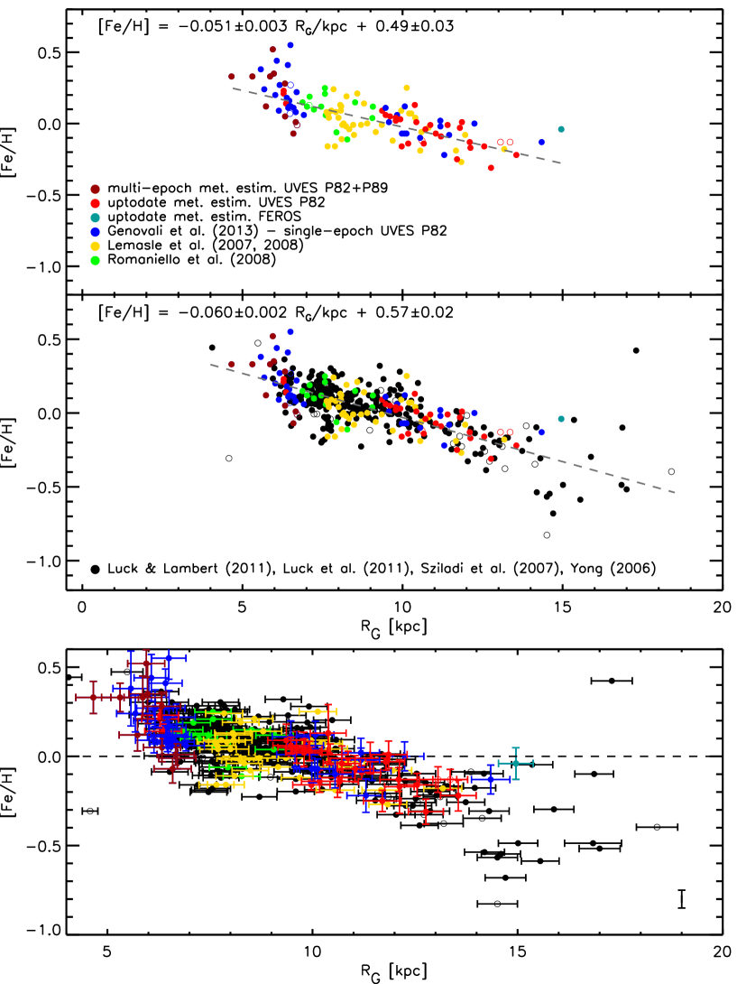
Figure 4: Top – Iron abundances of Galactic classical Cepheids versus Galactocentric distance. Spectroscopic measurements based on different data sets are plotted with different colors. They include updated iron abundances based on current UVES spectra (30, red) and on multi-epoch UVES spectra (11, dark red); plus updated iron abundance for CE Pup based on a FEROS spectrum (light blue) and iron abundances provided by our group: Genovali et al. (2013) (33, blue), Lemasle et al. (2007), Lemasle et al. (2008) (39, yellow), Romaniello et al. (2008) (14, green). Cepheids that according to the General Catalog of Variable Stars (Samus et al., 2009) are candidate classical Cepheids were plotted with open circles. The grey dashed line shows the metallicity gradient. Middle – Same as the top, but the iron abundances include our measurements and those available in the literature: Luck et al. (2011), Luck & Lambert (2011), and Sziládi et al. (2007) (322, black). The grey dashed line shows the metallicity gradient based on the entire sample. Bottom – Zoom of the top panel for Galactocentric distances ranging from 4 to 20 kpc. The bars on individual Cepheids display the uncertainty both on iron abundance and on distance. The vertical black bar on the bottom right corner shows the mean uncertainty on Luck & Lambert (2011) and Romaniello et al. (2008) iron abundances.

The top panel of Fig. 4 shows the iron abundances based on UVES multi-epoch spectra of the observing run B (eleven, dark red circles), on UVES single-epoch spectra of the observing run A (30, red circles) and on the FEROS spectrum (light blue circles) as a function of the Galactocentric distances ($R\rm_{G}$). The blue circles display the iron abundances provided by Genovali et al. (2013) based on UVES single-epoch spectra of the observing run A (33 stars). Together with the current sample, we also included iron abundances for Galactic Cepheids estimated by our group using the same approach and similar data (Lemasle et al. 2007; Lemasle et al. 2008; 39 objects, green circles; Romaniello et al. 2008; 14 objects, yellow circles). Current data set covers a range in Galactocentric distances of more than 10 kpc (4 $\lesssim R_{G}\lesssim R_{G}$ 15 kpc). We estimated the metallicity gradient (dashed line) and we found [Fe/H]=0.49$\pm$0.03 - 0.051$\pm$0.003 $R_{G}$/kpc. The new slope and zero–point agree quite well with similar estimates available in the literature (Luck & Lambert, 2011; Lemasle et al., 2013). The spread in iron appears to be homogeneous over the entire galactocentric range, but in the innermost disk regions it increases and becomes of the order of 0.5 dex.

We also included Cepheid iron abundances available in the literature:

Yong et al. (2006); Sziládi et al. (2007); Luck & Lambert (2011); Luck et al. (2011) (322 objects, black circles). The priority for objects in common among different data sets was given to the current sample, then to iron abundances obtained by our group and finally to abundances available in the literature.

It is worth mentioning that we have been able, thanks to the current large and homogeneous data set of NIR mean magnitudes, to include in the analysis of the metallicity gradient 18 Cepheids for which the iron abundance was provided by Luck & Lambert (2011), but for which the individual distances were not available. We ended up with a sample of 450 Cepheids with a homogeneous metallicity scale and a homogeneous distance scale.

The metallicity gradient we found is [Fe/H]= 0.57$\pm$0.02 -0.060$\pm$0.002 $R_{G}$/kpc, in very good agreement with previous results from Luck & Lambert (2011) based on a similar number of Cepheids. Note that to identify possible outliers, we performed a preliminary gradient estimate and we found [Fe/H]= 0.54$\pm$0.02 -0.057$\pm$0.002 $R_{G}$/kpc. Subsequently, we neglected four Cepheids –BC Aql, HK Cas, EK Del, GP Per– with a gradient residual greater than 3$\sigma$. Three out of the four neglected Cepheids are classified in the GCVS as candidate Cepheids (CEP), while HK Cas is very high on the Galactic plane and it has been classified as an Anomalous Cepheid by Luck & Lambert (2011).

The new metallicity gradient still shows a large intrinsic dispersion around the Solar Circle and in the outer disk (Fig. 4) with the possible occurrence either of a change in the slope or of a shoulder for $7\leq R\rm_{G}\leq$10 kpc, as suggested by Twarog et al. (1997); Caputo et al. (2001); Andrievsky et al. (2004).

To further constrain the nature of the spread in iron along the metallicity gradient the anonymous referee suggested to check its depdendency on the distance from the Galactic plane. We selected the Cepheids in our sample with a distance above the Galactic plane smaller than 300 pc and we found that the gradient is quite similar: [Fe/H]=0.49$\pm$0.03 - 0.052$\pm$0.004 $R_{G}$/kpc. We performed the same test by using the entire sample and the gradient is once again minimally affected, and indeed we found [Fe/H]= 0.53$\pm$0.02 -0.055$\pm$0.002 $R_{G}$/kpc. The subsample located closer to the Galactic plane was also adopted to constrain the spread in iron of the outer disk ($R_{G}\geq 13$ kpc). We found that the spread decreases from 0.17 dex (30 Cepheids) to 0.13 dex (9 Cepheids). This means that the difference decreases from 13% to 5% higher than the mean spread over the entire disk (0.11 dex).

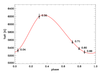
Figure 3: Top – Effective temperature curve versus pulsational phase for the Cepheid RY Sco as derived using the LDRs method (see text for details). The adopted spectra are the same of Fig. 1. The $T\rm_{eff}$ estimates derived for each spectrum and its error, are plotted as black triangles. The red line shows the spline fit. The number plotted on top of the individual measurements show the pulsation phase. Bottom – Same as the top, for the surface gravity.

The referee also noted that the spread in iron abundance around the Solar circle is larger than the spread in the region between 10 and 14 kpc and suggested that the difference might be caused by a different azimuthal distributions of the Cepheids in the two disk regions. To further constrain the dependence of the spread on the azimuthal distribution we estimated, following Genovali et al. (2013), the metallicity distribution of the four Galactic quadrants. We found that the $\sigma$ of the four distributions attain very similar values (0.013$\pm$0.01 dex), while the mean iron abundance increases by almost 0.2 dex when moving from the quadrants I/II to the quadrants III/IV (see Fig. 3 in Genovali et al. 2013). The reader interested in a more quantitative analysis of the variation of the spread along the metallicity gradient is referred to section 6.

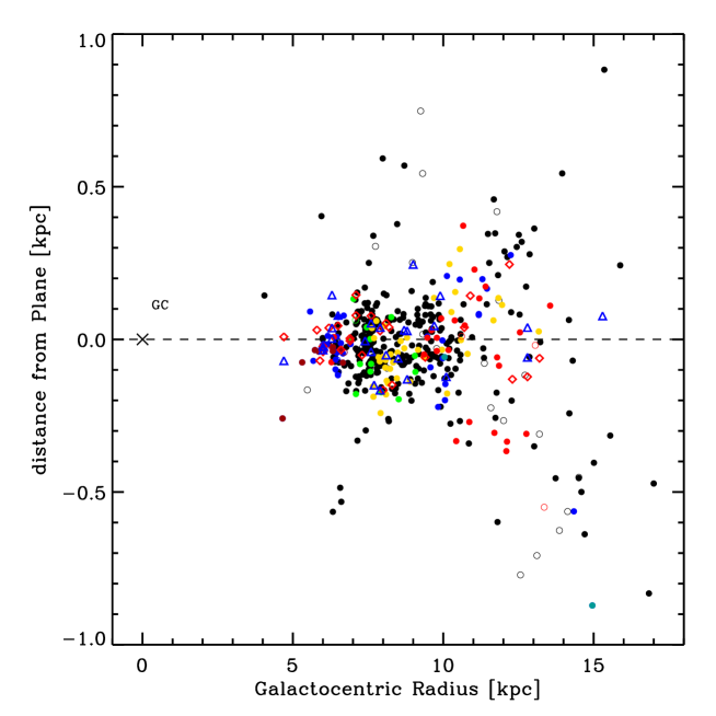
Figure 6: Distance from the Galactic plane versus Galactocentric distance of Galactic Cepheids with accurate iron abundances. Symbols and colors are the same as in Fig. 4 the black cross marks the position of the Galactic Center (GC).

The iron abundances of the current investigation cover the outer disk $R\rm_{G}\geq$ 13 kpc and together with iron abundances provided either by our group or available in the literature do provide a detailed sampling over a broad range of Galactocentric distances ($4\leq R\rm_{G}\leq 19$ kpc). Data plotted in Fig. 4 display a steady increase in the metallicity dispersion when moving from the solar circle to the outer disk. It is interesting to note that Cepheids located in the outer disk also show larger distances from the Galactic plane ($|z|$ $\geq$ 400 pc) when compared with inner disk and solar circle Cepheids (see Fig. 6). However, we did not find a clear correlation between distance from the Galactic plane and metallicity. To constrain on a more quantitative basis the above difference, we analyzed the Cepheid azimuthal distribution and we found, as expected (Kraft & Schmidt, 1963), that they are on average $\sim$38$\pm$13 pc below the Galactic plane and their $\sigma$ is $\sim$270 pc. However, the fraction of Cepheids located at distances from the Galactic plane larger than 1$\sigma$ increases from 4% for $R\rm_{G}$ smaller than 10 kpc to 38% at larger Galactocentric distances.

It is worth mentioning that the evidence of an increase in the dispersion of the iron abundance in the outer disk is further supported by the fact that the use of homogeneous iron abundances has further decreased the intrinsic spread from 0.12 (see Fig. 2 of Genovali et al. 2013) to 0.10 dex (see Fig. 4) for $R\rm_{G}$ $\sim$ 11 -15 kpc.

5 Comparison between Cepheid and independent metallicity gradients

5.1 Young tracers

During the last few years several investigations have addressed the open problem concerning the age dependence of the metallicity gradient. This issue has been investigated not only from the empirical (see, e.g., Maciel et al., 2003; Nordström et al., 2004; Henry et al., 2010; Yong et al., 2012) but also from the theoretical point of view. In particular, it has been discussed the role that different stellar tracers can play in constraining the chemical tagging not only in spatial distribution but also in time (Freeman & Bland-Hawthorn 2002).

To further constrain the age effect on the metallicity gradient we collected several abundance gradients based on different stellar tracers.

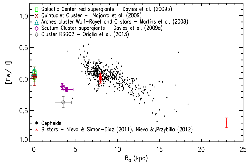
Figure 5: Comparison of the Cepheid (black dots) metallicity gradient with iron abundances of early B–type stars located either in the solar neighborhood or in the Orion star forming region (Nieva & Simón-Díaz, 2011; Nieva & Przybilla, 2012). The green square marks the iron abundance of the two red supergiants in the Galactic center measured by (Davies et al., 2009a), while the magenta diamonds the 26 red supergiants in the Scutum Clusters measured by (Davies et al., 2009b), the grey diamond the three red supergiants in the cluster RSGC2 measured by (Origlia et al., 2013), the red cross the two luminous blue variables (LBVs) in the Quintuplet cluster (Najarro et al., 2009) and the light-blue triangle three Wolf–Rayet and two O-type stars in the Arches cluster (Martins et al., 2008). The red vertical bar on the bottom right corner shows the mean uncertainty on iron abundances.

Fig. 5 shows the comparison between the metallicity gradient based on Cepheids with the iron abundance of almost three dozen of early B–type stars (red triangles) located either in the solar neighborhood (Nieva & Przybilla, 2012) or in the nearby Orion star forming region (Nieva & Simón-Díaz, 2011). The key advantage of this set of measurements is that they are based on high–resolution, high signal–to–noise spectra, they are homogenous and they also account for non=LTE effects (Przybilla et al., 2011).

The comparison of the iron abundances is further supporting the evidence that early B–type stars and classical Cepheids display similar abundance in the solar neighborhood. The spread in iron of the B–type stars is smaller (see the red vertical error bar plotted in the right corner) compared with the Cepheids, but they also cover a narrow disk region. Note that the comparison appears even more compelling if we account that B–type stars are the typical progenitors of classical Cepheids.

The above scenario concerning the iron abundance gradient of young stellar tracers shows a stark difference when compared with iron abundances of young stars (red supergiants, luminous blue variables, Wolf–Rayet and O-type stars) located either in the Nuclear Bulge or in the near end of the Galactic Bar (Martins et al., 2008; Davies et al., 2009a, b; Najarro et al., 2009). Indeed, the above spectroscopic measurements suggest either a solar or a subsolar iron abundance. This finding has been soundly confirmed by Origlia et al. (2013) by using high-spectral resolution ($R\sim$50,000) NIR spectra collected with GIANO at TNG. They found that the mean iron abundance of three RSGs located in the RSGC2 cluster are sub-solar. This finding does not seem to be supported by recent chemical evolution models by Minchev et al. (2013), since they predict in the innermost Galactic regions present days super-solar iron abundances.

The open clusters (OCs) have several advantages as stellar tracers of the Galactic thin disk. i) They typically host a sizeable sample of RGs, this means that multi-object spectrograph can provide very accurate measurements for both iron and $\alpha$-elements. ii) Their distances can be evaluated with good precision by using the main sequence fitting. iii) They trace a significant fraction of the Galactic disk (see the WEBDA website) and their ages range from several hundred of Myrs to several Gyrs. The main drawback is that they are affected by high reddening and quite often by differential reddening. To fully exploit the advantages in using OCs to constrain the metallicity gradient, we selected a sample of 67 OCs for which are available in the literature spectroscopic measurements of iron abundances. To provide a homogeneous metallicity scale for OCs, the individual estimates were rescaled to the solar iron abundance we adopted in this investigation. For the OCs with multiple estimates of the iron abundance in the literature, we typically adopted the most recent measurement. The columns 4 and 5 of Table LABEL:tab:OCs give both the original and the rescaled iron abundance, while columns 6 and 7 give the reference for the metallicity and for the age/distance.

In dealing with Galactocentric distances of OCs, the main source of uncertainty is the calibration of the adopted distance indicator.

Moreover and even more importantly, age estimates are tightly correlated with the adopted cluster distance, reddening and metallicity. The cluster age also depends on the evolutionary framework (overshooting, mass loss, rotation, microphysics) adopted to compute evolutionary models and cluster isochrones (Bono et al., 2001e; Salaris & Cassisi, 2008; Prada Moroni et al., 2012; Neilson et al., 2012b; Anderson et al., 2013). To overcome this thorny problem and to limit their intrinsic dispersion in the metallicity gradient we decided to only use OC with homogeneous estimates of the four crcuail parameters: age, distance, reddening, abundance, theoretical framework. In particular, we selected determinations provided by Salaris et al. (2004) and Friel (1995) (30 OCs), by the Carraro’s group (13 OCs), by BOCCE (8 OCs), and by Friel & Janes (1993) (8 OCs). We adopted the Yong et al. (2012) values for 2 remaining OCs. For seven OCs selected by Cheng et al. (2012) we adopted the parameters given by WEBDA and for PWM4 the estimates provided by Yong et al. (2012). The Galactocentric distances are listed in column 3 of Table LABEL:tab:OCs and they were calculated by using the same value of the Sun Galactocentric distance ($R\rm_{G}=7.94$ kpc).

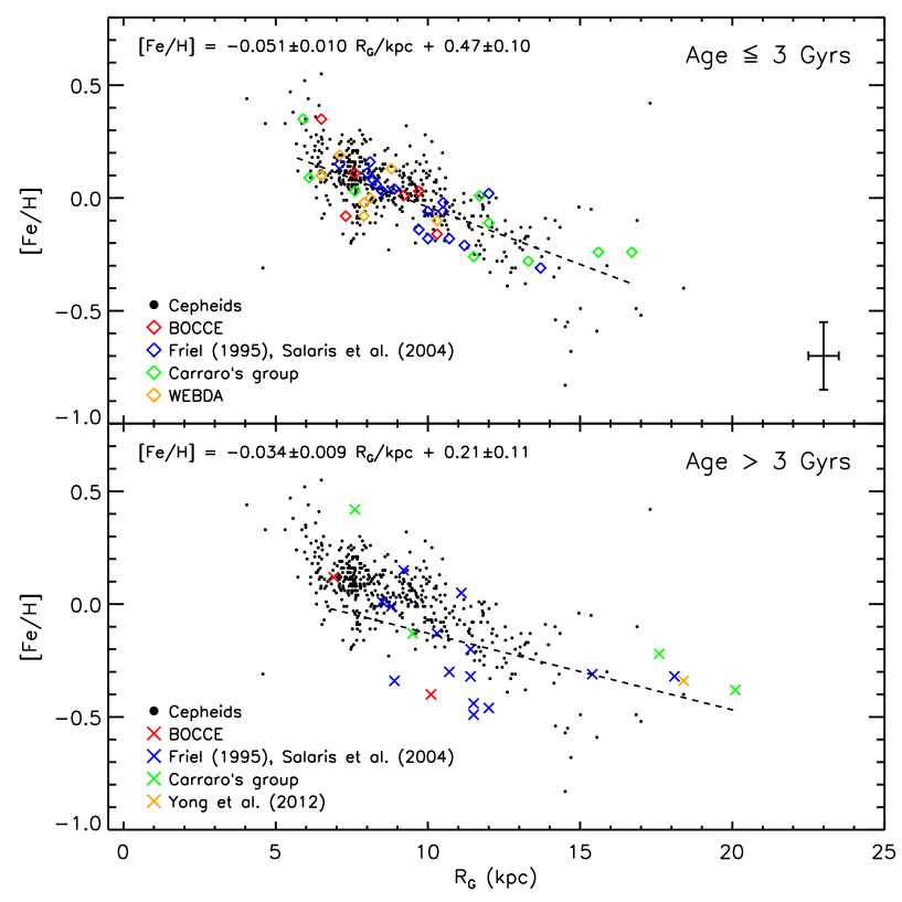
Figure 7: Top – Comparison of the Cepheid (black dots) metallicity gradient with iron abundances for open clusters younger than 3 Gyrs. The color coding does refer to different subsamples: BOCCE project (red symbols); cluster ages from Salaris et al. (2004) and distances from Friel (1995) (blue); Carraro et al. (green symbols); WEBDA (yellow symbols). See Table LABEL:tab:OCs for individual values and references. The vertical and horizontal black error bars on the bottom right corner show the mean uncertainty on Galactocentric distances and iron abundances for OCs in the above subsamples. The dashed line shows the metallicity gradient based on the selected open clusters. Bottom – Same as the top, but for cluster ages older than 3 Gyrs. The yellow cross marks the position of the subsample from Yong et al. (2012). The dashed line shows the metallicity gradient based on the selected open clusters.

The top panel of Fig. 7 shows the comparison between Cepheids (black dots) and 44 OCs younger than 3 Gyrs. Diamonds display the position of OCs and different data sets are marked with different colors (see also Table LABEL:tab:OCs). Data plotted in this panel show that Cepheids and OCs younger than 3 Gyrs are characterized by similar trends when moving from the inner to the outer disk. The same outcome applies, within the errors, to the intrinsic dispersion.

We found a metallicity gradient for the young OCs in our sample of [Fe/H]= 0.47$\pm$0.10 - 0.051$\pm$0.010 $R_{G}$/kpc (see the top panel of Fig. 5), in which both the slope and the zero–point attain values very similar to the Cepheid metallicity gradient (see Fig. 4).

5.2 Intermediate–age tracers

The bottom panel of Fig. 7 shows the same comparison as the top panel, but for OCs (23) with ages ranging from 3.6 to 9 Gyrs. Data plotted in this panel show two distinctive features. i) Old OCs display a clear flattening in iron abundance for $R_{G}\geq 15$ kpc. ii) The old OCs for Galactocentric distances between the solar circle and 12 kpc seem to show a dichotomic distribution. The difference is of the order of several tenths of dex, i.e. larger than possible uncertainties affecting individual iron abundances. We also checked the position of the seven OCs that are, at fixed Galactocentric distance more metal-poor and we found that five out of the seven cover a very narrow range in Galactic latitude (y$\sim$3.5 kpc). Data plotted in the above figure support the evidence that the metallicity gradient depends on age for ages older than $\sim$3 Gyrs. We could also speculate that there is a dozen of OCs distributed along a metal–poor plateau with an almost constant iron abundance ([Fe/H]$\sim$-0.4) and Galactocentric distances ranging from 9 to 21 kpc.

We estimated the metallicity gradient of the older OCs and we found of [Fe/H]=0.21$\pm$0.11 - 0.034$\pm$0.009 $R_{G}$/kpc (see the bottom panel of Fig. 5). The slope and the zero–point are significantly shallower than for Cepheids and younger open clusters and agree quite well similar estimates avaialble in the literature for old OCs (Carraro et al., 2007b; Yong et al., 2012). However, our sample of OCs covers a range in age of five Gyrs and the sample is modest. More solid constraints call for larger samples of OCs and a wider disk coverage.

However, data plotted in the bottom panel of Fig. 7 show that the Cepheid iron abundances in the inner disc are more metal–rich than thin disk old OCs. Moreover, the Cepheids display a well-defined iron gradient when moving from the inner to the outer disc (5 $\leq R_{G}\leq 18$ kpc). However, the above evidence relies on stellar populations with significantly different ages. The Cepheids and the supergiants of the Nuclear Bulge and of the Bar have ages ranging from a few Myrs to a few hundreds of Myrs.

The above findings indicate that younger tracers appear to be still in situ, i.e. in the same regions where they formed, while the intermediate-age tracers appear to be affected both by radial gas flows and by radial migration, as suggested by chemical evolution models (Portinari & Chiosi, 2000; Curir et al., 2012; Minchev et al., 2013). However, current data do not allow us to constrain the timescale within whom the metallicity gradient becomes shallower.

6 The fine structure of the metallicity gradient

We are facing the evidence that the intrinsic dispersion of the iron metallicity gradient is, at fixed Galactocentric distance, systematically larger than the expected standard deviation (see the error bar in the right corner of the bottom panel of Fig. 4). This circumstantial evidence stimulated several investigations aimed at constraining the physical reasons for such a broad distribution. On the basis of a large Cepheid data se,t Luck et al. (2006) suggested that the large dispersion in iron abundance for Galactocentric distances of $R_{G}$ $\sim$ 9-11 kpc was caused by a metallicity island located at $l=130^{\circ}$. However, the detection of well defined region characterized by a higher iron abundance was not supported in a subsequent analysis by Luck & Lambert (2011) by using a larger Cepheid sample. The evidence of a clumpy metallicity distribution across the Galactic disk was also brought forward by Lemasle et al. (2008) and by Pedicelli et al. (2009) by using similar samples of Galactic Cepheids. However, the evidence was partially hampered by the sample size and by the lack of a homogeneous metallicity scale.

6.1 Identification of Cepheid Groups

To further constrain the above preliminary evidence we decided to follow a different approach. We performed a new search for Cepheids Groups (CGs) across the Galactic disk. The search in 3D space follows a method originally suggested by Battinelli (1991) and applied to Galactic Cepheids by Ivanov (2008, hereinafter I08). He adopted $J$,$H$,$K$ 2MASS photometry for 345 Galactic Cepheids and identified 18 CGs. Current approach when compared with I08 has several advantages: i) we are dealing with a Cepheid sample that is 30% larger and they cover more than 15 kpc across the disk; ii) individual Cepheid distances are independent of reddening corrections; iii) the 56% of NIR Cepheid mean magnitudes are based on multi-epoch light curves.

We ranked the entire Cepheid sample and arbitrarily selected the first one as a pivot and estimated its closest neighbourhood by using their rectangular coordinates x,y and z. Then, we selected the second Cepheid as a pivot, but we removed from the list the first one. In the next step, we selected the third Cepheid in our list as a pivot, but we removed from the list the first and the second one. This process is iterated until we rich the last but one Cepheid in our list. Thus we are left with a set of N-1 pair distances that provide, by definition, a path connecting the entire Cepheid sample, the so called ”Path Linkage Criterion” (Battinelli, 1991). The two main positive features of the above algorithm are that a region with a high concentration of short pair distances is also a region in a 3D space with a high concentration of Cepheids. Moreover, the use of relative distances on a common path provides solid detections of filamentary groups (Battinelli, 1996).

Once we have the set of pair distances, we need to define on the basis of our Cepheid sample a characteristic distance called ”search distance” –$d_{S}$– that will allow us to identify candidate Cepheid groups. In particular, we define a candidate Cepheid group if $m$ Cepheids (with $m\geq$6) have a distance $d<d_{S}$, where $d_{S}$ is an arbitrary distance in kpc. We adopted $d_{S}$ distances ranging from 0.1 to 0.8 kpc with a step in distance of 0.05 kpc. Fig. 8 shows the number of independent CGs we detected as a function of the searching distance. The distribution of candidate CGs we found is similar to the distribution found by I08. However, the current peak of the distribution is slightly smaller (13 vs 18) and takes place at smaller $d_{S}$ distances (0.25 vs 0.40 kpc). Moreover, the number of candidate CGs decreases quite rapidly for $d_{S}$ distances larger than $\sim$0.6 kpc while I08 detected CGs at $d_{S}$ distances larger than 1 kpc (see Fig. 3 in I08). The difference might be explained with the difference in sample size and in the adopted Cepheid distances.

Once we have defined the optimal search distance for our Cepheid sample we need to define a criterion to constrain how significant is the density of the individual candidate CG when compared with the average stellar density of its neighbourhood. In particular, we define a bonafide CG only the candidate CGs whose density –$\rho_{CG}$– is four times larger than the density of a spherical layer –$\rho_{sl}$– centered on the center of mass of the CG. The outer radius of the spherical layer –$R_{sl}$– was fixed in such a way that the volume of the spherical layer is three times larger than the volume of the CG. In particular, $V_{sl}$=3$V_{CG}$= $4\pi(R_{sl}-R_{CG})^{3}$/3 where $V_{CG}$ is the volume of the candidate CGs estimated by using a Montecarlo method an by assuming for each Cepheid in the group a radius equal to the adopted search distance ($d_{S}$). The radius of the candidate CG was defined as $R_{CG}$=1.1$\times$ $\delta$, where $\delta$ is the distance of the two most distant Cepheids. Note that $R_{CG}$ is also by construction the inner radius of the spherical layer adopted to estimate the difference in density between the candidate CG and its stellar neighbourhood.

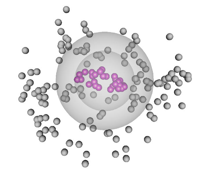
Figure 9: 3D plot showing the approach we adopt to select candidate CGs. The members of a generic CG are displayed with magenta sphere, while the surrounding Cepheids with grey spheres. The dark grey shaded inner area shows the sphere including the members of the CG (the radius $R_{CG}$). The light grey shaded outer area shows the spherical layer with a volume three times larger than the volume of the selected CG. Candidate CGs have a Cepheid density that is 3.5 larger than the average stellar density of its neighborhood.

Fig. 9 shows a 3D graphical view of the approach we adopted to estimate the density of the candidate CGs and the density of the spherical layer. The members of the candidate Cepheid group are plotted as magenta spheres, while the inner light grey sphere defines $V_{CG}$, i.e. the volume of the sphere (with radius equal to $R_{CG}$) adopted to estimate the density of the candidate CG ($\rho_{CG}$). The dark grey sphere defines $V_{sl}$, i.e. the volume of the spherical layer of outer radius $R_{sl}$ and inner radius $R_{CG}$ adopted to estimate the average density of the stellar vicinity ($\rho_{rl}$).

In order to fix the cutoff density for the identification of CGs, we performed a series of numerical experiments in which we randomly distributed the same number of Cepheids across the Galactic disk and we found that their densities are systematically smaller than four times the densities of the spherical layers. By adopting this conservative selection criterion we ended up with ten candidate CGs. The overdensities of the selected CGs range from 4.1 to 45.7 when compared with their stellar neighborhood. The coordinates and the Galactocentric distances of the newly identified Cepheids are listed in columns 1 to 5 of Table 6 together with their diameters and the number of members. The smaller groups have on average 6–7 members and have sizes of the order of half a kpc, while the largest ones have 20–50 members and sizes between 1.2 and 1.9 kpc. The above dimensions are similar to the typical size of giant molecular clouds (see Fig. 3 in Bolatto et al. 2008 and Table 1 in Murray 2011) and to the typical size of giant star complexes and superassociations (Elmegreen & Elmegreen, 1983; Efremov, 1995).

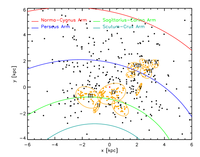
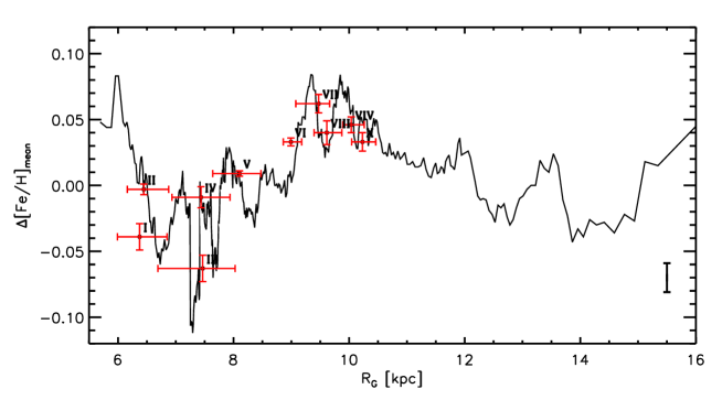
Figure 10: Top – Projection onto the Galactic plane of isolated Cepheids (black dots) and Cepheids members of candidate CGs (yellow dots). The ellipses mark the edges of individual CGs. They are also labeled with the identification number given in Table 6. The red dot shows the Sun position. The colored lines display a logarithmic model of the spiral arms (Vallée, 2002; Cordes & Lazio, 2002, see text for details). The names of the spiral arms are labeled. Bottom – Running average of Cepheids metallicity residuals versus Galactocentric radius (black line). The red dots mark the mean metallicity of the candidate CGs once the metallicity gradient has been subtracted. The red vertical lines display the intrinsic dispersion in iron of candidate CGs. The red horizontal lines show the inner and the outer Galactocentric distance of individual candidate CGs (see columns 6 and 7 in Table 6).

To further constrain the spatial distribution of the newly identified candidate CGs, the top panel of Fig. 10 shows their projection (filled circles) onto the Galactic plane. The members of the individual candidate CGs are plotted in yellow and confined by ellipses. Each group is marked by an increasing Roman number according to the Galactocentric radius. In order to find a correlation between the location of candidate CGs and the spiral arms, we also plotted a simplified model of the disk spiral structure. We used the logarithmic model presented by Vallée (2002) with four arms and a pitch angle of 12 degrees. The logarithmic parameter $r_{0}$ = 2.58 was fixed in such a way that the Perseus arm overlaps with the fiducial points of the model provided by Cordes & Lazio (2002). We adopted this empirical calibration because Xu et al. (2013) found that the latter disk model fits quite well the parallax data of 30 masers associated with star-forming regions in the Perseus and in Sagittarius arms.

The true location of the spiral arms is not well defined, since it depends on the adopted tracers whose distance is quite often poorly known. However, data plotted in the top panel of Fig. 10 indicate a correlation between candidate Cepheid groups and star formation regions associated with the spiral arms.

6.2 Residuals of the metallicity gradient

To further investigate the physical connection of the individual members of the candidate CGs, we analyzed the residuals of the metallicity gradient. We estimated for each Cepheid in our sample the difference between its iron abundance and the iron abundance of the metallicity gradient at the same Galactocentric distance. To avoid spurious fluctuations in the mean iron abundance, we ranked all the Cepheids as a function of the Galactocentric distance ($R_{G}$) and estimated the running average by using the first 20 objects in the list. The mean $R_{G}$ and the mean residual ($\Delta[Fe/H]$) of the bin were estimated as the mean over the individual Galactocentric distances and residual abundances of the same 20 objects. We estimated the same quantities by moving one object in the ranked list until we accounted for the last 20 Cepheids in the sample with the largest distances. The running average is plotted as a black line in the bottom panel of Fig. 10. The error on the mean residual for individual bins is of the order of a few hundredths of dex. In order to provide robust constraints on the possible uncertainties introduced by the adopted number of Cepheids per bin and by the number of stepping stars, we performed a series of Monte Carlo simulations. The estimated mean dispersion of the above simulations is plotted as a vertical black line.

Interestingly enough, the residuals display local minima and maxima that are significantly larger than the intrinsic dispersion. The occurrence of the above chemical inhomogeneities is well defined for Galactocentric distances smaller than 11 kpc. Unfortunately, the current sample does not allow us to rich firm conclusions concerning the outer disk. To constrain the nature of the secondary features in the residuals, we overplotted in the bottom panel of Fig. 10 the position of the ten candidate CGs (red dots). We adopted the mean Galactocentric distance and the mean iron abundance of the individual CGs listed in columns 5 and 14 of Table 6 and subtracted the iron abundance of the metallicity gradient at the same $R_{G}$. The red vertical lines display the standard deviation of the iron abundances, while the horizontal red lines display the inner and the outer edge of the individual CGs (columns 6 and 7 of Table 6).

Data plotted in this figure show that the residuals in iron abundance appear to be tightly correlated with the mean residual abundance abundance of the candidate CGs. This finding further supports the evidence that a significant fraction of the intrinsic dispersion of the metallicity gradient is caused by the presence of Cepheid Groups across the Galactic disk with mean metallicities that are either more metal–rich or more metal–poor than expected according to a linear mean metallicity gradient. The mean periods and their intrinsic dispersions listed in columns 10 and 11 of Table 6 seem to suggest that the candidate CGs with negative iron residuals have on average slightly longer periods and larger intrinsic dispersions when compared with the candidate CGs showing a positive iron residual. However, this evidence could be caused by an observational bias, and indeed the former candidate CGs have higher Cepheid densities (see columns 9 and 13 of Table 6) when compared with the latter ones. The pulsation and evolutionary properties of the candidate CGs will be discussed in a forthcoming paper.

The above empirical evidence have also implications concerning the chemical enrichment of the Galactic disk. During the last few years it has been suggested that iron and oxygen abundances do show a break in the abundance gradient associated with the corotation resonance of the spiral pattern (see e.g. Acharova et al., 2010). This evidence applies not only to external spiral galaxies (Scarano et al., 2011; Scarano & Lépine, 2013), but also to our Galaxy (Lépine et al., 2011). In particular, it has been suggested that the breaks in iron, $\alpha$-elements and barium abundance gradients of Cepheid and open cluster are caused by the corotation resonance located at $R_{G}\sim$9.0–9.5 kpc (Lépine et al., 2013). The occurrence of a discontinuity at the above Galactocentric distance is further supported by the presence of a well defined local minimum in the Galactic rotation curve (see Figures 1, 3 and 5 in Sofue et al. 2009). On the basis of the above preliminary evidence it has been suggested that the Galaxy is experiencing a bimodal chemical evolution, since the kinematic of the gas has opposite directions at the corotation resonance of the spiral pattern.

However, current iron abundances for Galactic Cepheids do not show either a break or a jump or a change in the slope for $R_{G}\sim$9.0–9.5 kpc. Moreover and even more importantly, the positive iron residual located at the above Galactocentric distance appears to be associated with the five candidate CGs that are located across the Perseus arm (see the solid blue line in the top panel of Fig. 10). Note that the association between the candidate CGs and the Perseus arm does requires a more detailed analysis, since we adopted a qualitative model of the Galactic logarithmic spiral arms (Vallée, 2005). In passing we note that current finding, once confirmed by independent stellar tracers, supports the suggestion brought forward by Sofue et al. (2009) and by Sofue (2013) that the dip in the rotation curve $R_{G}\sim$9.0–9.5 is caused by a massive ring associated with the Perseus arm.

7 Luminosity amplitudes and metallicity dependence

During the last few years the dependence of the luminosity amplitude on metallicity has been investigated both from the theoretical (Bono et al., 2000b) and the observational (Klagyivik & Szabados, 2009; Pedicelli et al., 2010; Klagyivik et al., 2013) point of view. In particular, Szabados & Klagyivik (2012), by using a large sample (327) of Galactic Cepheids with accurate pulsation parameters and spectroscopic metal abundances, found evidence that the luminosity and the radial velocity amplitudes slightly decreases with increasing iron abundance. However, no firm conclusion has been reached, since Pedicelli et al. (2010) by using a similar data set did not find a clear dependence on metallicity. More recently, Klagyivik et al. (2013) by using short–period ($\log P\leq 1.02$) Cepheids found that the $R_{21}$ and the $R_{31}$ Fourier amplitude ratios decrease for increasing iron abundance.

To further constrain the behavior of this interesting diagnostic we took advantage of the current sample of Galactic Cepheids with homogeneous spectroscopic abundances. We limited our sample to fundamental Cepheids for which are available accurate V-band amplitudes and we ended up with a sample of 351 Cepheids. However, the period distribution of Galactic Cepheids shows a short tail in the long–period range when compared with Magellanic Cloud (MC) Cepheids (Gascoigne, 1974; Bono et al., 2010; Inno et al., 2013; Genovali et al., 2013). To overcome possible biases in constraining the metallicity dependence we took advantage of the MC Cepheids for which were available spectroscopic iron abundances (Luck & Lambert, 1992; Luck et al., 1998; Romaniello et al., 2008) and V-band amplitudes (SMC and LMC field Cepheids: OGLE III [Soszynski et al. (2008), Soszyñski et al. (2010)]; ASAS [Karczmarek et al. (2011), Karczmarek et al. (2012)]; plus data provided by van Genderen (1983), Freedman et al. (1985), Caldwell et al. (1986), van Genderen & Nitihardjo (1989), Caldwell et al. (2001). For cluster Cepheids we adopted data provided by Sebo & Wood (1995) [NGC 1850] and by Welch et al. (1991); Welch & Stetson (1993) [NGC 1866]).

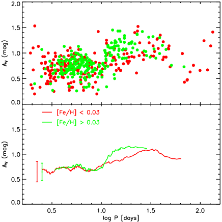
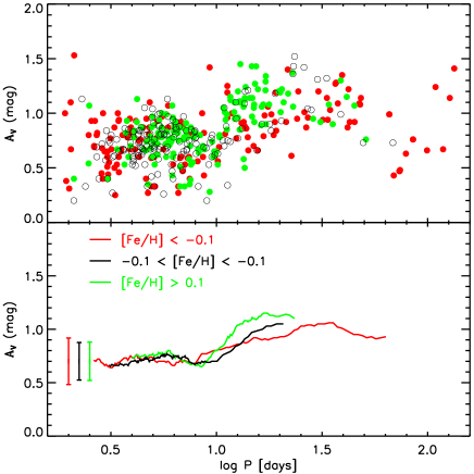
Figure 11: Visual amplitudes versus logarithmic period for Galactic and Magellanic Cepheids. Different colors indicate different metallicity ranges. Top left – the Cepheid sample was divided into two sub-samples: super-solar (green circles) and sub-solar (red) metallicity. Bottom left – Running mean of the luminosity amplitudes plotted in the top panel. The color coding is the same of the top panel. The vertical bars display the intrinsic error of the running mean due to bin size and number of stepping stars (see text for more details). Top right – Same as the top left panel, but the Cepheid sample was divided into three subsamples: super-solar (green), solar (empty black circles), and sub-solar (red) metallicity. Bottom right – Same as the bottom left panel, but for the three different metallicity bins adopted in the top panel.

We ended up with a sample of 58 Large Magellanic Cloud (LMC) and 19 Small Magellanic Cloud (LMC) Cepheids. Note that in the first sample are also included 19 Cepheids belonging to the cluster NGC 1866 and 7 Cepheids belonging to the cluster NGC 1850. The metallicities and the pulsation parameters for the Magellanic Cepheids are listed in Table LABEL:tab:amp. The top left panel of Fig. 11 shows the Bailey diagram (V-band luminosity amplitude vs logarithmic period) for the entire sample (428 stars). The center of the Hertzsprung progression at $\log P\leq$ 1.02 is quite evident. The reader interested in a more detailed discussion concerning the nature of the Hertzsprung progression and its metallicity dependence is refereed to Bono et al. (2000a); Bono et al. (2000b).

In order to constrain the dependence of the luminosity amplitude on the metallicity we split the entire sample into metal-poor ([Fe/H]$\leq$0.03, red circles) and metal-rich ([Fe/H]$>$0.03, green circles). To avoid spurious fluctuations in the mean $A_{V}$ amplitude, we ranked all the Cepheids as a function of the logarithmic period and estimated the running average by using the first 25 objects in the list. The mean $\log P$ and the mean $A_{V}$ of the bin were estimated as the mean over the individual periods and amplitudes of the same 25 objects. We estimated the same quantities by moving one object in the ranked list until we accounted for the 25 Cepheids with the longest periods. The running averages for the metal-poor and the metal-rich samples are plotted as red and green lines in the bottom left panel of Fig. 11. The error on the mean $A_{V}$ for individual bins is of the order of a few hundredths of mag. In order to provide robust constraints on the possible uncertainties introduced by the adopted number of Cepheids per bin and by the number of stepping stars, we performed a series of Monte Carlo simulations. The estimated mean dispersions of the above simulations are plotted as vertical green and red lines. We also found that we can exclude a metallicity dependence of the two subsamples at the 98% confidence level. The two running averages plotted in the bottom panel display a strong similarity in the short–period ($\log P\leq$ 1.02) range, but the difference increases at longer periods. We performed the same analysis by splitting the sample in short- and long–period Cepheids and we found that the metallicity dependence in the former group can be excluded at the 94% level, while the in the latter one at the 70% level.

To further constrain the dependence of the V-band amplitude on metallicity, we performed the same analysis but the entire sample was split into: metal–poor ([Fe/H]$\leq-0.01$), metal–intermediate ($-0.01\leq$ [Fe/H] $\leq+0.01$) and metal–rich ([Fe/H]$\geq+0.01$). The three different subsamples are plotted as red, black and green circles in the top right panel of Fig. 11, while the three running averages and their mean dispersions are plotted in the bottom right panel of the same figure. The outcome concerning the metallicity dependence is quite similar to the above analysis. We found that the metallicity dependence between the metal-poor and the metal-intermediate subsamples can be excluded at the 90% confidence level, while the dependence between the metal-poor and the metal-rich subsample at the 80% level. We also split the sample in short– and long–period and we found that the dependence can be excluded at the 93% and at the 90% level between metal–poor and metal–intermediate Cepheids and at the 90% and at the 77% level between metal–poor and metal–rich Cepheids.

The above findings indicate that the luminosity amplitude of Galactic and MC Cepheids does not display a solid trend with metal abundance. However, current analysis should be cautiously treated for two different reasons: i) The Galactic sample is still dominated by Cepheids at solar iron abundance, since the sample of more metal-poor Cepheids located in the outer disk ($R_{G}\geq$ kpc) is quite limited; ii) The spectroscopic abundances for MC Cepheids are dominated by brighter (long–period) Cepheids. Firm conclusions concerning the metallicity dependence do require larger samples of spectroscopic abundances to further constrain the difference in pulsation amplitude and in period distribution.

8 Discussion and conclusions

We performed accurate new measurements of iron abundances for 42 Galactic Cepheids using high-resolution, high-$S/N$ UVES, NARVAL and FEROS spectra. The iron abundance, for eleven Cepheids located in the inner disk, is based on multi-epoch spectra (from four to six) and their intrinsic uncertainty is smaller when compared with other Cepheids at super-solar iron content. Current sample was complemented with Cepheid iron abundances based on high–resolution spectra provided either by our group (Lemasle et al., 2007; Lemasle et al., 2008; Romaniello et al., 2008; Genovali et al., 2013) or available in literature (Luck et al., 2011; Luck & Lambert, 2011). We ended up with a sample of 450 Cepheids. To improve the accuracy on the metallicity distribution across the disk, we estimated homogeneous and reddening-free distances by using near-infrared Period–Wesenheit relations for the entire sample.

The main findings of the current iron abundance analysis are given in more detail in the following.

• We found that the metallicity gradient, based on current spectroscopic measurements, is linear with a slope of -0.051$\pm$0.003 dex/kpc, in agreement with recent studies by Luck et al. (2011) and Luck & Lambert (2011). The metallicity gradient based both on our and on literature iron abundances shows a similar slope: -0.060 $\pm$ 0.002 dex/kpc. Current estimates agrees quite well with the chemical evolution model for the thin disc recently provided by Minchev et al. (2013). In particular, they found that the iron gradient is -0.061 dex/kpc for Galactocentric distances ranging from 5 to 12 kpc and -0.057 dex/kpc for Galactocentric distances ranging from 6 to 11 kpc. The predicted slopes become marginally shallower if they account for stellar radial migrations.

• We estimated the metallicity gradient by selecting the Cepheids in our sample with a distance above the Galactic plane smaller than 300 pc and we found that it is, within the errors, quite similar: -0.052$\pm$0.004 dex/kpc. The same outcome applies to the the gradient based on the entire sample, and indeed we found: -0.055$\pm$0.002 dex/kpc. We also found that the spread in iron in the outer disk ($R_{G}\geq 13$ kpc) decreases by more than a factor of two (0.13 vs 0.17 dex) if we adopt the subsample located closer to the Galactic plane.

• We also confirm that classical Cepheids in the inner disk ($R\rm_{G}$ $\sim$5.5–6.0 kpc), just beyond the position of the Galactic Bar corotation resonance (Gerhard et al., 2011), attain super-solar ([Fe/H]$\sim$0.4) iron abundances. This result supports similar findings by G13 and by Andrievsky et al. (2002b); Pedicelli et al. (2010); Luck & Lambert (2011).

  There is preliminary evidence that the iron abundance in the innermost Galactic regions (Nuclear Bulge, Galactic Bar) is more metal–poor than predicted by chemical evolution models (Minchev et al. (2013)). Indeed recent spectroscopic iron abundances of young stars (red supergiants, luminous blue variables, Wolf–Rayet, O-type stars) indicate either solar or sub–solar abundances (Davies et al., 2009a, b; Origlia et al., 2013). On the other hand, chemical evolution models suggest in the same regions iron abundances larger than [Fe/H]$\sim$0.8 (Minchev et al., 2013). The above evidence indicate that objects located inside the corotation resonance of the bar experienced a different chemical enrichment history when compared with Cepheids located just beyond this limit.

• The new homogeneous Cepheid metallicity distribution is characterized by a smaller intrinsic dispersion when compared with similar estimates available in the literature. We found evidence of a steady increase in the abundance dispersion when moving in the outer disk ($R\rm_{G}$ ¿ 14 kpc). Current data do no allow us to constrain whether this effect is the aftermath of outward stellar migrators as recently suggested by Minchev et al. (2012) or the consequence of the infall of the Sagittarius dwarf galaxy producing a flared outer disk as suggested by Purcell et al. (2011).

• To investigate the fine structure of the metallicity in the disk, we searched for Cepheids groups following the approach suggested by Ivanov (2008). We found ten candidate Cepheids Groups, i.e. physical aggregation of stars whose mean residual metallicity agrees quite well with the trend of the metallicity residuals as a function of the Galactocentric distance. The presence of the CGs appears to be the main culprit of the fluctuations in the metallicity residuals and of the azimuthal effects on the radial gradient. This suggests that members of CGs experienced a very similar chemical enrichment history. Most of the CGs are located close to spiral arms (Sagittarius-Carina and Perseus arms) according to a simple logarithmic spiral model provided by Vallée (2005). The above findings indicate that the occurrence of CGs with sizes ranging from OB association/young cluster to star complexes/superassociations appear to be largely responsible for the intrinsic spread of the iron metallicity gradient. Moreover, the association of the metallicity residuals with candidate CGs supports the results by Sofue (2013) concerning the association of a local minimum in the Galactic rotational curve at $R\rm_{G}\sim$=9.5 kpc with the Perseus arm.

• We also found that the mean periods of the Cepheids hosted in candidate CGs with negative iron residuals have, on average, slightly longer periods and larger intrinsic dispersions when compared with the candidate CGs showing a positive iron residual. Thus suggesting a common star formation episode within each candidate CG. The evidence of possible abundance inhomogeneities in the Galactic disk dates back to (Efremov, 1995, and references therein) who suggested that the different star complexes might have different star formation histories and different interactions with the intergalactic medium. It is clear that the abundance information (iron and $\alpha$–elements) will provide a new spin to the analysis of their evolutionary and pulsation properties.

• To constrain the impact of age on iron abundance gradient, we compared the Cepheid iron gradient with those based on OCs. Spectroscopic metallicities and homogeneous distances and age were collected for OCs spanning a large range in age. The OC gradient based on clusters younger than 3 Gyrs agrees quite well with the Cepheid gradient.

• The comparison between Cepheids and OCs older than 3 Gyrs is more complex. Indeed, we found that old OCs display a clear flattening in iron abundance for $R_{G}\geq 15$ kpc. This result supports similar findings available in the literature e.g. Carraro et al. (2007b), Bragaglia et al. (2008), Magrini et al. (2009, 2010), Jacobson et al. (2011a, b), Yong et al. (2012). Moreover, old OCs located between the solar circle and $R\rm_{G}\sim$12 kpc seem to show a dichotomic distribution. The difference is of the order of several tenths of dex and might be due to a selection bias affecting the azimuthal distribution. However, the comparison of Cepheids iron abundances with similar abundances for old OCs further support the evidence that the metallicity gradient does depend on age for ages larger than $\sim$3 Gyrs.

• We investigate the possible occurrence of a metallicity effect on the pulsational amplitude by using a large sample of fundamental Galactic and Magellanic Cepheids (Luck & Lambert, 1992; Luck et al., 1998; Romaniello et al., 2008) with accurate iron abundances. The comparison of low, medium, and high metallicity subsamples indicate that luminosity amplitudes are, within current uncertainties, independent of iron abundance.

Classical Cepheids appear to be solid young stellar tracers to constrain the recent chemical enrichment of the Galactic thin disk. Current sample of Galactic Cepheids is smaller when compared with similar tracers (OB stars, HII regions, red clump stars, open clusters). However, their distances, ages and abundances can be firmly estimated. They are ubiquitous in young star forming regions and the recent identification of classical Cepheids both in the Nuclear Bulge and in the Galactic Bar (Matsunaga et al., 2011b, 2013) will provide the opportunity to use the same stellar tracer to constrain the change in iron abundance across the corotation resonance. This also means the opportunity to constrain whether the high star formation rate of the innermost Galactic regions is driven by a disk instability that is dragging material from the inner disk into these regions (Freeman et al., 2013; Ness et al., 2013a, b).

Classical Cepheids are also excellent tracers to constrain the speed of the spiral arm pattern by fitting a kinematic model to the observed Cepheid kinematics (Fernández et al., 2001; Lépine et al., 2001). The Cepheid kinematics is time consuming, since a proper coverage of the radial velocity curves does require spectroscopic time series data. The use of template radial velocity curves significantly decreases the number of measurements required for an accurate estimate of the center of mass radial velocity (Metzger et al., 1998). However, we still lack accurate radial velocity curve templates covering the entire period range.

Current observational scenario appears to be even more appealing in the outer disk, since we are still facing a ”Cepheid desert” for Galactocentric distances larger than $\sim$18 kpc. New identification and characterization of Cepheids at least in the first and in the second quadrant are urgently needed to properly trace the outskirts of the Galactic disk.

Figure 1: High-resolution (R$\sim$38,000) UVES spectra of solar metallicity Galactic Cepheid RY Sco ([Fe/H] = 0.01 $\pm$ 0.06). From top to bottom the spectra were plotted for increasing pulsational phase. (see the corresponding $T\rm_{eff}$ curve in Fig. 3). The SNR of this sample is around 100 in the spectral range $\lambda$ $\sim$ 5650–7500 Å. The vertical dashed lines display selected Fe I ($\lambda\lambda$5930.17, 5934.66, 5952.73, 5956.7, 5975.35, 5976.78, 5983.69, 5984.79, 5987.05, 5997.78 Å) and Fe II ($\lambda\lambda$5932.06, 5991.37 Å) lines included in our abundance analysis (see Table 1 and Romaniello et al., 2008).

Figure 8: Number of candidate Cepheid groups as a function of the ”search distance”. See text for more details.

Table 1: Intrinsic parameters and abundances for the current sample of Classical Cepheids based on individual spectra.

name	date	MJD	ET	$S/N$	$T\rm_{eff}$	log $g$	$v_{t}$	Fe I	N	Fe II	N	Spect.
			(s)		$K$		(km s-1)
V340 Ara	2012-07-29	56137.137	120	99	5210 $\pm$ 49	0.30	5.0	0.28 $\pm$ 0.27	23	0.27 $\pm$ 0.11	2	UVES
V340 Ara	2008-08-30	54708.065	300	241	5210 $\pm$ 88	0.00	3.0	0.53 $\pm$ 0.15	53	0.53 $\pm$ 0.11	4	UVES
V340 Ara	2008-08-31	54709.079	300	264	5130 $\pm$ 96	0.40	3.0	0.42 $\pm$ 0.22	26	0.65 $\pm$ 0.24	3	UVES
V340 Ara	2012-07-30	56138.094	120	122	5610 $\pm$ 68	0.70	4.4	0.30 $\pm$ 0.20	41	0.33 $\pm$ 0.10	2	UVES
V340 Ara	2012-07-31	56139.185	120	114	6060 $\pm$ 65	0.80	5.2	0.24 $\pm$ 0.13	51	0.22 $\pm$ 0.01	2	UVES
V340 Ara	2012-08-13	56152.054	121	69	4820 $\pm$ 53	1.00	4.4	0.20 $\pm$ 0.23	15	0.30 $\pm$ 0.29	2	UVES
AS Aur	2009-01-14	54845.136	500	94	5800 $\pm$ 86	1.10	2.6	0.01 $\pm$ 0.14	74	-0.01 $\pm$ 0.10	8	UVES
KN Cen	2009-01-31	54862.355	80	153	5130 $\pm$ 68	0.01	3.2	0.36 $\pm$ 0.28	14	0.59 $\pm$ 0.13	3	UVES
MZ Cen	2008-04-28	54584.280	800	217	5520 $\pm$ 55	0.90	3.6	0.27 $\pm$ 0.14	45	0.26 $\pm$ 0.14	4	UVES
OO Cen	2008-04-29	54585.060	1500	288	5950 $\pm$ 65	1.00	3.7	0.19 $\pm$ 0.12	30	0.20 $\pm$ 0.07	4	UVES
TX Cen	2009-01-31	54862.363	200	152	5380 $\pm$ 87	0.60	3.8	0.43 $\pm$ 0.16	78	0.45 $\pm$ 0.20	7	UVES
V339 Cen	2008-04-28	54584.304	60	183	5210 $\pm$ 54	0.40	3.2	0.06 $\pm$ 0.14	39	0.06 $\pm$ 0.03	3	UVES
VW Cen	2009-01-31	54862.359	200	144	5190 $\pm$ 65	0.30	4.4	0.40 $\pm$ 0.10	43	0.44 $\pm$ 0.13	2	UVES
AO CMa	2009-01-08	54839.053	900	120	5855 $\pm$ 57	1.30	2.6	0.00 $\pm$ 0.07	75	0.03 $\pm$ 0.11	5	UVES
RW CMa	2009-01-08	54839.138	500	198	6050 $\pm$ 63	1.20	3.0	-0.07 $\pm$ 0.11	83	-0.06 $\pm$ 0.11	5	UVES
SS CMa	2009-01-08	54839.066	80	93	5700 $\pm$ 54	0.60	2.6	0.06 $\pm$ 0.05	57	0.07 $\pm$ 0.10	5	UVES
TV CMa	2009-01-16	54847.246	200	149	5570 $\pm$ 38	1.10	3.0	0.00 $\pm$ 0.11	89	0.01 $\pm$ 0.09	6	UVES
TV CMa	2007-11-03	54407.238	2700	101	5850 $\pm$ 126	1.4	2.6	0.01 $\pm$ 0.09	128	0.06 $\pm$ 0.19	23	NARVAL
TW CMa	2009-01-08	54839.077	80	63	6135 $\pm$ 109	1.20	2.5	0.04 $\pm$ 0.10	38	0.07 $\pm$ 0.30	4	UVES
AA Gem	2009-01-15	54846.149	80	84	5540 $\pm$ 104	0.60	3.0	-0.08 $\pm$ 0.06	74	-0.08 $\pm$ 0.13	5	UVES
AD Gem	2009-01-15	54846.221	80	109	6200 $\pm$ 122	1.60	2.2	-0.17 $\pm$ 0.14	70	-0.13 $\pm$ 0.07	7	UVES
BB Gem	2009-01-15	54846.187	500	160	7000 $\pm$ 253	1.90	2.8	-0.08 $\pm$ 0.13	70	-0.09 $\pm$ 0.04	9	UVES
BW Gem	2009-01-14	54845.122	900	141	5850 $\pm$ 65	1.60	2.2	-0.22 $\pm$ 0.12	99	-0.21 $\pm$ 0.15	6	UVES
DX Gem	2009-01-15	54846.196	200	121	6200 $\pm$ 92	1.60	2.8	-0.01 $\pm$ 0.11	72	-0.01 $\pm$ 0.15	6	UVES
RZ Gem	2009-01-14	54845.094	200	207	7000 $\pm$ 170	1.60	3.4	-0.13 $\pm$ 0.11	44	-0.16 $\pm$ 0.03	5	UVES
BE Mon	2009-01-15	54846.201	200	136	5770 $\pm$ 58	1.50	2.9	0.05 $\pm$ 0.12	78	0.05 $\pm$ 0.13	5	UVES
CV Mon	2009-01-15	54846.182	200	152	5540 $\pm$ 58	0.60	2.6	0.09 $\pm$ 0.10	52	0.11 $\pm$ 0.21	2	UVES
FT Mon	2009-01-14	54845.104	1000	85	5810 $\pm$ 92	1.20	2.7	-0.13 $\pm$ 0.11	61	-0.14 $\pm$ 0.12	8	UVES
SV Mon	2009-01-14	54845.119	30	143	5090 $\pm$ 58	0.10	2.5	0.10 $\pm$ 0.09	54	0.17 $\pm$ 0.15	8	UVES
TW Mon	2008-11-26	54796.347	1000	144	5990 $\pm$ 105	1.30	2.7	-0.13 $\pm$ 0.08	75	-0.13 $\pm$ 0.16	6	UVES
TX Mon	2008-11-28	54798.345	200	109	6180 $\pm$ 62	1.40	3.2	-0.03 $\pm$ 0.15	76	-0.03 $\pm$ 0.05	4	UVES
TY Mon	2009-01-15	54846.139	500	134	6320 $\pm$ 73	1.50	2.3	0.01 $\pm$ 0.11	85	0.03 $\pm$ 0.12	6	UVES
TZ Mon	2009-01-16	54847.237	200	127	5625 $\pm$ 41	1.20	2.9	-0.02 $\pm$ 0.08	94	-0.01 $\pm$ 0.12	6	UVES
V465 Mon	2009-01-16	54847.241	200	144	6250 $\pm$ 56	1.50	2.8	-0.07 $\pm$ 0.11	107	-0.07 $\pm$ 0.10	6	UVES
V495 Mon	2009-01-15	54846.167	1000	126	5590 $\pm$ 57	1.20	3.0	-0.14 $\pm$ 0.09	73	-0.11 $\pm$ 0.10	4	UVES
V508 Mon	2009-01-16	54847.232	200	135	6140 $\pm$ 95	1.70	2.7	-0.06 $\pm$ 0.15	118	-0.03 $\pm$ 0.13	7	UVES
V510 Mon	2009-01-15	54846.153	1000	125	5505 $\pm$ 52	0.90	3.4	-0.15 $\pm$ 0.11	80	-0.17 $\pm$ 0.08	3	UVES
XX Mon	2008-11-28	54798.335	500	93	5590 $\pm$ 47	1.20	2.8	0.00 $\pm$ 0.09	55	0.02 $\pm$ 0.14	2	UVES
GU Nor	2008-07-20	54667.205	300	258	6240 $\pm$ 43	1.40	3.2	0.08 $\pm$ 0.11	80	0.08 $\pm$ 0.07	7	UVES
IQ Nor	2008-04-28	54584.299	150	265	5950 $\pm$ 87	0.70	4.0	0.19 $\pm$ 0.13	63	0.23 $\pm$ 0.09	7	UVES
QZ Nor	2009-02-01	54863.366	30	100	5740 $\pm$ 46	1.10	2.8	0.18 $\pm$ 0.12	81	0.19 $\pm$ 0.12	3	UVES
QZ Nor	2009-04-02	54923.345	30	100	5790 $\pm$ 53	1.00	2.8	0.20 $\pm$ 0.12	86	0.24 $\pm$ 0.09	2	UVES
RS Nor	2009-02-01	54863.361	200	230	6140 $\pm$ 63	1.20	3.2	0.17 $\pm$ 0.12	82	0.19 $\pm$ 0.12	5	UVES
SY Nor	2008-08-30	54708.061	150	170	5550 $\pm$ 64	0.70	3.7	0.26 $\pm$ 0.14	46	0.28 $\pm$ 0.15	5	UVES
SY Nor	2008-08-31	54709.075	150	205	5675 $\pm$ 55	1.00	3.6	0.20 $\pm$ 0.12	58	0.19 $\pm$ 0.13	4	UVES
TW Nor	2008-07-19	54666.127	800	216	5090 $\pm$ 73	0.30	3.5	0.28 $\pm$ 0.20	69	0.27 $\pm$ 0.12	7	UVES
V340 Nor	2009-02-11	54873.376	30	169	5685 $\pm$ 77	0.60	3.4	0.07 $\pm$ 0.10	47	0.08 $\pm$ 0.11	4	UVES
CS Ori	2009-01-14	54845.085	500	128	6390 $\pm$ 162	1.20	2.0	-0.27 $\pm$ 0.08	68	-0.22 $\pm$ 0.09	6	UVES
GQ Ori	2009-01-14	54845.082	30	100	5050 $\pm$ 104	2.80	1.2	0.19 $\pm$ 0.12	92	0.22 $\pm$ 0.12	14	UVES
RS Ori	2009-01-14	54845.100	30	149	6165 $\pm$ 57	1.00	2.6	0.11 $\pm$ 0.13	71	0.11 $\pm$ 0.12	5	UVES
AQ Pup	2009-01-08	54839.075	30	50	5030 $\pm$ 96	0.10	4.4	-0.07 $\pm$ 0.14	14	0.08 $\pm$ 0.05	2	UVES
BC Pup	2009-01-08	54839.147	2000	81	5705 $\pm$ 121	1.40	3.2	-0.31 $\pm$ 0.09	57	-0.32 $\pm$ 0.11	3	UVES
BM Pup	2009-01-08	54839.086	200	80	5526 $\pm$ 84	0.80	2.7	-0.07 $\pm$ 0.11	61	-0.06 $\pm$ 0.11	7	UVES
BN Pup	2009-01-08	54839.109	80	117	5330 $\pm$ 54	0.50	2.6	0.03 $\pm$ 0.06	69	0.05 $\pm$ 0.13	4	UVES
CE Pup	2010-03-31	55286.057	6300	248	5770 $\pm$ 123	0.50	4.0	-0.04 $\pm$ 0.11	67	-0.03 $\pm$ 0.15	3	FEROS
CK Pup	2009-01-08	54839.113	2000	141	6235 $\pm$ 62	1.20	2.4	-0.15 $\pm$ 0.11	72	-0.14 $\pm$ 0.12	4	UVES
CK Pup	2009-01-08	54839.173	2000	156	6200 $\pm$ 108	0.80	2.3	-0.11 $\pm$ 0.11	78	-0.13 $\pm$ 0.11	11	UVES
HW Pup	2008-11-22	54792.249	900	123	5200 $\pm$ 61	0.40	2.6	-0.24 $\pm$ 0.10	70	-0.16 $\pm$ 0.17	3	UVES
LS Pup	2009-01-08	54839.081	200	97	5235 $\pm$ 115	0.40	3.6	-0.12 $\pm$ 0.11	18	-0.13 $\pm$ 0.00	1	UVES
VW Pup	2009-01-01	54832.331	500	142	5600 $\pm$ 78	1.20	3.1	-0.14 $\pm$ 0.07	50	-0.16 $\pm$ 0.13	4	UVES
VZ Pup	2009-01-08	54839.096	80	123	6480 $\pm$ 65	1.00	3.1	0.01 $\pm$ 0.05	27	-0.05 $\pm$ 0.06	2	UVES
WW Pup	2009-01-08	54839.091	200	119	5500 $\pm$ 104	1.20	3.2	0.13 $\pm$ 0.16	18	0.13 $\pm$ 0.00	1	UVES
WY Pup	2009-01-08	54839.100	200	102	6020 $\pm$ 76	1.60	3.2	-0.10 $\pm$ 0.10	49	-0.09 $\pm$ 0.12	6	UVES
WZ Pup	2009-01-08	54839.104	200	113	5660 $\pm$ 41	1.00	2.7	-0.07 $\pm$ 0.07	72	-0.07 $\pm$ 0.09	7	UVES
X Pup	2009-01-08	54839.070	30	69	5070 $\pm$ 115	0.10	4.8	0.00 $\pm$ 0.09	15	0.09 $\pm$ 0.16	2	UVES
KQ Sco	2012-07-31	56139.021	100	87	5030 $\pm$ 40	0.10	4.8	0.26 $\pm$ 0.15	32	0.00 $\pm$ 0.00	0	UVES
KQ Sco	2009-02-11	54873.379	80	150	4905 $\pm$ 80	0.10	4.6	0.51 $\pm$ 0.08	51	0.63 $\pm$ 0.27	4	UVES
KQ Sco	2012-08-13	56152.097	100	100	4915 $\pm$ 53	0.30	3.6	0.30 $\pm$ 0.21	16	0.35 $\pm$ 0.00	1	UVES
KQ Sco	2012-08-24	56163.004	100	85	4840 $\pm$ 62	0.10	5.2	0.22 $\pm$ 0.27	20	0.63 $\pm$ 0.00	1	UVES
KQ Sco	2012-08-27	56166.004	100	97	4930 $\pm$ 53	0.20	4.8	0.21 $\pm$ 0.28	15	0.39 $\pm$ 0.00	1	UVES
RY Sco	2012-08-01	56140.187	20	116	5545 $\pm$ 40	0.60	3.6	0.02 $\pm$ 0.14	74	0.06 $\pm$ 0.01	2	UVES
RY Sco	2008-05-13	54599.412	20	136	5290 $\pm$ 40	0.40	3.7	0.06 $\pm$ 0.09	34	0.06 $\pm$ 0.02	5	UVES
RY Sco	2012-08-13	56152.143	20	116	6200 $\pm$ 54	0.80	5.2	0.01 $\pm$ 0.15	75	0.01 $\pm$ 0.03	3	UVES
RY Sco	2012-08-23	56162.170	20	108	5380 $\pm$ 38	0.40	3.8	0.00 $\pm$ 0.14	66	-0.03 $\pm$ 0.05	2	UVES
RY Sco	2012-08-28	56167.085	20	111	5330 $\pm$ 31	0.70	4.8	-0.05 $\pm$ 0.12	45	-0.03 $\pm$ 0.11	2	UVES
V470 Sco	2008-08-30	54708.073	800	380	5730 $\pm$ 33	0.80	4.4	0.16 $\pm$ 0.10	66	0.16 $\pm$ 0.08	4	UVES
V500 Sco	2012-08-01	56140.191	46	126	5980 $\pm$ 27	1.10	4.6	-0.09 $\pm$ 0.16	86	0.00 $\pm$ 0.05	3	UVES
V500 Sco	2012-08-13	56152.092	45	99	5330 $\pm$ 26	0.60	3.2	-0.04 $\pm$ 0.12	67	0.10 $\pm$ 0.20	3	UVES
V500 Sco	2012-08-23	56162.998	45	101	5280 $\pm$ 31	0.40	3.8	-0.02 $\pm$ 0.17	53	-0.04 $\pm$ 0.17	3	UVES
V500 Sco	2012-08-28	56167.077	45	152	6020 $\pm$ 35	1.10	4.0	-0.11 $\pm$ 0.16	97	-0.11 $\pm$ 0.08	5	UVES
EV Sct	2008-08-30	54708.086	300	224	6025 $\pm$ 65	1.50	2.5	0.10 $\pm$ 0.15	57	0.09 $\pm$ 0.08	3	UVES
RU Sct	2009-03-16	54906.414	120	205	5190 $\pm$ 35	0.10	2.9	0.15 $\pm$ 0.12	95	0.16 $\pm$ 0.05	7	UVES
RU Sct	2009-04-02	54923.375	80	216	5495 $\pm$ 48	0.30	3.0	0.09 $\pm$ 0.10	45	0.09 $\pm$ 0.09	5	UVES
RU Sct	2007-10-31	54404.777	2000	208	6450 $\pm$ 142	0.7	3.7	-0.07 $\pm$ 0.10	74	-0.06 $\pm$ 0.14	15	NARVAL
UZ Sct	2012-07-29	56137.160	360	105	4850 $\pm$ 55	0.60	4.0	0.26 $\pm$ 0.20	17	0.29 $\pm$ 0.16	4	UVES
UZ Sct	2009-03-16	54906.400	700	273	5470 $\pm$ 76	0.80	2.8	0.36 $\pm$ 0.19	34	0.36 $\pm$ 0.12	5	UVES
UZ Sct	2009-04-02	54923.366	500	249	5060 $\pm$ 76	0.20	2.9	0.45 $\pm$ 0.08	63	0.43 $\pm$ 0.15	7	UVES
UZ Sct	2012-08-13	56152.064	360	70	4850 $\pm$ 49	0.80	4.4	0.25 $\pm$ 0.28	8	0.00 $\pm$ 0.00	0	UVES
UZ Sct	2012-08-21	56160.167	360	117	5370 $\pm$ 76	0.60	3.2	0.34 $\pm$ 0.23	47	0.37 $\pm$ 0.11	2	UVES
UZ Sct	2012-09-05	56175.049	360	116	5320 $\pm$ 85	0.60	3.2	0.31 $\pm$ 0.21	36	0.34 $\pm$ 0.00	2	UVES
V367 Sct	2012-07-29	56137.147	360	98	5670 $\pm$ 56	1.00	3.8	0.08 $\pm$ 0.18	72	0.14 $\pm$ 0.08	3	UVES
V367 Sct	2008-08-31	54709.128	800	255	5740 $\pm$ 51	1.30	3.4	-0.05 $\pm$ 0.13	56	-0.04 $\pm$ 0.04	4	UVES
V367 Sct	2012-09-05	56175.105	360	82	5930 $\pm$ 64	1.20	4.2	0.15 $\pm$ 0.15	50	0.14 $\pm$ 0.07	3	UVES
V367 Sct	2012-09-14	56184.000	360	123	6200 $\pm$ 91	1.00	3.4	0.04 $\pm$ 0.15	84	0.03 $\pm$ 0.08	4	UVES
X Sct	2007-11-01	54405.762	2400	128	6300 $\pm$ 138	1.2	2.7	0.05 $\pm$ 0.16	82	0.16 $\pm$ 0.26	23	NARVAL
X Sct	2008-08-31	54709.122	300	231	5830 $\pm$ 83	1.10	2.5	0.11 $\pm$ 0.12	72	0.14 $\pm$ 0.15	9	UVES
Z Sct	2012-07-29	56137.123	100	111	5130 $\pm$ 70	0.20	4.6	0.10 $\pm$ 0.16	20	0.00 $\pm$ 0.00	0	UVES
Z Sct	2008-07-31	54678.090	150	185	5005 $\pm$ 78	0.05	3.8	0.18 $\pm$ 0.14	41	0.18 $\pm$ 0.12	3	UVES
Z Sct	2012-08-13	56152.073	101	96	5650 $\pm$ 61	0.90	5.2	0.09 $\pm$ 0.14	49	0.11 $\pm$ 0.02	2	UVES
Z Sct	2012-08-20	56159.186	100	103	5160 $\pm$ 64	0.20	3.4	0.21 $\pm$ 0.22	45	0.27 $\pm$ 0.08	2	UVES
Z Sct	2012-09-05	56175.038	100	89	5005 $\pm$ 68	0.40	4.6	0.00 $\pm$ 0.30	25	0.00 $\pm$ 0.00	0	UVES
AA Ser	2008-08-30	54708.040	1500	231	4830 $\pm$ 80	0.20	3.2	0.38 $\pm$ 0.20	24	0.37 $\pm$ 0.00	1	UVES
CR Ser	2008-08-31	54709.116	300	122	5500 $\pm$ 48	0.80	3.3	0.13 $\pm$ 0.11	53	0.11 $\pm$ 0.11	5	UVES
AV Sgr	2012-07-28	56136.169	361	87	5070 $\pm$ 56	0.20	3.6	0.37 $\pm$ 0.21	29	0.43 $\pm$ 0.21	2	UVES
AV Sgr	2012-07-28	56136.192	1440	173	5080 $\pm$ 51	0.10	3.4	0.43 $\pm$ 0.23	31	0.45 $\pm$ 0.20	2	UVES
AV Sgr	2009-04-02	54923.348	500	233	5060 $\pm$ 50	0.10	4.5	0.35 $\pm$ 0.30	16	0.61 $\pm$ 0.20	2	UVES
AV Sgr	2012-08-13	56152.082	361	62	5020 $\pm$ 58	0.30	3.6	0.29 $\pm$ 0.23	24	0.58 $\pm$ 0.25	2	UVES
AV Sgr	2012-08-29	56168.049	360	75	5020 $\pm$ 49	0.40	3.6	0.30 $\pm$ 0.22	19	0.35 $\pm$ 0.00	1	UVES
AY Sgr	2008-05-13	54599.398	300	195	5760 $\pm$ 52	0.90	3.0	0.11 $\pm$ 0.14	58	0.11 $\pm$ 0.07	5	UVES
V1954 Sgr	2008-05-13	54599.389	300	158	6120 $\pm$ 33	1.10	3.5	0.25 $\pm$ 0.13	61	0.22 $\pm$ 0.17	4	UVES
V773 Sgr	2008-07-22	54669.207	1500	264	6195 $\pm$ 39	1.00	3.4	0.11 $\pm$ 0.07	58	0.10 $\pm$ 0.11	8	UVES
VY Sgr	2012-08-21	56160.179	360	76	4900 $\pm$ 46	0.20	4.6	0.27 $\pm$ 0.25	14	0.56 $\pm$ 0.00	1	UVES
VY Sgr	2009-04-02	54923.356	500	231	4900 $\pm$ 84	0.20	4.6	0.27 $\pm$ 0.25	14	0.56 $\pm$ 0.00	1	UVES
VY Sgr	2009-04-02	54923.356	500	231	5100 $\pm$ 84	0.40	2.6	0.37 $\pm$ 0.19	30	0.49 $\pm$ 0.21	6	UVES
VY Sgr	2012-08-23	56162.162	360	83	5230 $\pm$ 91	0.10	5.2	0.32 $\pm$ 0.27	17	0.30 $\pm$ 0.00	1	UVES
VY Sgr	2012-08-29	56168.062	360	81	5470 $\pm$ 77	0.60	3.4	0.32 $\pm$ 0.19	51	0.31 $\pm$ 0.05	2	UVES
WZ Sgr	2012-07-24	56132.190	20	134	5990 $\pm$ 72	0.90	5.6	0.19 $\pm$ 0.11	56	0.18 $\pm$ 0.11	2	UVES
WZ Sgr	2008-05-13	54599.395	20	101	5115 $\pm$ 65	0.05	4.6	0.36 $\pm$ 0.10	42	0.32 $\pm$ 0.14	2	UVES
WZ Sgr	2012-07-28	56136.213	80	267	5500 $\pm$ 70	0.50	3.5	0.24 $\pm$ 0.16	48	0.24 $\pm$ 0.01	2	UVES
WZ Sgr	2012-08-13	56152.044	20	87	5200 $\pm$ 56	0.20	5.0	0.25 $\pm$ 0.26	28	0.29 $\pm$ 0.14	2	UVES
WZ Sgr	2012-08-20	56159.125	20	129	5335 $\pm$ 58	0.30	3.2	0.34 $\pm$ 0.18	44	0.37 $\pm$ 0.06	2	UVES
XX Sgr	2012-05-07	56054.234	45	121	5840 $\pm$ 49	1.20	3.4	-0.02 $\pm$ 0.14	100	-0.01 $\pm$ 0.13	5	UVES
XX Sgr	2008-05-13	54599.404	60	184	6340 $\pm$ 84	1.40	3.6	-0.03 $\pm$ 0.12	59	-0.09 $\pm$ 0.08	4	UVES
XX Sgr	2012-07-28	56136.223	180	257	6200 $\pm$ 40	1.00	3.4	-0.05 $\pm$ 0.12	101	-0.05 $\pm$ 0.05	6	UVES
XX Sgr	2012-08-13	56152.047	46	84	5520 $\pm$ 48	0.80	3.0	0.05 $\pm$ 0.08	43	0.05 $\pm$ 0.03	3	UVES
XX Sgr	2012-08-20	56159.128	45	95	5525 $\pm$ 55	0.90	3.6	-0.01 $\pm$ 0.18	64	-0.03 $\pm$ 0.15	4	UVES
EZ Vel	2008-10-20	54759.348	1000	89	4735 $\pm$ 75	0.10	3.9	-0.17 $\pm$ 0.15	23	-0.10 $\pm$ 0.00	1	UVES

Table 2: Impact of uncertainties affecting intrinsic parameters on iron abundance.

name	$T\rm_{eff}$	[Fe/H]	log $g$	$v_{t}$	element	$\Delta$$T\rm_{eff}$		$\Delta$log $g$		$\Delta$$v_{t}$
						-100 K	+100 K	-0.3	+0.3	-0.5	+0.5
V340 Ara	6060	0.22 $\pm$ 0.01	0.8	5.2	Fe I	0.17	0.31	0.28	0.22	0.27	0.23
					Fe II	0.25	0.20	0.12	0.33	0.26	0.20
					[Fe/H]	0.21	0.26	0.20	0.28	0.27	0.22
V340 Ara	4820	0.23 $\pm$ 0.18	1.0	4.4	Fe I	0.14	0.30	0.20	0.21	0.27	0.15
					Fe II	0.38	0.22	0.14	0.46	0.42	0.20
					[Fe/H]	0.26	0.26	0.17	0.34	0.35	0.18
V500 Sco	5280	-0.03 $\pm$ 0.12	0.4	3.8	Fe I	-0.11	0.06	0.01	-0.07	0.04	-0.07
					Fe II	0.00	-0.07	-0.16	0.09	0.02	-0.08
					[Fe/H]	-0.06	-0.01	-0.08	0.01	0.03	-0.08
V500 Sco	6020	-0.11 $\pm$ 0.07	1.1	4.0	Fe I	-0.18	-0.05	-0.09	-0.13	-0.08	-0.13
					Fe II	-0.11	-0.11	-0.21	-0.01	-0.05	-0.15
					[Fe/H]	-0.15	-0.08	-0.15	-0.07	-0.07	-0.14
V510 Mon	5505	-0.16 $\pm$ 0.06	0.9	3.4	Fe I	-0.25	-0.07	-0.16	-0.08	-0.08	-0.19
					Fe II	-0.14	-0.19	-0.05	-0.10	-0.10	-0.21
					[Fe/H]	-0.20	-0.13	-0.11	-0.09	-0.09	-0.20

Table 3: Mean near-infrared magnitudes, mean distances and mean iron abundances for the current sample of Classical Cepheids.

Name	Type	log($P$)	$<J>$	$<H>$	$<K>$	$[Fe/H]_{lit}$	$[Fe/H]$	$N_{S}$	$\mu^{d}$	$R\rm_{G}^{e}$	Notes	Ref.f
		[days]	mag	mag	mag				mag	(pc)
V340 Ara	DCEP	1.3183	7.302	6.754	6.534	0.40	0.33$\pm$ 0.09	6	12.99$\pm$ 0.05	4657$\pm$ 427	b†	PED
AO Cma	DCEP	0.7646	9.154	8.595	8.366	-0.04	0.01$\pm$ 0.06	1	12.95$\pm$ 0.05	10430$\pm$ 433	b†	LEM
TW Cma	DCEP	0.8448	7.567	7.178	7.008	-0.51	0.04$\pm$ 0.09	1	12.02$\pm$ 0.05	9788$\pm$ 445	a	LEM
AD Gem	DCEP	0.5784	8.448	8.151	8.027	-0.19	-0.14$\pm$ 0.06	1	12.24$\pm$ 0.05	10662$\pm$ 455	a	LEM
BB Gem	DCEP	0.3633	9.696	9.335	9.215	-0.10	-0.09$\pm$ 0.04	1	12.66$\pm$ 0.07	11199$\pm$ 460	c	LIII
DX Gem	DCEPS	0.4966	8.759	8.336	8.207	-0.04	-0.01$\pm$ 0.09	1	12.78$\pm$ 0.09	11407$\pm$ 473	c*	LIII
RZ Gem	DCEP’	0.7427	7.600	7.165	6.950	-0.44	-0.16$\pm$ 0.03	1	11.56$\pm$ 0.05	9973$\pm$ 454	a	LEM
BE Mon	DCEP	0.4322	8.256	7.854	7.676	-0.07	0.05$\pm$ 0.09	1	11.28$\pm$ 0.05	9609$\pm$ 452	a	LEM
CV Mon	DCEP	0.7307	7.314	6.781	6.529	-0.10	0.09$\pm$ 0.09	1	11.00$\pm$ 0.05	9362$\pm$ 452	a	LEM
TW Mon	CEP	0.8511	9.709	9.137	8.904	-0.15	-0.13$\pm$ 0.07	1	13.76$\pm$ 0.05	13059$\pm$ 457	b†	LEM
TX Mon	DCEP	0.9396	8.569	8.114	7.922	-0.12	-0.03$\pm$ 0.05	1	13.19$\pm$ 0.05	11790$\pm$ 452	a†	LEM
V465 Mon	DCEP	0.4335	8.751	8.440	8.315	0.02	-0.07$\pm$ 0.07	1	12.75$\pm$ 0.05	11037$\pm$ 450	a	LIII
V495 Mon	DCEP	0.6124	9.827	9.351	9.185	-0.17	-0.13$\pm$ 0.07	1	13.35$\pm$ 0.05	12098$\pm$ 453	a†	LEM
V508 Mon	DCEP	0.6163	8.627	8.277	8.136	-0.25	-0.04$\pm$ 0.10	1	12.42$\pm$ 0.05	10714$\pm$ 452	a	LEM
V510 Mon	DCEP	0.8637	9.507	8.898	8.648	-0.12	-0.16$\pm$ 0.06	1	13.51$\pm$ 0.05	12550$\pm$ 456	b†	LEM
XX Mon	DCEP	0.7369	9.402	8.903	8.699	-0.18	0.01$\pm$ 0.08	1	13.25$\pm$ 0.05	11854$\pm$ 451	b†	LEM
QZ Nor	DCEPS	0.5782	7.085	6.748	6.614	0.19	0.21$\pm$ 0.06	2	11.53$\pm$ 0.05	6283$\pm$ 447	b	G13
SY Nor	DCEP	1.1019	6.638	6.091	5.864	0.34	0.23$\pm$ 0.07	2	11.59$\pm$ 0.05	6286$\pm$ 446	b†	LIII
CS Ori	DCEP	0.5899	9.331	8.954	8.790	-0.19	-0.25$\pm$ 0.06	1	12.96$\pm$ 0.05	11701$\pm$ 458	a	LEM
AQ Pup	DCEP	1.4786	6.033	5.495	5.283	-0.26	0.06$\pm$ 0.05	1	12.29$\pm$ 0.05	9472$\pm$ 436	b	LEM
BC Pup	DCEP	0.5495	11.015	10.475	10.247	-0.23	-0.31$\pm$ 0.07	1	14.12$\pm$ 0.05	12763$\pm$ 426	b†	LII
BN Pup	DCEP	1.1359	7.563	7.090	6.910	-0.03	0.03$\pm$ 0.05	1	12.83$\pm$ 0.05	9930$\pm$ 428	b	LEM
CE Pup	DCEP	1.6949	8.402	7.816	7.581	-0.04	-0.04$\pm$ 0.09	1	15.27$\pm$ 0.07	14958$\pm$ 422	c	LII
CK Pup	CEP	0.8703	10.273	9.703	9.456	-0.12	-0.13$\pm$ 0.06	2	14.37$\pm$ 0.05	13357$\pm$ 423	b†	G13
HW Pup	DCEP	1.1289	9.468	8.914	8.716	-0.28	-0.22$\pm$ 0.09	1	14.55$\pm$ 0.07	13554$\pm$ 436	c	LEM
LS Pup	CEP	1.1506	8.030	7.531	7.341	-0.15	-0.12$\pm$ 0.11	1	13.29$\pm$ 0.05	10610$\pm$ 423	b	ROM
VW Pup	DCEP	0.6320	9.008	8.514	8.360	-0.19	-0.14$\pm$ 0.06	1	12.58$\pm$ 0.07	10175$\pm$ 443	c	LII
VZ Pup	DCEP	1.3649	7.309	6.842	6.657	-0.37	-0.01$\pm$ 0.04	1	13.35$\pm$ 0.05	10867$\pm$ 425	b	LEM
WW Pup	DCEP	0.7417	8.653	8.274	8.131	-0.18	0.13$\pm$ 0.16	1	12.82$\pm$ 0.05	10382$\pm$ 436	b†	LII
X Pup	DCEP	1.4143	6.117	5.614	5.418	0.05	0.02$\pm$ 0.08	1	12.24$\pm$ 0.05	9788$\pm$ 441	b	ROM
KQ Sco	DCEP	1.4577	5.945	5.229	4.924	0.22	0.52$\pm$ 0.08	5	11.67$\pm$ 0.05	5948$\pm$ 451	b	ROM
RY Sco	DCEP	1.3078	4.930	4.379	4.134	0.09	0.01$\pm$ 0.06	5	10.54$\pm$ 0.05	6663$\pm$ 453	b	LII
V500 Sco	DCEP	0.9693	6.041	5.532	5.330	0.01	-0.07$\pm$ 0.08	4	10.65$\pm$ 0.05	6590$\pm$ 453	b	LII
RU Sct	DCEP	1.2945	5.891	5.287	5.034	0.11	0.14$\pm$ 0.04	2	11.35$\pm$ 0.05	6361$\pm$ 449	a	LIII
UZ Sct	DCEP	1.1686	7.405	6.749	6.461	0.35	0.33$\pm$ 0.08	6	12.29$\pm$ 0.05	5309$\pm$ 448	a†	PED
V367 Sct	CEP(B)	0.7989	7.605	6.955	6.651	-0.01	0.05$\pm$ 0.08	4	11.23$\pm$ 0.05	6332$\pm$ 451	b	LII
Z Sct	DCEP	1.1106	6.949	6.477	6.263	0.33	0.12$\pm$ 0.09	5	12.08$\pm$ 0.05	5733$\pm$ 445	a	LIII
AV Sgr	DCEP	1.1879	6.878	6.089	5.730	0.27	0.35$\pm$ 0.17	5	11.49$\pm$ 0.05	5980$\pm$ 454	b †	PED
VY Sgr	DCEP	1.1322	7.156	6.385	6.042	0.35	0.33$\pm$ 0.12	5	11.63$\pm$ 0.05	5862$\pm$ 453	b†	PED
WZ Sgr	DCEP	1.3394	5.255	4.752	4.536	0.19	0.28$\pm$ 0.08	5	11.10$\pm$ 0.05	6326$\pm$ 453	a	LII
XX Sgr	CEP	0.8078	6.436	5.967	5.747	0.10	-0.01$\pm$ 0.06	5	10.55$\pm$ 0.07	6706$\pm$ 453	c	LII
EZ Vel	DCEP	1.5383	8.884	8.203	7.914	-0.01	-0.17$\pm$ 0.15	1	14.97$\pm$ 0.07	12119$\pm$ 358	c	LEM

Table 4: Galactic Cepheids for which the iron abundance was available in the literature.

Name	Type	log($P$)	$<J>$	$<H>$	$<K>$	$[Fe/H]_{lit}$	$[Fe/H]$	$\mu^{d}$	$R\rm_{G}^{e}$	Notes	Ref.f
		[days]	mag	mag	mag			mag	(pc)
T Ant	DCEP	0.7707	7.914	7.602	7.494	-0.20	-0.23	12.35$\pm$ 0.05	8706$\pm$ 427	b	LIII
BC Aql	CEP	0.4632	11.634	11.283	11.180	-0.28	-0.31	14.97$\pm$ 0.07	4578$\pm$ 190	c	LIII
EV Aql	CEP	1.5885	8.990	8.369	8.162	0.06	0.03	15.48$\pm$ 0.07	9249$\pm$ 287	c	LIII
FF Aql	DCEPS	0.6504	4.030	3.741	3.525	0.04	0.10	8.71$\pm$ 0.37	7592$\pm$ 455	c*	LII
FM Aql	DCEP	0.7863	5.657	5.210	5.007	0.24	0.21	9.76$\pm$ 0.05	7326$\pm$ 450	a	LIII
FN Aql	DCEPS	0.9769	5.940	5.485	5.291	-0.06	-0.09	11.47$\pm$ 0.05	6520$\pm$ 445	a	LIII
KL Aql	DCEP	0.7859	8.488	8.114	7.979	0.33	0.30	12.82$\pm$ 0.07	6573$\pm$ 403	c	LIII
SZ Aql	DCEP	1.2340	5.836	5.337	5.121	0.18	0.24	11.33$\pm$ 0.05	6527$\pm$ 447	a	LII
TT Aql	DCEP	1.1384	4.634	4.174	3.998	0.22	0.19	9.94$\pm$ 0.05	7176$\pm$ 451	a	LIII
U Aql	DCEP	0.8466	4.400	4.002	3.844	0.17	0.14	8.86$\pm$ 0.05	7448$\pm$ 451	b	LIII
V1162 Aql	DCEPS	0.7305	6.133	5.813	5.663	0.01	0.07	11.11$\pm$ 0.05	6609$\pm$ 450	a	LII
V1344 Aql	DCEP	0.8738	5.177	4.732	4.536	0.15	0.12	9.59$\pm$ 0.05	7317$\pm$ 451	a	LIII
V1359 Aql	DCEPS:	0.5719	6.505	5.824	5.612	0.28	0.25	10.20$\pm$ 0.07	7148$\pm$ 450	c*	LIII
V336 Aql	DCEP	0.8635	7.149	6.688	6.484	0.18	0.15	11.48$\pm$ 0.05	6399$\pm$ 446	a	LIII
V493 Aql	DCEP	0.4753	8.464	8.001	7.817	0.03	0.00	11.52$\pm$ 0.07	6344$\pm$ 447	c	LIII
V496 Aql	DCEPS	0.8330	5.564	5.136	4.966	0.05	0.11	10.68$\pm$ 0.05	6775$\pm$ 450	b	LII
V526 Aql	CEP	0.6244	9.609	9.174	8.981	0.50	0.47	13.20$\pm$ 0.07	5481$\pm$ 386	c	LIII
V600 Aql	DCEP	0.8596	6.960	6.447	6.206	0.03	0.09	11.13$\pm$ 0.05	6827$\pm$ 446	a	LII
V733 Aql	DCEP	0.7909	8.333	7.936	7.851	0.08	0.14	12.72$\pm$ 0.07	6329$\pm$ 410	c	LII
V916 Aql	DCEP	1.1284	7.367	6.764	6.515	0.39	0.36	12.28$\pm$ 0.05	6311$\pm$ 428	a	LIII
$\eta$ Aql	DCEP	0.8559	2.388	2.062	1.945	0.08	0.14	7.07$\pm$ 0.05	7750$\pm$ 452	b	LII
AN Aur	DCEP	1.0124	7.927	7.446	7.237	-0.10	-0.13	12.72$\pm$ 0.05	11355$\pm$ 458	a	LIII
CO Aur	CEP(B)	0.2514	6.314	6.004	5.873	-0.01	-0.04	8.97$\pm$ 0.13	8557$\pm$ 453	c*	LIII
CY Aur	DCEP	1.1414	8.586	7.958	7.709	-0.12	-0.15	13.49$\pm$ 0.05	12755$\pm$ 463	a	LIII
ER Aur	DCEP	1.1958	9.062	8.601	8.410	-0.27	-0.30	14.54$\pm$ 0.05	15884$\pm$ 486	a	LIII
EW Aur	DCEP	0.4248	11.232	10.755	10.592	-0.54	-0.57	14.13$\pm$ 0.06	14506$\pm$ 490	c	LIII
FF Aur	DCEP	0.3264	11.661	11.070	10.907	-0.51	-0.54	14.02$\pm$ 0.06	14192$\pm$ 486	c	LIII
GT Aur	DCEP	0.6439	10.407	10.083	9.978	-0.02	-0.05	14.40$\pm$ 0.07	15355$\pm$ 502	c	LIII
GV Aur	DCEP	0.7210	9.493	9.011	8.811	-0.21	-0.24	13.32$\pm$ 0.07	12513$\pm$ 473	c	LIII
IN Aur	DCEP	0.6912	10.458	9.904	9.693	-0.28	-0.31	14.04$\pm$ 0.06	14305$\pm$ 488	c	LIII
RT Aur	DCEP	0.5715	4.222	3.987	3.881	0.13	0.10	8.13$\pm$ 0.05	8356$\pm$ 452	a	LIII
RX Aur	DCEP	1.0654	5.726	5.357	5.212	0.10	0.07	10.99$\pm$ 0.05	9480$\pm$ 453	a	LIII
V335 Aur	DCEP	0.5331	9.863	9.398	9.195	-0.30	-0.33	13.08$\pm$ 0.05	12037$\pm$ 461	a	LIII
V637 Aur	DCEPS	0.8949	8.519	8.142	7.955	-0.15	-0.18	13.91$\pm$ 0.09	13955$\pm$ 510	c*	LIII
AB Cam	DCEP	0.7625	9.418	8.936	8.746	-0.08	-0.11	13.40$\pm$ 0.06	12132$\pm$ 458	c	LIII
AC Cam	DCEP	0.6188	9.325	8.752	8.499	-0.13	-0.16	12.56$\pm$ 0.06	10675$\pm$ 451	c	LIII
AD Cam	DCEP	1.0516	8.988	8.363	8.109	-0.25	-0.28	13.59$\pm$ 0.07	12444$\pm$ 460	c	LIII
AM Cam	CEP	0.6018	10.179	9.517	9.313	-0.13	-0.16	13.28$\pm$ 0.07	11785$\pm$ 456	c	LIII
CK Cam	DCEP	0.5172	0.000	0.000	0.000	0.07	0.04	8.93$\pm$ 0.13	8486$\pm$ 453	c	LIII
LO Cam	DCEP	1.1017	0.000	0.000	0.000	-0.05	-0.08	13.03$\pm$ 0.23	11487$\pm$ 587	c	LIII
MN Cam	DCEP	0.9138	8.219	7.609	7.348	0.01	-0.02	12.37$\pm$ 0.07	10578$\pm$ 454	c	LIII
MQ Cam	DCEP	0.8195	9.255	8.586	8.310	-0.11	-0.14	12.96$\pm$ 0.06	11447$\pm$ 457	c	LIII
OX Cam	DCEP	0.7050	7.329	6.740	6.478	-0.01	-0.04	10.82$\pm$ 0.06	9152$\pm$ 451	c	LIII
PV Cam	DCEPS:	0.4900	9.749	9.341	9.170	-0.17	-0.20	13.71$\pm$ 0.08	12872$\pm$ 476	c*	LIII
QS Cam	DCEP	0.7093	9.373	8.804	8.622	-0.22	-0.25	13.03$\pm$ 0.07	11530$\pm$ 458	c	LIII
RW Cam	DCEP	1.2152	5.817	5.289	5.077	0.11	0.08	11.21$\pm$ 0.05	9414$\pm$ 451	a	LIII
RX Cam	DCEP	0.8983	5.161	4.726	4.540	0.11	0.08	9.69$\pm$ 0.05	8668$\pm$ 451	a	LIII
TV Cam	DCEP	0.7239	9.345	8.822	8.653	0.04	0.01	13.16$\pm$ 0.07	11682$\pm$ 457	c	LIII
V359 Cam	DCEP	0.8195	9.557	9.078	8.864	-0.16	-0.19	13.70$\pm$ 0.06	13026$\pm$ 469	c	LIII
CN Car	DCEP	0.6931	8.345	7.848	7.704	0.21	0.18	12.14$\pm$ 0.07	7761$\pm$ 426	c	LIII
CY Car	DCEP	0.6300	7.949	7.565	7.430	0.11	0.08	11.74$\pm$ 0.07	7496$\pm$ 434	c	LIII
DY Car	DCEP	0.6697	9.160	8.729	8.563	0.07	0.04	12.96$\pm$ 0.07	7635$\pm$ 396	c	LIII
ER Car	DCEP	0.8875	5.360	5.020	4.899	0.15	0.12	10.12$\pm$ 0.05	7641$\pm$ 448	b†	LIII
EY Car	DCEP	0.4588	8.352	7.953	7.808	-0.17	-0.18	11.53$\pm$ 0.07	7563$\pm$ 437	c	SZI
FI Car	DCEP	1.1290	8.350	7.797	7.502	0.31	0.28	13.28$\pm$ 0.07	7845$\pm$ 380	c	LIII
FR Car	DCEP	1.0301	7.470	7.012	6.835	0.11	0.08	12.41$\pm$ 0.05	7410$\pm$ 417	b	LIII
GH Car	DCEPS	0.7578	7.188	6.872	6.668	0.22	0.19	12.18$\pm$ 0.09	7416$\pm$ 424	c*	LIII
GX Car	DCEP	0.8571	7.197	6.763	6.555	0.14	0.11	11.55$\pm$ 0.07	7791$\pm$ 437	c	LIII
GZ Car	DCEPS(B)	0.6190	8.126	7.698	7.528	-0.07	-0.08	11.75$\pm$ 0.11	7681$\pm$ 433	c*	SZI
HQ Car	DCEP	1.1483	10.791	10.348	10.185	-0.41	-0.10	16.18$\pm$ 0.07	16865$\pm$ 471	c	YON
HW Car	DCEP	0.9638	7.239	6.814	6.663	0.09	0.06	12.06$\pm$ 0.07	7567$\pm$ 427	c	LIII
IO Car	CEP	1.1337	8.649	8.133	7.940	0.13	0.10	13.82$\pm$ 0.08	8134$\pm$ 343	c	LIII
IT Car	DCEP	0.8770	6.309	5.924	5.779	0.14	0.11	10.92$\pm$ 0.05	7517$\pm$ 444	b†	LIII
SX Car	DCEP	0.6866	7.222	6.853	6.752	0.05	0.02	11.29$\pm$ 0.07	7619$\pm$ 440	c	LIII
UW Car	DCEP	0.7280	7.356	6.947	6.760	0.09	0.06	11.36$\pm$ 0.07	7652$\pm$ 439	c	LIII
UY Car	DCEP	0.7438	7.248	6.887	6.821	0.13	0.10	11.57$\pm$ 0.07	7589$\pm$ 436	c	LIII
UZ Car	DCEP	0.7164	7.646	7.257	7.110	0.13	0.10	11.70$\pm$ 0.07	7583$\pm$ 434	c	LIII
V701 Car	CEP(B)	0.6117	8.321	7.799	7.568	-0.11	-0.12	11.66$\pm$ 0.16	7769$\pm$ 435	c*	SZI
WW Car	DCEP	0.6699	7.723	7.338	7.186	0.00	-0.03	11.62$\pm$ 0.07	7551$\pm$ 435	c	LIII
XX Car	DCEP	1.1963	7.176	6.745	6.566	0.20	0.17	12.72$\pm$ 0.05	7423$\pm$ 406	b	LIII
XY Car	DCEP	1.0946	6.915	6.419	6.227	0.07	0.04	11.99$\pm$ 0.05	7402$\pm$ 429	b	LIII
XZ Car	DCEP	1.2214	6.251	5.759	5.572	0.19	0.16	11.76$\pm$ 0.05	7463$\pm$ 433	b	LIII
Y Car	DCEP(B)	0.5611	6.802	6.573	6.477	-0.05	-0.06	10.69$\pm$ 0.19	7682$\pm$ 445	c*	SZI
YZ Car	DCEP	1.2592	6.432	5.985	5.800	0.00	-0.03	12.15$\pm$ 0.05	7668$\pm$ 425	b	LIII
AP Cas	DCEP	0.8355	8.788	8.189	7.982	0.05	0.02	12.79$\pm$ 0.07	10269$\pm$ 440	c	LIII
AS Cas	CEP(B)	0.4802	9.404	8.837	8.622	0.02	-0.01	12.25$\pm$ 0.15	9662$\pm$ 458	c*	LIII
AW Cas	DCEP	0.6313	8.774	8.206	7.919	0.03	0.00	12.01$\pm$ 0.07	9637$\pm$ 445	c	LIII
AY Cas	DCEP	0.4581	9.055	8.545	8.315	0.02	-0.01	11.90$\pm$ 0.07	9602$\pm$ 446	c	LIII
BF Cas	DCEP	0.5599	9.568	9.032	8.840	-0.05	-0.08	12.77$\pm$ 0.06	10142$\pm$ 436	c	LIII
BP Cas	DCEP	0.7975	7.842	7.275	7.042	0.09	0.06	11.72$\pm$ 0.07	9392$\pm$ 446	c	LIII
BV Cas	DCEP	0.7324	9.015	8.394	8.072	0.02	-0.01	12.44$\pm$ 0.07	10113$\pm$ 445	c	LIII
BY Cas	DCEPS	0.5083	7.637	7.199	7.035	0.12	0.09	11.61$\pm$ 0.12	9420$\pm$ 453	c*	LIII
CD Cas	DCEP	0.8921	7.631	7.090	6.860	0.13	0.10	11.88$\pm$ 0.05	9216$\pm$ 441	a	LIII
CF Cas	DCEP	0.6880	8.590	8.126	7.900	0.02	-0.01	12.29$\pm$ 0.05	9579$\pm$ 437	a	LIII
CG Cas	DCEP	0.6400	8.903	8.299	8.109	0.09	0.06	12.26$\pm$ 0.07	9557$\pm$ 440	c	LIII
CH Cas	DCEP	1.1786	7.331	6.686	6.385	0.17	0.23	12.25$\pm$ 0.05	9405$\pm$ 436	a	LII
CT Cas	DCEP	0.5810	9.455	8.810	8.600	-0.05	-0.08	12.51$\pm$ 0.07	9892$\pm$ 439	c	LIII
CY Cas	DCEP	1.1577	7.861	7.174	6.903	0.06	0.12	12.69$\pm$ 0.05	9849$\pm$ 432	a	LII
CZ Cas	DCEP	0.7532	8.622	8.124	7.855	0.07	0.04	12.42$\pm$ 0.07	9621$\pm$ 437	c	LIII
DD Cas	DCEP	0.9918	7.526	7.067	6.887	0.10	0.16	12.33$\pm$ 0.05	9623$\pm$ 437	a	LII
DF Cas	DCEP	0.5835	8.488	8.036	7.879	0.13	0.19	11.97$\pm$ 0.07	9873$\pm$ 449	c	LII
DL Cas	DCEP	0.9031	6.550	6.101	5.892	-0.01	0.05	11.03$\pm$ 0.05	8859$\pm$ 447	a	LII
DW Cas	DCEP	0.6988	8.195	7.671	7.420	0.06	0.03	11.79$\pm$ 0.07	9103$\pm$ 442	c	LIII
EX Cas	DCEP	0.6340	9.556	8.944	8.742	-0.07	-0.10	12.86$\pm$ 0.07	10202$\pm$ 435	c	LIII
FM Cas	DCEP	0.7641	7.128	6.747	6.581	-0.09	-0.03	11.33$\pm$ 0.05	8942$\pm$ 445	a	LII
FO Cas	DCEP	0.8324	11.136	10.529	10.267	-0.56	-0.59	15.02$\pm$ 0.06	15552$\pm$ 459	c	LIII
FW Cas	DCEP	0.7950	9.408	8.716	8.393	-0.09	-0.12	12.92$\pm$ 0.07	10460$\pm$ 440	c	LIII
GL Cas	DCEP	0.6029	9.778	9.432	9.216	0.03	0.00	13.42$\pm$ 0.07	11773$\pm$ 449	c	LIII
GM Cas	DCEP	0.8733	7.823	7.135	6.870	-0.10	-0.13	11.70$\pm$ 0.06	9596$\pm$ 449	c	LIII
GO Cas	DCEP	0.5104	9.718	9.160	8.898	0.12	0.09	12.61$\pm$ 0.06	10575$\pm$ 449	c	LIII
HK Cas	DCEP	0.3979	12.016	11.831	11.668	0.45	0.42	15.34$\pm$ 0.07	17296$\pm$ 498	c	LIII
IO Cas	DCEP	0.7485	11.082	10.612	10.503	-0.49	-0.52	15.16$\pm$ 0.07	16998$\pm$ 499	c	LIII
KK Cas	DCEP	0.9134	8.632	7.998	7.774	0.13	0.10	12.80$\pm$ 0.07	10043$\pm$ 434	c	LIII
LT Cas	DCEP	0.7712	9.733	9.264	9.074	-0.36	-0.39	13.77$\pm$ 0.06	12609$\pm$ 454	c	LIII
NP Cas	DCEP	0.7903	9.584	8.876	8.550	0.01	-0.02	13.05$\pm$ 0.07	10572$\pm$ 436	c	LIII
NY Cas	DCEPS	0.4507	11.398	10.985	10.850	-0.46	-0.49	15.27$\pm$ 0.12	16839$\pm$ 693	c*	LIII
OP Cas	DCEP	0.7414	8.778	8.207	7.966	0.14	0.11	12.45$\pm$ 0.07	9945$\pm$ 441	c	LIII
OZ Cas	DCEP	0.7059	8.491	7.482	7.074	0.06	0.03	11.01$\pm$ 0.06	8962$\pm$ 448	c	LIII
PW Cas	DCEP	0.6021	10.246	9.679	9.483	-0.06	-0.09	13.53$\pm$ 0.07	10959$\pm$ 425	c	LIII
RS Cas	DCEP	0.7991	6.769	6.225	5.968	0.18	0.15	10.66$\pm$ 0.05	8589$\pm$ 447	a	LIII
RW Cas	DCEP	1.1701	6.829	6.366	6.175	0.22	0.28	12.21$\pm$ 0.05	9914$\pm$ 444	a	LII
RY Cas	DCEP	1.0841	7.062	6.549	6.311	0.26	0.32	11.99$\pm$ 0.05	9288$\pm$ 440	a	LII
SU Cas	DCEPS	0.2899	4.483	4.210	4.114	0.06	0.12	8.10$\pm$ 0.05	8229$\pm$ 451	b	LII
SW Cas	DCEP	0.7357	7.400	6.983	6.801	-0.03	0.03	11.42$\pm$ 0.05	8774$\pm$ 443	a	LII
SY Cas	DCEP	0.6097	7.816	7.449	7.287	0.04	0.10	11.53$\pm$ 0.05	9068$\pm$ 444	a	LII
SZ Cas	DCEPS	1.1346	6.814	6.217	6.007	0.07	0.04	12.61$\pm$ 0.10	10557$\pm$ 457	c*	LIII
TU Cas	CEP(B)	0.3303	6.681	6.441	6.331	0.03	0.09	9.76$\pm$ 0.25	8398$\pm$ 453	c*	LII
UZ Cas	DCEP	0.6294	9.155	8.679	8.522	-0.05	-0.08	12.75$\pm$ 0.06	10408$\pm$ 442	c	LIII
V1017 Cas	DCEP	0.6665	9.766	9.289	9.100	-0.18	-0.21	13.43$\pm$ 0.06	11725$\pm$ 447	c	LIII
V1019 Cas	DCEPS	0.5587	8.390	7.813	7.566	0.07	0.04	12.17$\pm$ 0.07	9312$\pm$ 438	c*	LIII
V1020 Cas	DCEP	0.6758	9.286	8.569	8.276	0.15	0.12	12.40$\pm$ 0.07	9580$\pm$ 437	c	LIII
V1100 Cas	DCEP	0.6730	8.991	8.351	8.088	0.02	-0.01	12.28$\pm$ 0.07	9899$\pm$ 444	c	LIII
V1154 Cas	DCEP	0.3249	8.933	8.554	8.453	-0.06	-0.09	11.76$\pm$ 0.07	9508$\pm$ 447	c	LIII
V1206 Cas	DCEP	0.6758	9.419	8.871	8.655	-0.16	-0.19	12.95$\pm$ 0.06	10239$\pm$ 432	c	LIII
V342 Cas	DCEP	0.5933	9.010	8.510	8.327	0.03	0.00	12.40$\pm$ 0.06	9355$\pm$ 433	c	LIII
V379 Cas	DCEPS	0.6340	6.816	6.362	6.217	0.06	0.12	11.23$\pm$ 0.09	8950$\pm$ 447	c*	LII
V395 Cas	DCEP	0.6061	8.446	8.001	7.874	0.02	-0.01	12.06$\pm$ 0.07	9849$\pm$ 447	c	LIII
V407 Cas	DCEP	0.6613	9.404	8.890	8.673	0.11	0.08	12.95$\pm$ 0.07	10270$\pm$ 433	c	LIII
V556 Cas	RR:	0.7803	8.883	8.292	7.984	-0.01	-0.04	12.54$\pm$ 0.29	10201$\pm$ 549	c*	LIII
V636 Cas	DCEPS	0.9231	4.899	4.158	4.059	0.07	0.13	9.83$\pm$ 0.29	8533$\pm$ 458	c*	LII
VV Cas	DCEP	0.7929	8.316	7.880	7.697	-0.04	-0.07	12.49$\pm$ 0.05	10260$\pm$ 443	a	LIII
VW Cas	DCEP	0.7777	8.343	7.844	7.675	0.19	0.16	12.38$\pm$ 0.07	9947$\pm$ 443	c	LIII
XY Cas	DCEP	0.6534	7.735	7.336	7.156	0.10	0.07	11.51$\pm$ 0.05	9178$\pm$ 445	a	LIII
AY Cen	DCEP	0.7251	6.808	6.431	6.249	0.08	0.05	10.86$\pm$ 0.07	7496$\pm$ 444	c	LIII
AZ Cen	DCEPS	0.5066	7.222	6.944	6.831	0.09	0.06	11.55$\pm$ 0.05	7392$\pm$ 437	b	LIII
BB Cen	DCEPS	0.6018	7.922	7.539	7.369	0.22	0.19	12.31$\pm$ 0.13	7140$\pm$ 421	c*	LIII
BK Cen	CEP(B)	0.5016	8.339	7.947	7.772	0.07	0.06	11.62$\pm$ 0.16	7268$\pm$ 437	c*	SZI
KK Cen	DCEP	1.0857	8.713	8.117	7.955	0.24	0.21	13.62$\pm$ 0.07	7526$\pm$ 349	c	LIII
QY Cen	DCEP	1.2493	7.374	6.596	6.242	0.24	0.21	12.22$\pm$ 0.07	6427$\pm$ 429	c	LIII
UZ Cen	CEP(B)	0.5230	7.335	6.957	6.767	-0.19	-0.20	10.69$\pm$ 0.16	7465$\pm$ 446	c*	SZI
V1048 Cen	CEP(B)	-0.0351	9.113	8.799	8.719	-0.18	-0.19	10.88$\pm$ 0.08	7493$\pm$ 444	c*	SZI
V1210 Cen	CEP(B)	0.6352	7.603	7.173	6.968	-0.02	-0.03	11.23$\pm$ 0.06	6775$\pm$ 445	c*	SZI
V378 Cen	DCEPS	0.8102	6.328	5.909	5.743	0.08	0.05	11.38$\pm$ 0.05	6993$\pm$ 441	b†	LIII
V381 Cen	CEP	0.7058	6.143	5.822	5.703	0.02	-0.01	10.33$\pm$ 0.05	7235$\pm$ 449	b†	LIII
v419 Cen	DCEPS	0.7409	6.706	6.461	6.273	0.14	0.11	11.79$\pm$ 0.09	7392$\pm$ 433	c*	LIII
V496 Cen	DCEP	0.6458	7.424	6.977	6.784	0.09	0.06	11.07$\pm$ 0.07	7145$\pm$ 444	c	LIII
V659 Cen	DCEP	0.7499	5.177	4.907	4.651	0.09	0.06	9.38$\pm$ 0.07	7504$\pm$ 451	c	LIII
V737 Cen	DCEP	0.8492	4.951	4.573	4.432	0.14	0.11	9.48$\pm$ 0.05	7403$\pm$ 451	b†	LIII
AK Cep	DCEP	0.8593	8.400	7.896	7.703	0.05	0.02	12.66$\pm$ 0.05	9420$\pm$ 426	a	LIII
CN Cep	DCEP	0.9778	8.329	7.641	7.333	0.06	0.03	12.49$\pm$ 0.05	9649$\pm$ 434	a	LIII
CP Cep	DCEP	1.2519	7.335	6.724	6.476	-0.01	0.05	12.64$\pm$ 0.05	9175$\pm$ 423	a	LII
CR Cep	DCEP	0.7947	6.641	6.097	5.873	-0.06	-0.00	10.57$\pm$ 0.05	8424$\pm$ 447	a	LII
DR Cep	DCEP	1.2803	9.471	8.851	8.695	-0.14	-0.17	15.00$\pm$ 0.07	13289$\pm$ 389	c	LIII
IR Cep	DCEP	0.3251	5.907	5.593	5.454	0.05	0.11	9.58$\pm$ 0.09	8169$\pm$ 450	c	LII
IY Cep	CEP	0.7526	9.871	9.123	8.843	0.11	0.08	13.21$\pm$ 0.06	9777$\pm$ 412	c	LIII
MU Cep	CEP	0.5761	9.370	8.783	8.632	0.18	0.15	12.60$\pm$ 0.07	9321$\pm$ 428	c	LIII
V901 Cep	DCEP	0.9542	8.022	7.351	7.073	0.04	0.01	12.18$\pm$ 0.07	9138$\pm$ 436	c	LIII
V911 Cep	DCEP	0.6312	8.854	8.220	7.977	-0.02	-0.05	12.04$\pm$ 0.07	9076$\pm$ 437	c	LIII
$\delta$Cep	DCEP	0.7297	2.700	2.397	2.306	0.12	0.09	7.04$\pm$ 0.05	8010$\pm$ 452	b	LIII
AV Cir	DCEP	0.4864	5.582	5.236	5.093	0.17	0.14	9.68$\pm$ 0.05	7371$\pm$ 450	b†	LIII
AX Cir	DCEP	0.7221	4.299	3.879	3.780	-0.01	-0.04	8.41$\pm$ 0.17	7603$\pm$ 452	c	LIII
BP Cir	CEP	0.3799	5.918	5.612	5.483	0.02	-0.01	9.74$\pm$ 0.05	7326$\pm$ 450	b†	LIII
VZ Cma	DCEPS	0.4950	7.221	6.806	6.605	-0.06	-0.00	11.13$\pm$ 0.10	8903$\pm$ 449	c*	LII
XZ Cma	CEP	0.4082	10.970	10.558	10.390	-0.57	-0.26	13.92$\pm$ 0.07	12567$\pm$ 447	c	YON
AD Cru	DCEP	0.8060	8.198	7.661	7.387	0.11	0.08	12.10$\pm$ 0.07	7075$\pm$ 427	c	LIII
AG Cru	DCEP	0.5840	6.674	6.353	6.230	0.08	0.05	10.44$\pm$ 0.05	7371$\pm$ 447	b	LIII
BG Cru	DCEPS	0.5241	4.237	3.975	3.878	-0.08	-0.11	8.68$\pm$ 0.05	7678$\pm$ 451	b	LIII
R Cru	DCEP	0.7654	5.260	4.931	4.810	0.13	0.10	9.63$\pm$ 0.05	7559$\pm$ 450	b†	LIII
S Cru	DCEP	0.6712	5.086	4.755	4.632	0.11	0.08	9.13$\pm$ 0.05	7593$\pm$ 451	b	LIII
T Cru	DCEP	0.8282	4.941	4.541	4.407	0.14	0.11	9.37$\pm$ 0.05	7599$\pm$ 450	b†	LIII
VW Cru	DCEP	0.7214	6.805	6.261	6.051	0.19	0.16	10.51$\pm$ 0.07	7370$\pm$ 447	c	LIII
X Cru	DCEP	0.7938	6.521	6.125	5.935	0.15	0.12	10.76$\pm$ 0.07	7283$\pm$ 446	c	LIII
BZ Cyg	DCEP	1.0061	6.758	6.147	5.864	0.19	0.25	11.19$\pm$ 0.05	7971$\pm$ 441	a	LII
CD Cyg	DCEP	1.2323	6.347	5.842	5.647	0.15	0.12	11.86$\pm$ 0.05	7513$\pm$ 431	a	LIII
DT Cyg	DCEPS	0.3978	4.638	4.390	4.374	0.10	0.16	8.80$\pm$ 0.18	7827$\pm$ 451	c*	LII
EP Cyg	DCEP	0.6323	10.112	9.687	9.483	-0.06	-0.09	13.73$\pm$ 0.05	7674$\pm$ 339	a	LIII
EU Cyg	CEP	1.1758	10.177	9.679	9.456	-0.20	-0.23	15.47$\pm$ 0.06	11847$\pm$ 314	c	LIII
EX Cyg	DCEP	0.6858	9.665	9.023	8.752	0.25	0.22	12.98$\pm$ 0.06	7391$\pm$ 393	c	LIII
EZ Cyg	DCEP	1.0667	8.190	7.667	7.460	0.28	0.25	13.10$\pm$ 0.05	7389$\pm$ 386	a	LIII
GH Cyg	DCEP	0.8931	7.251	6.799	6.577	0.21	0.18	11.67$\pm$ 0.05	7351$\pm$ 435	a	LIII
GI Cyg	DCEP	0.7621	8.756	8.225	7.985	0.27	0.24	12.57$\pm$ 0.07	7494$\pm$ 412	c	LIII
GL Cyg	CEP	0.5277	11.173	10.633	10.481	0.05	0.02	14.32$\pm$ 0.07	9314$\pm$ 320	c	LIII
IY Cyg	CEP	1.3375	9.523	8.637	8.328	-0.09	-0.12	14.54$\pm$ 0.06	8976$\pm$ 283	c	LIII
KX Cyg	DCEP	1.3020	6.867	5.995	5.589	0.21	0.18	11.64$\pm$ 0.05	7804$\pm$ 435	a	LIII
MW Cyg	DCEP	0.7749	6.688	6.206	5.984	0.09	0.15	10.66$\pm$ 0.05	7605$\pm$ 445	a	LII
SU Cyg	DCEP	0.5850	5.629	5.390	5.268	-0.03	0.03	9.55$\pm$ 0.05	7629$\pm$ 450	a	LII
SZ Cyg	DCEP	1.1793	6.517	5.957	5.709	0.09	0.15	11.67$\pm$ 0.05	8023$\pm$ 435	a	LII
TX Cyg	DCEP	1.1676	5.326	4.630	4.307	0.20	0.26	10.08$\pm$ 0.05	7905$\pm$ 448	a	LII
V1020 Cyg	DCEP	0.6920	9.697	8.958	8.655	0.29	0.26	12.81$\pm$ 0.07	7473$\pm$ 402	c	LIII
V1025 Cyg	DCEP	0.8427	9.534	8.849	8.562	0.23	0.20	13.28$\pm$ 0.06	7518$\pm$ 376	c	LIII
V1033 Cyg	CEP	0.6935	9.503	8.918	8.673	0.12	0.09	12.99$\pm$ 0.07	7559$\pm$ 394	c	LIII
V1046 Cyg	CEP	0.6941	8.978	8.257	8.012	0.23	0.20	12.22$\pm$ 0.06	7679$\pm$ 423	c	LIII
V1154 Cyg	CEP	0.6925	7.457	7.094	6.964	-0.10	-0.04	11.51$\pm$ 0.07	7746$\pm$ 437	c	LII
V1334 Cyg	DCEPS	0.5228	5.170	4.664	4.460	0.03	0.09	9.00$\pm$ 0.13	7895$\pm$ 450	c*	LII
V1364 Cyg	DCEP	1.1132	9.104	8.351	8.055	0.29	0.26	13.62$\pm$ 0.05	8109$\pm$ 356	a	LIII
V1397 Cyg	IS:	0.6665	9.127	8.507	8.262	0.01	-0.02	12.46$\pm$ 0.27	8874$\pm$ 459	c*	LIII
V1726 Cyg	DCEPS	0.6269	7.181	6.836	6.699	-0.02	0.04	11.78$\pm$ 0.07	8352$\pm$ 435	c*	LII
V347 Cyg	DCEP	0.9413	8.874	8.237	7.969	0.25	0.22	13.06$\pm$ 0.07	8679$\pm$ 402	c	LIII
V356 Cyg	DCEP	0.7039	9.802	9.271	9.046	0.17	0.14	13.45$\pm$ 0.07	9203$\pm$ 390	c	LIII
V386 Cyg	DCEP	0.7208	6.363	5.806	5.524	0.11	0.17	9.93$\pm$ 0.05	7923$\pm$ 448	a	LII
V396 Cyg	DCEP	1.5218	6.072	5.053	4.588	0.11	0.08	11.23$\pm$ 0.05	7799$\pm$ 440	a	LIII
V402 Cyg	DCEP	0.6400	7.799	7.411	7.247	0.02	0.08	11.57$\pm$ 0.05	7638$\pm$ 436	a	LII
V438 Cyg	DCEP	1.0496	6.780	6.074	5.723	0.33	0.30	11.08$\pm$ 0.05	7755$\pm$ 442	a	LIII
V459 Cyg	DCEP	0.8604	7.600	7.071	6.847	0.09	0.06	11.77$\pm$ 0.05	8273$\pm$ 435	a	LIII
V492 Cyg	DCEP	0.8797	8.750	8.145	7.859	0.24	0.21	12.76$\pm$ 0.07	7688$\pm$ 405	c	LIII
V495 Cyg	DCEP	0.8276	7.110	6.539	6.252	0.24	0.21	11.00$\pm$ 0.05	7632$\pm$ 443	a	LIII
V514 Cyg	DCEP	0.7075	7.647	7.011	6.702	0.18	0.15	10.99$\pm$ 0.05	7957$\pm$ 443	a	LIII
V520 Cyg	DCEP	0.6074	8.229	7.755	7.590	0.08	0.05	11.74$\pm$ 0.07	8153$\pm$ 435	c	LIII
V532 Cyg	DCEPS	0.5164	6.863	6.393	6.250	-0.04	0.02	10.85$\pm$ 0.10	8049$\pm$ 444	c*	LII
V538 Cyg	DCEP	0.7867	7.791	7.306	7.099	0.05	0.02	11.82$\pm$ 0.05	8473$\pm$ 435	a	LIII
V547 Cyg	DCEP	0.7942	10.065	9.530	9.316	0.15	0.12	14.02$\pm$ 0.06	8468$\pm$ 328	c	LIII
V609 Cyg	DCEP	1.4924	6.815	6.122	5.783	0.22	0.19	12.65$\pm$ 0.05	8949$\pm$ 420	a	LIII
V621 Cyg	DCEP	0.7682	9.367	8.735	8.540	0.12	0.09	13.10$\pm$ 0.07	9156$\pm$ 407	c	LIII
V924 Cyg	DCEPS	0.7460	8.963	8.654	8.511	-0.09	-0.03	14.03$\pm$ 0.08	7987$\pm$ 321	c*	LII
VX Cyg	DCEP	1.3039	6.694	6.078	5.840	0.09	0.15	12.19$\pm$ 0.05	8037$\pm$ 426	a	LII
VY Cyg	DCEP	0.8953	6.999	6.548	6.337	0.00	0.06	11.45$\pm$ 0.05	7937$\pm$ 438	a	LII
VZ Cyg	DCEP	0.6870	7.186	6.852	6.699	0.05	0.11	11.23$\pm$ 0.05	8174$\pm$ 441	a	LII
X Cyg	DCEP	1.2145	4.417	3.969	3.815	0.10	0.16	10.04$\pm$ 0.05	7772$\pm$ 448	b	LII
EK Del	CEP	0.3111	11.292	10.953	10.887	-1.54	-1.57	14.20$\pm$ 0.07	6867$\pm$ 292	c	LIII
W Gem	DCEP	0.8984	5.117	4.768	4.633	0.02	-0.01	9.87$\pm$ 0.05	8843$\pm$ 452	a	LIII
BB Her	DCEP	0.8755	8.076	7.675	7.538	0.26	0.23	12.66$\pm$ 0.06	5950$\pm$ 418	c	LIII
BG Lac	DCEP	0.7269	7.009	6.649	6.473	0.07	0.04	11.11$\pm$ 0.05	8191$\pm$ 443	a	LIII
DF Lac	DCEP	0.6512	9.429	9.054	8.848	0.04	0.01	13.20$\pm$ 0.07	9834$\pm$ 415	c	LIII
FQ Lac	CEP:	1.0518	11.234	10.278	9.630	-0.20	-0.23	14.64$\pm$ 0.07	13114$\pm$ 413	c	LIII
RR Lac	DCEP	0.8073	6.967	6.620	6.468	0.04	0.01	11.40$\pm$ 0.05	8647$\pm$ 442	a	LIII
V Lac	DCEP	0.6975	7.034	6.667	6.531	0.06	0.03	11.08$\pm$ 0.05	8552$\pm$ 444	a	LIII
V411 Lac	DCEPS	0.4639	6.309	6.033	5.929	0.02	-0.01	10.51$\pm$ 0.07	8279$\pm$ 447	c*	LIII
X Lac	DCEPS	0.7360	6.492	6.139	5.969	0.08	0.05	11.40$\pm$ 0.05	8676$\pm$ 442	a	LIII
Y Lac	DCEP	0.6359	7.612	7.310	7.180	0.03	0.00	11.58$\pm$ 0.05	8500$\pm$ 439	a	LIII
Z Lac	DCEP	1.0369	6.210	5.804	5.630	0.10	0.07	11.27$\pm$ 0.05	8603$\pm$ 443	a	LIII
V473 Lyr	DCEPS:	0.1734	5.470	4.700	4.549	-0.06	-0.09	7.86$\pm$ 0.18	7764$\pm$ 452	c*	LIII
AA Mon	DCEP	0.5953	9.729	9.199	8.953	-0.09	-0.12	12.97$\pm$ 0.05	11330$\pm$ 450	a†	LIII
AC Mon	DCEP	0.9039	7.577	7.066	6.849	-0.03	-0.06	11.94$\pm$ 0.05	9895$\pm$ 448	a	LIII
CS Mon	CEP	0.8281	8.634	8.160	7.949	-0.08	-0.11	12.82$\pm$ 0.07	11367$\pm$ 461	c	LIII
CU Mon	DCEP	0.6728	10.595	10.007	9.762	-0.23	-0.26	14.00$\pm$ 0.05	13735$\pm$ 461	b†	LIII
EE Mon	DCEP	0.6821	10.866	10.309	10.094	-0.52	-0.55	14.41$\pm$ 0.07	14593$\pm$ 477	c	LIII
FG Mon	DCEP	0.6529	10.513	9.976	9.743	-0.14	-0.17	13.96$\pm$ 0.05	13226$\pm$ 450	b†	LIII
FI Mon	DCEP	0.5169	10.425	9.939	9.733	-0.11	-0.14	13.55$\pm$ 0.05	12257$\pm$ 447	b†	LIII
V446 Mon	CEP	0.2832	11.301	10.791	10.585	-0.30	-0.33	13.59$\pm$ 0.07	12716$\pm$ 466	c	LIII
V447 Mon	CEP	0.3951	10.111	10.331	10.854	-0.37	-0.40	15.21$\pm$ 0.05	18399$\pm$ 502	b†	LIII
V484 Mon	CEP	0.4963	10.968	10.533	10.302	-0.06	-0.09	14.07$\pm$ 0.07	13862$\pm$ 476	c	LIII
V504 Mon	CEP	0.4431	9.713	9.258	9.071	0.01	-0.02	13.33$\pm$ 0.12	12006$\pm$ 503	c	LIII
V526 Mon	DCEPS	0.4273	7.314	7.075	6.962	-0.17	-0.20	11.44$\pm$ 0.08	9591$\pm$ 453	c*	LIII
V911 Mon	DCEP	0.6971	9.481	8.932	8.694	-0.01	-0.04	13.05$\pm$ 0.07	11822$\pm$ 464	c	LIII
VZ Mon	DCEP	0.7062	10.088	9.421	9.132	-0.07	-0.10	13.40$\pm$ 0.05	12539$\pm$ 461	b†	LIII
YY Mon	DCEP	0.5384	11.314	10.802	10.638	-0.46	-0.49	14.53$\pm$ 0.06	15011$\pm$ 480	c	LIII
R Mus	DCEP	0.8757	4.904	4.577	4.465	-0.08	-0.11	9.66$\pm$ 0.05	7523$\pm$ 450	b†	LIII
RT Mus	DCEP	0.4894	7.181	6.809	6.660	0.12	0.09	10.50$\pm$ 0.05	7464$\pm$ 447	b	LIII
TZ Mus	DCEP	0.6942	8.944	8.405	8.180	0.10	0.07	12.54$\pm$ 0.07	7106$\pm$ 413	c	LIII
BF Oph	DCEP	0.6094	5.652	5.495	5.311	0.14	0.11	9.70$\pm$ 0.05	7081$\pm$ 452	b	LIII
Y Oph	DCEPS	1.2336	3.374	2.882	2.673	0.06	0.12	9.70$\pm$ 0.05	7141$\pm$ 452	b	LII
CR Ori	DCEP	0.6911	9.705	9.294	9.114	-0.19	-0.22	13.59$\pm$ 0.06	13023$\pm$ 474	c	LIII
DF Ori	DCEP	0.5025	10.618	10.090	9.834	-0.28	-0.31	13.54$\pm$ 0.07	12868$\pm$ 473	c	LIII
AS Per	DCEP	0.6966	6.928	6.477	6.258	0.14	0.11	10.70$\pm$ 0.05	9199$\pm$ 452	a	LIII
AW Per	DCEP	0.8105	5.213	4.832	4.657	0.04	0.01	9.56$\pm$ 0.05	8731$\pm$ 452	a	LIII
BM Per	DCEP	1.3608	6.667	6.005	5.706	0.23	0.20	12.17$\pm$ 0.05	10480$\pm$ 453	a	LIII
CI Per	CEP:	0.5286	10.666	10.427	10.293	-0.32	-0.35	14.38$\pm$ 0.07	14135$\pm$ 465	c	LIII
DW Per	DCEP	0.5623	9.181	8.733	8.537	-0.05	-0.08	12.54$\pm$ 0.06	10509$\pm$ 449	c	LIII
GP Per	CEP	0.3100	11.590	11.124	11.001	-0.80	-0.83	14.18$\pm$ 0.07	14508$\pm$ 488	c	LIII
HQ Per	CEP	0.9364	9.179	8.626	8.465	-0.35	-0.38	13.67$\pm$ 0.06	13198$\pm$ 475	c	LIII
HZ Per	DCEP	1.0523	9.149	8.339	8.002	-0.25	-0.28	13.30$\pm$ 0.05	12274$\pm$ 459	a	LIII
MM Per	DCEP	0.6147	8.655	8.260	8.086	-0.07	-0.10	12.32$\pm$ 0.05	10554$\pm$ 452	a	LIII
OT Per	DCEP	1.4165	8.735	7.914	7.565	-0.07	-0.10	14.07$\pm$ 0.05	14178$\pm$ 470	a	LIII
SV Per	DCEP	1.0465	6.789	6.354	6.177	0.06	0.03	11.83$\pm$ 0.05	10177$\pm$ 454	a	LIII
SX Per	DCEP	0.6325	8.757	8.347	8.167	-0.03	-0.06	12.44$\pm$ 0.05	10851$\pm$ 455	a	LIII
UX Per	DCEP	0.6595	9.577	9.171	9.009	-0.05	-0.08	13.39$\pm$ 0.07	11736$\pm$ 450	c	LIII
UY Per	DCEP	0.7296	8.079	7.536	7.334	0.18	0.15	11.82$\pm$ 0.06	9737$\pm$ 449	c	LIII
V440 Per	DCEPS	0.8791	5.072	4.598	4.180	-0.04	0.02	9.84$\pm$ 0.18	8628$\pm$ 454	c*	LII
V891 Per	DCEP	0.5079	9.092	8.445	8.164	0.09	0.06	11.78$\pm$ 0.07	9832$\pm$ 452	c	LIII
VX Per	DCEP	1.0370	6.879	6.439	6.240	0.06	0.03	11.84$\pm$ 0.05	9678$\pm$ 447	a	LIII
VY Per	DCEP	0.7429	7.829	7.247	7.013	0.04	0.01	11.50$\pm$ 0.06	9457$\pm$ 449	c	LIII
NT Pup	DCEP	1.1921	9.149	8.445	8.261	-0.02	-0.05	14.20$\pm$ 0.07	11805$\pm$ 409	c	LIII
V335 Pup	DCEPS	0.6866	7.124	6.819	6.675	0.09	0.06	11.99$\pm$ 0.08	9417$\pm$ 444	c*	LIII
RV Sco	DCEP	0.7826	5.081	4.694	4.543	0.11	0.08	9.36$\pm$ 0.05	7210$\pm$ 452	b	LIII
V482 Sco	DCEP	0.6559	5.976	5.591	5.438	0.20	0.17	9.83$\pm$ 0.05	7021$\pm$ 452	b	LIII
V636 Sco	DCEP	0.8323	4.908	4.537	4.398	0.10	0.07	9.40$\pm$ 0.05	7219$\pm$ 452	b†	LIII
V950 Sco	DCEPS	0.5289	5.729	5.425	5.295	0.21	0.18	10.07$\pm$ 0.05	6933$\pm$ 452	b†	LIII
BX Sct	DCEP	0.8069	7.834	7.147	6.774	0.28	0.25	11.32$\pm$ 0.07	6395$\pm$ 450	c	LIII
CK Sct	DCEP	0.8701	7.381	6.819	6.591	0.21	0.18	11.52$\pm$ 0.05	6196$\pm$ 449	a	LIII
CM Sct	DCEP	0.5930	8.300	7.818	7.558	0.15	0.12	11.60$\pm$ 0.07	6153$\pm$ 450	c	LIII
CN Sct	DCEP	0.9997	7.842	7.069	6.697	0.33	0.30	11.82$\pm$ 0.05	5996$\pm$ 446	a	LIII
EW Sct	CEP(B)	0.7652	4.314	3.726	3.466	0.04	0.10	8.01$\pm$ 0.05	7580$\pm$ 452	b†	LII
SS Sct	DCEP	0.5648	6.284	5.929	5.780	0.14	0.11	9.89$\pm$ 0.05	7092$\pm$ 451	a	LIII
TY Sct	DCEP	1.0435	7.232	6.633	6.365	0.37	0.34	11.83$\pm$ 0.05	5990$\pm$ 446	a	LIII
V458 Sct	CEP(B)	0.6848	7.173	6.697	6.562	0.09	0.08	10.99$\pm$ 0.20	6488$\pm$ 468	c*	SZI
Y Sct	DCEP	1.0146	6.460	5.894	5.627	0.23	0.20	11.02$\pm$ 0.05	6510$\pm$ 451	a	LIII
BQ Ser	CEP(B)	0.6305	6.472	5.972	5.758	-0.04	0.02	9.94$\pm$ 0.05	7169$\pm$ 451	b	LII
DV Ser	DCEP	1.3629	8.595	7.843	7.471	0.47	0.44	13.84$\pm$ 0.07	4053$\pm$ 321	c	LIII
DG Sge	DCEP	0.6471	9.135	8.526	8.275	0.13	0.10	12.41$\pm$ 0.06	6711$\pm$ 420	c	LIII
GX Sge	DCEP	1.1106	8.274	7.575	7.276	0.29	0.26	12.87$\pm$ 0.05	6521$\pm$ 399	a	LIII
GY Sge	DCEP	1.7081	5.545	4.841	4.512	0.29	0.26	12.10$\pm$ 0.05	6779$\pm$ 429	a	LIII
S Sge	DCEP	0.9234	4.183	3.859	3.752	0.08	0.14	9.11$\pm$ 0.05	7582$\pm$ 451	b	LII
AP Sgr	DCEP	0.7040	5.347	5.012	4.883	0.10	0.16	9.49$\pm$ 0.05	7160$\pm$ 452	b	LII
BB Sgr	DCEP	0.8220	5.044	4.653	4.500	0.08	0.14	9.44$\pm$ 0.05	7203$\pm$ 452	b	LII
U Sgr	DCEP	0.8290	4.506	4.100	3.912	0.08	0.14	8.85$\pm$ 0.05	7371$\pm$ 452	a	LII
V350 Sgr	DCEP	0.7122	5.641	5.279	5.133	0.18	0.24	9.73$\pm$ 0.05	7092$\pm$ 452	b	LII
W Sgr	DCEP	0.8805	3.243	2.923	2.814	0.02	0.08	8.03$\pm$ 0.05	7536$\pm$ 452	b	LII
Y Sgr	DCEP	0.7614	4.067	3.717	3.577	0.05	0.11	8.36$\pm$ 0.05	7483$\pm$ 452	b	LII
YZ Sgr	DCEP	0.9802	5.364	5.000	4.840	0.06	0.12	10.33$\pm$ 0.05	6848$\pm$ 452	a	LII
AE Tau	CEP	0.5907	9.442	8.949	8.750	-0.18	-0.21	12.81$\pm$ 0.07	11584$\pm$ 465	c	LIII
EF Tau	DCEP	0.5376	10.876	10.402	10.249	-0.74	-0.68	14.17$\pm$ 0.07	14703$\pm$ 495	c	LII
LR TrA	DCEPS	0.3852	6.307	6.020	5.880	0.31	0.28	10.16$\pm$ 0.07	7176$\pm$ 450	c*	LIII
R TrA	DCEP	0.5301	5.257	4.946	4.831	0.19	0.16	8.87$\pm$ 0.05	7519$\pm$ 451	b	LIII
S TrA	DCEP	0.8010	5.021	4.696	4.581	0.21	0.18	9.53$\pm$ 0.05	7328$\pm$ 451	b	LIII
U TrA	CEP(B)	0.4097	6.542	6.351	6.286	-0.15	-0.16	9.89$\pm$ 0.19	7207$\pm$ 455	c*	SZI
AE Vel	DCEP	0.8533	7.589	7.096	6.867	0.14	0.11	11.80$\pm$ 0.07	8026$\pm$ 433	c	LIII
AP Vel	CEP(B)	0.4952	7.730	7.351	7.188	-0.06	-0.07	11.03$\pm$ 0.19	8291$\pm$ 446	c*	SZI
CS Vel	DCEP	0.7712	8.771	8.246	8.011	0.12	0.09	12.63$\pm$ 0.05	8231$\pm$ 414	b	LIII
CX Vel	DCEP	0.7963	8.309	7.769	7.517	0.16	0.13	12.21$\pm$ 0.07	8296$\pm$ 427	c	LIII
DK Vel	DCEP	0.3947	8.820	8.496	8.386	0.16	0.13	12.67$\pm$ 0.12	8421$\pm$ 418	c	LIII
EX Vel	DCEP	1.1217	8.365	7.733	7.553	0.07	0.04	13.30$\pm$ 0.07	8871$\pm$ 393	c	LIII
FG Vel	DCEP	0.8098	8.509	7.961	7.719	0.02	-0.01	12.45$\pm$ 0.07	8239$\pm$ 420	c	LIII
FN Vel	CEP	0.7263	7.686	7.264	7.067	0.15	0.12	11.64$\pm$ 0.07	7891$\pm$ 435	c	LIII
SV Vel	DCEP	1.1491	6.370	5.944	5.769	0.12	0.09	11.77$\pm$ 0.05	7632$\pm$ 433	b†	LIII
XX Vel	DCEP	0.8441	8.246	7.767	7.574	0.11	0.08	12.51$\pm$ 0.07	7760$\pm$ 415	c	LIII
AS Vul	DCEP	1.0872	8.383	7.728	7.454	0.22	0.19	13.02$\pm$ 0.05	7150$\pm$ 390	a	LIII
DG Vul	CEP	1.1339	7.331	6.642	6.373	0.19	0.16	12.08$\pm$ 0.07	7233$\pm$ 427	c	LIII
S Vul	DCEP	1.8355	5.415	4.819	4.551	0.12	0.09	12.68$\pm$ 0.05	7103$\pm$ 407	a	LIII
SV Vul	DCEP	1.6533	4.547	4.063	3.868	0.05	0.11	11.51$\pm$ 0.05	7284$\pm$ 438	a	LII
T Vul	DCEP	0.6469	4.558	4.273	4.185	0.01	0.07	8.66$\pm$ 0.05	7793$\pm$ 451	b	LII
U Vul	DCEP	0.9026	4.506	4.086	3.891	0.19	0.16	9.06$\pm$ 0.05	7597$\pm$ 451	a	LIII
X Vul	DCEP	0.8007	5.912	5.424	5.194	0.07	0.13	9.95$\pm$ 0.05	7560$\pm$ 449	a	LII
U Car	DCEP	1.5885	4.133	3.683	3.510	0.17	0.25	10.98$\pm$ 0.05	7574$\pm$ 443	b	ROM
WZ Car	DCEP	1.3620	6.946	6.470	6.279	-0.02	0.06	12.95$\pm$ 0.05	7601$\pm$ 396	b	ROM
V Cen	DCEP	0.7399	5.019	4.642	4.498	0.04	0.12	9.18$\pm$ 0.05	7459$\pm$ 451	b	ROM
XX Cen	DCEP	1.0396	5.937	5.544	5.396	0.04	0.12	11.07$\pm$ 0.05	7015$\pm$ 445	b	ROM
$\beta$Dor	DCEP	0.9931	2.387	2.043	1.943	-0.14	-0.06	7.53$\pm$ 0.05	7936$\pm$ 451	b	ROM
$\zeta$Gem	DCEP	1.0065	2.561	2.215	2.114	-0.19	-0.11	7.74$\pm$ 0.05	8273$\pm$ 452	b	ROM
GH Lup	CEP	0.9678	5.432	4.973	4.801	0.05	0.13	10.17$\pm$ 0.05	7082$\pm$ 450	b	ROM
T Mon	DCEP	1.4318	4.068	3.622	3.459	-0.04	0.04	10.41$\pm$ 0.05	9056$\pm$ 452	a	ROM
S Mus	DCEP	0.9850	4.500	4.139	4.005	0.13	0.21	9.53$\pm$ 0.05	7576$\pm$ 450	b	ROM
UU Mus	DCEP	1.0658	7.469	7.004	6.818	0.11	0.19	12.51$\pm$ 0.05	7097$\pm$ 414	b	ROM
S Nor	DCEP	0.9892	4.674	4.288	4.149	0.02	0.10	9.67$\pm$ 0.05	7232$\pm$ 451	b	ROM
U Nor	DCEP	1.1019	5.858	5.251	4.979	0.07	0.15	10.63$\pm$ 0.05	6876$\pm$ 450	b	ROM
EU Tau	DCEPS	0.3227	6.691	6.360	6.254	0.04	0.12	10.30$\pm$ 0.09	9073$\pm$ 454	c*	ROM
SZ Tau	DCEPS	0.4981	4.779	4.422	4.298	0.07	0.15	8.93$\pm$ 0.05	8518$\pm$ 452	b	ROM
AO Aur	DCEP	0.8301	8.631	8.200	8.027	-0.41	-0.27	12.96$\pm$ 0.05	11835$\pm$ 461	a	LEM
AX Aur	DCEP	0.4838	9.929	9.491	9.283	-0.22	-0.08	13.02$\pm$ 0.05	11955$\pm$ 461	a	LEM
BK Aur	DCEP	0.9032	7.291	6.885	6.711	-0.07	0.07	11.90$\pm$ 0.05	10207$\pm$ 453	a	LEM
SY Aur	DCEP	1.0062	6.913	6.525	6.348	-0.07	0.07	11.90$\pm$ 0.05	10271$\pm$ 454	a	LEM
Y Aur	DCEP	0.5865	7.651	7.287	7.113	-0.26	-0.12	11.27$\pm$ 0.05	9692$\pm$ 453	a	LEM
YZ Aur	DCEP	1.2599	7.487	6.905	6.669	-0.33	-0.19	12.89$\pm$ 0.05	11668$\pm$ 459	a	LEM
AQ Car	DCEP	0.9898	7.138	6.757	6.618	-0.30	-0.16	12.14$\pm$ 0.05	7658$\pm$ 425	b	LEM
l Car	DCEP	1.5507	1.706	1.225	1.073	0.10	0.24	8.40$\pm$ 0.05	7845$\pm$ 451	b	LEM
UX Car	DCEP	0.5661	6.992	6.728	6.620	-0.10	0.04	10.82$\pm$ 0.05	7698$\pm$ 444	b	LEM
V Car	DCEP	0.8259	5.753	5.402	5.274	-0.06	0.08	10.27$\pm$ 0.05	7915$\pm$ 447	b	LEM
V397 Car	DCEPS	0.3145	6.857	6.533	6.404	-0.08	0.06	10.42$\pm$ 0.07	7678$\pm$ 447	c*	LEM
VY Car	DCEP	1.2785	5.404	4.958	4.792	-0.06	0.08	11.22$\pm$ 0.05	7627$\pm$ 441	b	LEM
RY Cma	DCEP	0.6701	6.363	6.042	5.874	0.00	0.14	10.35$\pm$ 0.05	8796$\pm$ 450	a	LEM
RZ Cma	DCEP	0.6289	7.533	7.178	6.967	-0.20	-0.06	11.25$\pm$ 0.05	9162$\pm$ 448	a	LEM
BV Mon	DCEP	0.4792	9.005	8.584	8.420	-0.10	0.04	12.18$\pm$ 0.05	10398$\pm$ 452	a	LEM
EK Mon	DCEP	0.5975	8.516	8.051	7.792	-0.05	0.09	11.86$\pm$ 0.07	9960$\pm$ 453	c	LEM
UY Mon	DCEPS	0.3799	8.175	7.958	7.897	-0.33	-0.19	12.26$\pm$ 0.10	10553$\pm$ 464	c*	LEM
WW Mon	DCEP	0.6686	9.963	9.507	9.333	-0.32	-0.18	13.70$\pm$ 0.05	13176$\pm$ 463	a†	LEM
GQ Ori	DCEP	0.9353	7.068	6.650	6.503	0.11	0.25	11.81$\pm$ 0.05	10129$\pm$ 453	b	LEM
AD Pup	DCEP	1.1333	7.723	7.341	7.144	-0.20	-0.06	13.12$\pm$ 0.07	10588$\pm$ 434	c	LEM
AP Pup	DCEP	0.7062	5.788	5.443	5.322	-0.16	-0.02	9.93$\pm$ 0.05	8234$\pm$ 449	b†	LEM
AT Pup	DCEP	0.8238	6.400	6.054	5.930	-0.22	-0.08	10.93$\pm$ 0.05	8484$\pm$ 445	b	LEM
MY Pup	DCEPS	0.7555	4.333	4.050	3.950	-0.25	-0.11	9.54$\pm$ 0.05	8096$\pm$ 450	b†	LEM
RS Pup	DCEP	1.6169	4.365	3.828	3.619	0.07	0.21	11.09$\pm$ 0.05	8585$\pm$ 444	b	LEM
VX Pup	CEP(B)	0.4787	7.085	6.760	6.667	-0.15	-0.01	10.54$\pm$ 0.17	8703$\pm$ 453	c*	LEM
WX Pup	DCEP	0.9512	7.134	6.721	6.572	-0.15	-0.01	11.94$\pm$ 0.05	9351$\pm$ 441	b	LEM
AV Tau	DCEP	0.5582	9.196	8.648	8.405	-0.17	-0.03	12.29$\pm$ 0.05	10809$\pm$ 457	a	LEM
ST Tau	DCEP	0.6058	6.269	5.904	5.746	-0.14	0.00	9.98$\pm$ 0.05	8897$\pm$ 452	a	LEM
AH Vel	DCEPS	0.6260	4.568	4.327	4.235	-0.05	0.09	9.41$\pm$ 0.05	8074$\pm$ 450	b†	LEM
AX Vel	CEP(B)	0.4138	6.773	6.478	6.366	-0.15	-0.01	10.03$\pm$ 0.05	8120$\pm$ 448	b	LEM
BG Vel	DCEP	0.8403	5.410	4.972	4.797	-0.10	0.04	10.52$\pm$ 0.05	8000$\pm$ 446	b†	LEM
DR Vel	DCEP	1.0492	6.583	6.035	5.811	-0.01	0.13	11.36$\pm$ 0.05	8054$\pm$ 439	b	LEM
RY Vel	DCEP	1.4493	5.638	5.136	4.920	-0.05	0.09	11.85$\pm$ 0.05	7774$\pm$ 432	b	LEM
RZ Vel	DCEP	1.3096	4.919	4.474	4.298	0.05	0.19	10.83$\pm$ 0.05	8249$\pm$ 445	b	LEM
ST Vel	DCEP	0.7678	7.244	6.734	6.538	-0.14	0.00	11.19$\pm$ 0.07	8158$\pm$ 442	c	LEM
SW Vel	DCEP	1.3700	5.873	5.407	5.222	-0.15	-0.01	11.93$\pm$ 0.05	8457$\pm$ 433	b	LEM
SX Vel	DCEP	0.9800	6.500	6.133	5.991	-0.18	-0.04	11.49$\pm$ 0.05	8334$\pm$ 439	b	LEM
T Vel	DCEP	0.6665	6.170	5.782	5.632	-0.02	0.12	10.06$\pm$ 0.05	8084$\pm$ 448	b	LEM
V Vel	DCEP	0.6406	6.021	5.687	5.567	-0.30	-0.16	9.96$\pm$ 0.05	7888$\pm$ 448	b	LEM

Table 5: Individual ages, distances and metallicities for the current sample of open clusters.

ID	Age	$R\rm_{G}$	[Fe/H]lit	[Fe/H]rsc	Ref. met.	Ref. age-dist.
	(Gyrs)	(kpc)
Be 17	10.06	10.3	-0.15	-0.13	Friel et al. (2005)	SFa
Be 18	5.69	11.5	-0.44	-0.44	Yong et al. (2012)	SF
Be 20	4.05	15.4	-0.30	-0.31	Sestito et al. (2008)	SF
Be 21	2.18	13.7	-0.31	-0.31	Yong et al. (2012)	SF
Be 22	4.26	11.4	-0.45	-0.45	Yong et al. (2012)	SF
Be 25	4.00	17.6	-0.20	-0.22	Carraro et al. (2007b)	Cb
Be 29	4.34	18.1	-0.31	-0.32	Sestito et al. (2008)	SF
Be 31	5.32	11.5	-0.53	-0.49	Friel et al. (2005)	SF
Be 32	5.91	10.7	-0.38	-0.38	Yong et al. (2012)	SF
Be 39	7.00	11.1	0.03	0.05	Friel et al. (2010)	SF
Be 66	3.98	12.0	-0.48	-0.46	Villanova et al. (2005)	SF
Be 73	1.50	16.7	-0.22	-0.24	Carraro et al. (2007b)	C
Be 75	3.00	15.6	-0.22	-0.24	Carraro et al. (2007b)	C
Blanco1	0.1	7.9	0.4	-0.02	Ford et al. (2005)	W
Cr 110	1.70	9.7	0.03	0.03	Pancino et al. (2010)	Bc
Cr 261	6.00	6.9	0.13	0.12	Sestito et al. (2008)	B
Hyades	0.70	8.0	0.11	0.11	Carrera et al. (2011)	SF
IC 166	2.00	10.2	-0.32	-0.32	Friel & Janes (1993)	FJ
IC 4651	1.68	7.1	0.11	0.15	Carretta et al. (2004)	SF
King 8	0.80	11.3	-0.40	-0.40	Friel & Janes (1993)	FJ
M 67	4.30	8.5	-0.01	0.01	Jacobson et al. (2011b)	SF
Mel 66	5.33	8.9	-0.33	-0.34	Sestito et al. (2008)	SF
Mel 71	0.2	10.3	-0.32	-0.10	Brown et al. (1996)	W
NGC 1193	4.23	11.4	-0.22	-0.20	Friel et al. (2010)	SF
NGC 1245	1.06	10.5	-0.04	-0.02	Jacobson et al. (2011b)	SF
NGC 1817	1.12	9.7	-0.16	-0.14	Jacobson et al. (2011b)	SF
NGC 188	6.30	8.8	-0.03	-0.01	Jacobson et al. (2011b)	SF
NGC 1883	0.65	11.7	-0.01	0.01	Jacobson et al. (2009)	C
NGC 1901	0.8	7.9	-0.08	-0.08	Carraro et al. (2007b)	W
NGC 2099	0.43	9.2	0.01	0.01	Pancino et al. (2010)	B
NGC 2112	2.50	8.6	-0.52	-0.52	Friel & Janes (1993)	FJ
NGC 2141	2.45	12.0	0.00	0.02	Jacobson et al. (2009)	SF
NGC 2158	2.00	11.5	-0.28	-0.26	Jacobson et al. (2011b)	C
NGC 2194	0.87	10.5	-0.08	-0.06	Jacobson et al. (2011b)	SF
NGC 2204	2.00	11.2	-0.23	-0.21	Jacobson et al. (2011a)	SF
NGC 2243	4.80	10.1	-0.42	-0.40	Jacobson et al. (2011a)	B
NGC 2324	0.67	10.7	-0.17	-0.18	Bragaglia et al. (2008)	SF
NGC 2355	0.79	10.0	-0.08	-0.06	Jacobson et al. (2011b)	SF
NGC 2360	1.90	8.8	-0.28	-0.28	Friel & Janes (1993)	FJ
NGC 2420	2.20	10.0	-0.20	-0.18	Jacobson et al. (2011b)	SF
NGC 2425	3.55	9.5	-0.15	-0.13	Jacobson et al. (2011b)	C
NGC 2477	1.00	8.3	0.07	0.06	Bragaglia et al. (2008)	SF
NGC 2506	1.70	10.3	-0.20	-0.16	Carretta et al. (2004)	B
NGC 2539	0.4	8.8	0.13	0.13	Santos et al. (2009)	W
NGC 2660	0.73	8.5	0.04	0.03	Bragaglia et al. (2008)	SF
NGC 2682	5.00	8.5	-0.09	-0.09	Friel & Janes (1993)	FJ
NGC 3680	4.00	7.8	-0.16	-0.16	Friel & Janes (1993)	FJ
NGC 3960	0.90	7.3	-0.12	-0.08	Bragaglia et al. (2006)	B
NGC 5822	1.20	7.4	-0.21	-0.21	Friel & Janes (1993)	FJ
NGC 6134	0.93	7.1	0.15	0.19	Carretta et al. (2004)	Wd
NGC 6192	0.13	6.5	0.12	0.10	Magrini et al. (2010)	W
NGC 6253	3.00	6.5	0.36	0.35	Sestito et al. (2008)	B
NGC 6404	0.50	6.1	0.11	0.09	Magrini et al. (2010)	C
NGC 6475	0.20	7.6	0.03	0.03	Villanova et al. (2009)	C
NGC 6583	1.00	5.9	0.37	0.35	Magrini et al. (2010)	C
NGC 6791	8.00	7.6	0.42	0.42	Geisler et al. (2012)	C
NGC 6819	2.00	7.6	0.09	0.11	Bragaglia et al. (2001)	B
NGC 6939	2.2	8.1	0.00	0.00	Jacobson et al. (2007)	W
NGC 7142	4.04	9.2	0.13	0.15	Jacobson et al. (2008)	SF
NGC 752	1.24	8.2	0.08	0.08	Carrera et al. (2011)	SF
NGC 7789	1.80	8.9	0.02	0.04	Jacobson et al. (2011b)	SF
Praesepe	0.70	8.1	0.16	0.16	Carrera et al. (2011)	SF
PWM4	7.00	18.4	-0.34	-0.34	Yong et al. (2012)	YONe
Ruprecht 4	0.80	12.0	-0.09	-0.11	Carraro et al. (2007b)	C
Ruprecht 7	0.80	13.3	-0.26	-0.28	Carraro et al. (2007b)	C
Saurer 1	5.00	20.1	-0.38	-0.38	Carraro et al. (2004)	C
To 2	2.50	14.9	-0.60	-0.60	Friel & Janes (1993)	FJ

Table 6: Structural parameters and metallicities of the candidate Cepheid Groups.

ID	x	y	z	$R\rm_{G}$	$\delta R\rm_{G}^{-}$	$\delta R\rm_{G}^{+}$	D	Ns	P	$\sigma$(P)	$\bar{\rho}_{CG}$	$\Delta$[Fe/H]	$\sigma$($\Delta$[Fe/H])
	(kpc)	(kpc)	(kpc)	(kpc)	(kpc)	(kpc)	(kpc)		(days)	(days)	(kpc-3)
I	0.766	-1.612	-0.033	6.374	0.384	0.475	1.213	20	8.69	5.17	16.8	-0.039	0.010
II	-0.939	-1.562	-0.035	6.447	0.286	0.430	0.827	7	8.69	3.78	4.8	-0.003	0.004
III	-1.636	-0.655	-0.003	7.466	0.775	0.560	1.661	37	7.48	7.35	37.7	-0.063	0.010
IV	0.016	-0.503	-0.034	7.437	0.503	0.501	1.879	52	6.91	5.20	45.7	-0.009	0.008
V	2.182	-0.137	0.044	8.103	0.464	0.371	0.847	7	8.74	5.84	8.8	0.009	0.002
VI	1.549	0.918	-0.099	8.993	0.133	0.186	0.497	6	5.30	1.34	4.2	0.033	0.003
VII	2.608	1.167	0.050	9.473	0.396	0.190	0.654	11	6.72	3.51	4.7	0.062	0.007
VIII	1.732	1.515	0.014	9.613	0.219	0.261	0.641	11	5.08	2.37	4.2	0.040	0.009
IX	2.511	1.777	-0.008	10.036	0.144	0.226	0.621	7	5.38	0.79	4.4	0.046	0.006
X	3.269	1.754	-0.047	10.231	0.187	0.230	0.449	6	5.63	1.60	6.8	0.033	0.007

Table 7: Intrinsic parameters for field and cluster (NGC 1850, NGC 1866) Magellanic Cepheids with accurate iron abundances.

ID	Period	[Fe/H]	Ref.	$A_{V}$	Ref.
	(days)			mag
SMC
HV 817	18.9234	-0.83	Romaniello et al. (2008)	0.92	Caldwell et al. (1986, 2001)
HV 823	31.9154	-0.81	Romaniello et al. (2008)	0.94	Soszynski et al. (2008); Soszyñski et al. (2010)
HV 824	65.7658	-0.74	Romaniello et al. (2008)	0.99	Soszynski et al. (2008); Soszyñski et al. (2010)
HV 829	85.3100	-0.75	Romaniello et al. (2008)	0.76	Soszynski et al. (2008); Soszyñski et al. (2010)
HV 834	73.4514	-0.64	Romaniello et al. (2008)	0.47	Soszynski et al. (2008); Soszyñski et al. (2010)
HV 837	42.7563	-0.82	Romaniello et al. (2008)	0.92	Caldwell et al. (1986, 2001)
HV 847	27.1019	-0.76	Romaniello et al. (2008)	0.96	Soszynski et al. (2008); Soszyñski et al. (2010)
HV 865	33.3426	-0.85	Romaniello et al. (2008)	1.14	Caldwell et al. (1986, 2001)
HV 1365	12.4165	-0.83	Romaniello et al. (2008)	0.77	Caldwell et al. (1986, 2001)
HV 1954	16.7109	-0.76	Romaniello et al. (2008)	0.79	Caldwell et al. (1986, 2001)
HV 2064	33.6512	-0.64	Romaniello et al. (2008)	0.94	Soszynski et al. (2008); Soszyñski et al. (2010)
HV 2195	41.7830	-0.68	Romaniello et al. (2008)	0.87	Soszynski et al. (2008); Soszyñski et al. (2010)
HV 2209	22.6464	-0.66	Romaniello et al. (2008)	0.61	Soszynski et al. (2008); Soszyñski et al. (2010)
HV 11211	21.3796	-0.82	Romaniello et al. (2008)	0.92	Caldwell et al. (1986, 2001)
HV 821	127.3140	-0.79	Luck et al. (1998)	1.14	Soszynski et al. (2008); Soszyñski et al. (2010)
HV 824	65.8635	-0.75	Luck et al. (1998)	0.99	Soszynski et al. (2008); Soszyñski et al. (2010)
HV 829	85.1990	-0.65	Luck et al. (1998)	0.76	Soszynski et al. (2008); Soszyñski et al. (2010)
HV 834	73.6390	-0.66	Luck et al. (1998)	0.47	Soszynski et al. (2008); Soszyñski et al. (2010)
HV 11157	69.0872	-0.76	Luck et al. (1998)	0.43	Soszynski et al. (2008); Soszyñski et al. (2010)
LMC
G 458	74	-0.4	Luck & Lambert (1992)	0.48	van Genderen/van Genderen & Nitihardjo (1989); Caldwell et al. (2001)
HV 1003	24.4	-0.75	Luck & Lambert (1992)	1.20	Karczmarek et al. (2012)
HV 1013	24.0991	-0.60	Romaniello et al. (2008)	0.95	Karczmarek et al. (2012)
HV 1023	26.6073	-0.28	Romaniello et al. (2008)	0.87	Martin & Warren (1979)
HV 12452	8.7297	-0.36	Romaniello et al. (2008)	0.82	Soszynski et al. (2008); Soszyñski et al. (2010)
HV 12700	8.1470	-0.36	Romaniello et al. (2008)	0.56	Martin & Warren (1979)
HV 2257	39.3699	-0.36	Luck et al. (1998)	1.35	Karczmarek et al. (2012)
HV 2260	12.9420	-0.37	Romaniello et al. (2008)	0.85	Soszynski et al. (2008); Soszyñski et al. (2010)
HV 2294	36.5595	-0.42	Romaniello et al. (2008)	1.27	Karczmarek et al. (2012)
HV 2337	6.8707	-0.36	Romaniello et al. (2008)	0.87	Soszynski et al. (2008); Soszyñski et al. (2010)
HV 2338	42.1944	-0.37	Luck et al. (1998)	1.22	Karczmarek et al. (2012)
HV 2352	13.6144	-0.48	Romaniello et al. (2008)	0.88	Karczmarek et al. (2012)
HV 2369	48.3059	-0.63	Romaniello et al. (2008)	1.14	Karczmarek et al. (2012)
HV 2405	6.9183	-0.28	Romaniello et al. (2008)	0.47	Soszynski et al. (2008); Soszyñski et al. (2010)
HV 2447	118.3115	-0.26	Luck et al. (1998)	0.67	Karczmarek et al. (2012)
HV 2580	16.9044	-0.25	Romaniello et al. (2008)	0.98	Karczmarek et al. (2012)
HV 2733	8.7297	-0.28	Romaniello et al. (2008)	0.43	Martin & Warren (1979)
HV 2793	19.1867	-0.11	Romaniello et al. (2008)	0.84	Soszynski et al. (2008); Soszyñski et al. (2010)
HV 2827	78.8860	-0.36	Romaniello et al. (2008)	0.63	Karczmarek et al. (2012)
HV 2836	17.5388	-0.18	Romaniello et al. (2008)	1.06	Martin & Warren (1979)
HV 2864	10.9901	-0.20	Romaniello et al. (2008)	0.81	Martin & Warren (1979); Caldwell et al. (1986)
HV 2883	108.9680	-0.20	Luck et al. (1998)	1.24	Martin & Warren (1979); van Genderen (1983); Freedman et al. (1985)
HV 5497	99.3116	-0.25	Romaniello et al. (2008)	0.66	Karczmarek et al. (2012)
HV 6093	4.7863	-0.6	Romaniello et al. (2008)	0.81	Soszynski et al. (2008); Soszyñski et al. (2010)
HV 877	45.0817	-0.46	Romaniello et al. (2008)	0.92	Karczmarek et al. (2012)
HV 879	36.8129	-0.14	Romaniello et al. (2008)	1.28	Karczmarek et al. (2012)
HV 883	133.5850	-0.19	Luck et al. (1998)	1.41	Karczmarek et al. (2012)
HV 900	47.5085	-0.43	Luck et al. (1998)	1.09	Karczmarek et al. (2012)
HV 909	37.5654	-0.27	Luck et al. (1998)	1.09	Karczmarek et al. (2012)
HV 953	47.9	-0.47	Luck & Lambert (1992)	1.08	Karczmarek et al. (2012)
HV 971	9.2897	-0.29	Romaniello et al. (2008)	1.42	Martin & Warren (1979)
HV 997	13.1522	-0.22	Romaniello et al. (2008)	0.91	Soszynski et al. (2008); Soszyñski et al. (2010)
NGC 1850
9	30.4	-0.12	Sebo & Wood (1995)	1.2	Sebo & Wood (1995)
17	18.66	-0.12	Sebo & Wood (1995)	0.8	Sebo & Wood (1995)
110	11.858	-0.12	Sebo & Wood (1995)	1.0	Sebo & Wood (1995)
58	8.558	-0.12	Sebo & Wood (1995)	1.0	Sebo & Wood (1995)
269	7.01	-0.12	Sebo & Wood (1995)	0.9	Sebo & Wood (1995)
341	3.593	-0.12	Sebo & Wood (1995)	0.8	Sebo & Wood (1995)
679	2.7105	-0.12	Sebo & Wood (1995)	0.8	Sebo & Wood (1995)
NGC 1866
HV 12197	3.14381	-0.43	Mucciarelli et al. (2011)	0.77	Welch et al. (1991)
HV 12198	3.52279	-0.43	Mucciarelli et al. (2011)	0.65	Welch et al. (1991)
HV 12199	2.63918	-0.43	Mucciarelli et al. (2011)	0.69	Welch et al. (1991)
HV 12200	2.7248	-0.43	Mucciarelli et al. (2011)	0.82	Welch et al. (1991)
HV 12202	3.10112	-0.43	Mucciarelli et al. (2011)	0.55	Welch et al. (1991)
HV 12203	2.95411	-0.43	Mucciarelli et al. (2011)	0.65	Welch et al. (1991)
HV 12204	3.43876	-0.43	Mucciarelli et al. (2011)	0.93	Welch et al. (1991)
V4	3.3157	-0.43	Mucciarelli et al. (2011)	0.25	Welch et al. (1991)
V6	1.944252	-0.43	Mucciarelli et al. (2011)	0.38	Welch et al. (1991)
V7	3.453	-0.43	Mucciarelli et al. (2011)	0.46	Welch et al. (1991)
V8	2.0088	-0.43	Mucciarelli et al. (2011)	0.31	Welch et al. (1991)
We 2	3.054847	-0.43	Mucciarelli et al. (2011)	0.65	Welch & Stetson (1993)
We 3	3.045	-0.43	Mucciarelli et al. (2011)	0.60	Welch & Stetson (1993)
We 4	2.8604	-0.43	Mucciarelli et al. (2011)	0.45	Welch & Stetson (1993)
We 6	3.289	-0.43	Mucciarelli et al. (2011)	0.50	Welch & Stetson (1993)
We 8	3.043	-0.43	Mucciarelli et al. (2011)	0.51	Welch et al. (1991)
WS 11	3.0544	-0.43	Mucciarelli et al. (2011)	0.40	Welch & Stetson (1993)
WS 5	2.8950	-0.43	Mucciarelli et al. (2011)	0.40	Welch & Stetson (1993)
WS 9	3.0710	-0.43	Mucciarelli et al. (2011)	0.44	Welch et al. (1991)