sine-Gordon Equation:
From Discrete to Continuum

Abstract

In the present Chapter, we consider two prototypical Klein-Gordon models: the integrable sine-Gordon equation and the non-integrable $\phi^{4}$ model. We focus, in particular, on two of their prototypical solutions, namely the kink-like heteroclinic connections and the time-periodic, exponentially localized in space breather waveforms. Two limits of the discrete variants of these models are contrasted: on the one side, the analytically tractable original continuum limit, and on the opposite end, the highly discrete, so-called anti-continuum limit of vanishing coupling. Numerical computations are used to bridge these two limits, as regards the existence, stability and dynamical properties of the waves. Finally, a recent variant of this theme is presented in the form of $\mathcal{PT}$-symmetric Klein-Gordon field theories and a number of relevant results are touched upon.

I Introduction

The sine-Gordon (sG) equation of the form

$$u_{tt}=u_{xx}-\sin(u)\,,$$ (1)

with $x,t,u=u(x,t)\in\mathbb{R},$ is a prototypical mathematical model with a wide range of applications eilbeck ; dauxois ; here, the subscripts $t,x$ denote partial derivatives with respect to time and space, respectively.

One such example is the dynamics of magnetic flux propagation in Josephson junction (JJ) transmission lines which are a promising way of transmitting, storing and processing information. The behavior of such elements of magnetic flux (often referred to as fluxons) can be accurately modeled by the propagation of kink-like, heteroclinic solutions of the sine-Gordon equation. In fact, even mechanical analogs based on systems of pendula of such fluxon propagation on a long Josephson junction, including adjustable torques on the pendula (from air jets emulating the current of typical JJ experiments) also exist cirillo81 . In fact, the connection of the sG equation and the JJ setting merits its own overview which will be given in another Chapter of this Volume.

Another intriguing application of such a model lies in the problem of charge density waves (CDWs) gfdold4 ; gfdold5 . Such CDWs originate from the fact that in several quasi-1d conducting materials, it is favorable under a certain temperature to undergo a phase transition to a state in which the electron density develops small periodic distortions which are followed by a modulation of the ion equilibrium positions. As a result, a CDW condensate is formed which can be subsequently pinned by impurities or interchain coupling. In this setting too, the phase of the fluctuations of the collective wavefunction of the condensate may encounter a periodic potential and kink type solutions may thus be suitable to model the behavior of a CDW condensate.

These are only some among the many examples where the sine-Gordon continuum model has been used as a prototypical system. On the other hand, a discrete variant of the model (DsG)

$$\ddot{u}_{n}=\epsilon\Delta_{2}(u_{n-1},u_{n},u_{n+1})-\sin(u_{n})\,,$$ (2)

with $u_{n}=u_{n}(t)\in\mathbb{R},n\in\mathbb{Z},$ and where $\Delta_{2}$ is the central difference operator, is of particular interest in its own right; here $\epsilon$ is the coupling between adjacent sites and the subscript indexes the lattice sites. In that light, the DsG has been originally proposed as a model for the dynamics of dislocations in crystal-lattices, under the form of the celebrated Frenkel-Kontorova model FKpaper ; see also the comprehensive book of braun and its discussion of some of the historic origins of the model. The prototypical realization of such a discrete system via an array of coupled torsion pendula was originally proposed in the contributions of scott1 ; see also scott2 . This insightful connection has provided a simple playground for a wide variety of research studies that remains very active to this day exploring e.g. the role of external driving and damping (including in the stability of different types of breathing solutions of the model) uslars , or that of longer-range interactions and how they modify the nearest neighbor ones hikihara .

The sine-Gordon equation constitutes one of the integrable nonlinear partial differential equations through the inverse scattering transform absegur , which makes it a model of particular interest in mathematical physics. However, it is also relevant to compare/contrast such a model with variants that are not integrable, i.e., their exact analytical solution cannot be prescribed on the basis of suitable initial data in the general case. Perhaps one of the most well-known Klein-Gordon examples of this form is the so-called $\phi^{4}$ model belova of the form:

$$u_{tt}=u_{xx}+2(u-u^{3})\,.$$ (3)

This model has been physically argued as being of relevance in describing domain walls in cosmological settings anninos , but also structural phase transitions, uniaxial ferroelectrics, or even simple polymeric chains; see, e.g., campbell and references therein. At this continuum limit, one of the particularly intriguing features that were discovered early on was the existence of a fractal structure anninos in the collisions between the fundamental nonlinear waves, once again, a kink and an antikink in this model. Notice here the fundamental contrast of such a fractal structure with the completely inoccuous collisions arising in the sine-Gordon integrable model, whereby the integrability and presence of an infinite number of conservation laws dictates a completely elastic collision outcome (and a mere phase-shifting of the kink or even breather solitons). This topic of the complex collisional outcomes in the context of the $\phi^{4}$ model was initiated by the numerical investigations of Refs. campbell ; campbell2 and was later studied in belova ; anninos and is still under active investigation see, e.g., the careful recent mathematical analysis of the relevant mechanism provided in Refs. roy1 ; roy2 .

It should be added here that a discrete variant of the $\phi^{4}$ model

$$\ddot{u}_{n}=\epsilon\Delta_{2}(u_{n-1},u_{n},u_{n+1})+2(u_{n}-u_{n}^{3})\,,$$ (4)

is also a model of both mathematical and physical interest. For instance, discrete double well models arise in various physical settings such as electronic excitations in conducting polymers roy4 , structural phase transitions in ferroic materials roy5 i.e., on crystal lattices in ferroelectrics, ferromagnets, and ferroelastics.

Since this Chapter considers a variety of equations, we summarize them in Table 1.

(KG)	$u_{tt}=u_{xx}-f(u)\,,\ x,t,u=u(x,t)\in\mathbb{R}$
discrete (KG)	$\ddot{u}_{n}=\epsilon\Delta_{2}(u_{n-1},u_{n},u_{n+1})-f(u_{n})\,,\ u_{n}=u(t)\in\mathbb{R},n\in\mathbb{Z}$
(AC) limit	$\ddot{u}_{n}=-f(u_{n})$

Table 1: The (KG) equation in its continuum, discrete and anti-continuum form. In this Chapter, we consider the sG variant where $f(u)=\sin(u)$ and the $\phi^{4}$ variant where $f(u)=-2(u-u^{3})$.

Our aim in the present Chapter is to present a view of the principal solutions – kinks, breathers and solutions akin to them – of two different Klein-Gordon (KG) equations: the one-dimensional sine-Gordon equation, $f(u)=\sin(u)$, and its non-integrable counterpart, namely the $\phi^{4}$ model, $f(u)=\alpha u+\beta u^{3}$, from the complementary perspectives of the continuum and the highly-discrete model, the so-called anti-continuum (AC) limit. As alluded to, our goal is to outline how the analytically more tractable continuum version and (AC) limit allows insight into the respective discrete version and how the different scenarios compare. In that light, in section 2, we explore the continuum and discrete kinks, while in section 3, we focus on the continuum and discrete breathers, in both cases displaying a collection of numerical and analytical results concerning existence and (spectral) stability. Finally, in section 4, we present a fairly timely alternative variant of the models in the form of $\mathcal{PT}$-symmetric Klein-Gordon field theories. These are models, which in the spirit of the original proposal of C. Bender and his collaborators for Schrödinger models bend1 ; bend2 (see also the review bend3 ) are invariant under the joint action of the symmetries of parity ($\mathcal{P}$) and time reversal ($\mathcal{T}$), potentially bearing in this way a real spectrum even for an “open” (i.e., bearing gain and loss) system.

II The Kink Case

II.1 The Continuum Limit and its Spectral Properties

We start our considerations from the original continuum limit Eq. (1). This limit possesses standing wave solutions that satisfy the ODE of the form $u_{xx}-\sin(u)=0$. This ODE has homogeneous steady states which are $u=0$ mod($2\pi$) and unstable ones which are $u=\pi$ mod($2\pi$). The heteroclinic connections that connect $0$ with $2\pi$ are typically referred to as kinks and their explicit functional form is given by

$$u(x)=4\arctan(e^{x-x_{0}}).$$ (5)

The presence of an undetermined constant $x_{0}$ reveals the effective translational invariance of the model, according to which the kink can be centered equivalently at any point $x_{0}$ along the one-dimensional line. In accordance with the well established theory of Noether, this invariance (with respect to translations) is tantamount to the existence of a conservation law for the field theory (which in this case is the conservation of the linear momentum $P=-\int u_{t}u_{x}dx$). Another important conservation law among the infinitely many of the sG equation is the conservation of energy (which corresponds to invariance under time shifts). In this context, the energy or Hamiltonian

$$H=\int\frac{1}{2}u_{t}^{2}+\frac{1}{2}u_{x}^{2}+\left(1-\cos(u)\right)dx,$$ (6)

is a constant of motion. The D’Alembertian structure of the underlying linear differential operator leads to invariance under the Lorentz transformations of the form:

$$x^{\prime}=\gamma(x-vt),\quad\quad t^{\prime}=\gamma(t-vx),$$ (7)

where $\gamma=1/\sqrt{1-v^{2}}$. The equivalence of the wave operator in the original variables $(x,t)$ vs. the new variables $(x^{\prime},t^{\prime})$ establishes that the transformation of any of the above standing kinks centered at $x_{0}$ enables the formation of a traveling variant of the same solution

$$u(x,t)=4\arctan(e^{\gamma(x-x_{0}-vt)}),$$ (8)

which propagates through the one dimensional line with speed $v$. Given the equivalence of this traveling kink of the continuum problem (upon the transformation (7)) with the static kink, we will focus predominantly on the latter in what follows.

One can linearize around static solutions of the sG to determine the fate of small perturbations to such solutions. This can be achieved using the ansatz $u(x,t)=u_{0}(x)+\epsilon w(x,t)$, whereby $w$ satisfies the linear PDE $w_{tt}=w_{xx}-\cos(u_{0}(x))w$, which can be solved via separation of variables $w(x,t)=e^{\lambda t}v(x)$, which leads to the eigenvalue problem

$$\lambda^{2}v=\left[\partial_{x}^{2}-\cos(u_{0})\right]v.$$ (9)

This linearized equation yields the above professed stability of the $u_{0}=0$ and instability of the $u_{0}=\pi$ homogeneous states, as the former leads to $\lambda=\pm i\sqrt{1+k^{2}}$ where $k$ is the wavenumber of a plane wave $v(x)=e^{ikx}$, while the latter leads to $\lambda=\pm\sqrt{1-k^{2}}$. It is clear that the former state will bear a continuous spectrum along the imaginary axis of the spectral plane $(\lambda_{r},\lambda_{i})$ of the eigenvalues $\lambda=\lambda_{r}+i\lambda_{i}$, while the latter will feature a band of unstable eigenvalues arising for wavenumbers $|k|<1$.

Interestingly, the spectrum is explicitly available even in the case of the kink, as it leads to a Schrödinger problem with a (special case of a) Rosen-Morse type potential which is well-known from quantum mechanics. The spectrum features a pair of eigenmodes at $\lambda=0$, which are directly associated with the translational invariance, since the corresponding eigenfunction is $v=u_{0,x}=(1/\sqrt{2}){\rm sech}(x-x_{0})$ and arises directly from the differentiation of the steady state equation $u_{0,xx}-\sin(u_{0})=0$ (the derivative operator being the generator of the translation group). This mode is the only localized mode of the point spectrum around the kink. The remainder of the spectrum consists of purely continuous spectrum of non-decaying eigenfunctions whose explicit form is given by:

$$v^{(k)}=e^{ik(x-x_{0})}\frac{k+i\tanh(x-x_{0})}{\sqrt{2\pi}(k+i)}.$$ (10)

The continuous spectrum of the linearization around the kink shares exactly the same eigenvalues $\lambda=\pm i\sqrt{1+k^{2}}$ as the ones of the spectrum around $0$ or $2\pi$ i.e., the two homogeneous states that the kink heteroclinic orbit connects. A typical example of the kink of the continuum sG equation and of its corresponding spectrum is shown in Fig. 1.

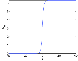
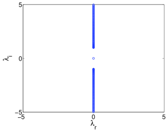
Figure 1: The left panel shows the profile $u_{0}$ of the kink of the sG model as a function of $x$. The right panel shows the spectral plane $(\lambda_{r},\lambda_{i})$ of the linearization eigenvalues $\lambda=\lambda_{r}+i\lambda_{i}$; see the detailed discussion in the text.

In a sense, one may think of the spectrum of the kinks as consisting of two separate “ingredients”. On the one hand, there is the point spectrum (which consists purely of the neutral mode at $\lambda=0$) which pertains to the coherent structure itself. On the other hand, there is the continuous spectrum which corresponds to the background on which the waveform “lives”. The background for the kink is the $0$ state on the left and the $2\pi$ on the right. For an anti-kink, where the opposite sign exists in the exponent of the right hand side of Eq. (5) (and which connects $2\pi$ with $0$), this is reversed. We note that the parsing of the spectrum into localized and extended segments is of particular relevance when considering e.g. the effect of collisions between kinks and anti-kinks and how these reflect the integrability of the dynamics through the well-known notion of elasticity of soliton collisions pgk01 .

Results for kinks and their spectrum in the case of the $\phi^{4}$ model are similar to the sG case. In particular, in the case of Eq. (3), the kink assumes the well-known form of the heteroclinic solution to the Duffing oscillator

$$u_{0}(x)=\tanh(x-x_{0}).$$ (11)

Once again, the invariance with respect to translations, and associated conservation law are present (a general feature of Klein-Gordon field theories of the form $u_{tt}=u_{xx}-V^{\prime}(u)$ for arbitrary field-dependent potentials $V(u)$). In this case as well, the linearized problem can be written in the form of an eigenvalue problem,

$$\lambda^{2}v=\left[\partial_{x}^{2}+2(1-3u_{0}^{2})\right]v.$$ (12)

Here the homogeneous steady states are $\pm 1$ and $0$, with the first two being stable with $\lambda=\pm i\sqrt{4+k^{2}}$, while the latter is unstable with $\lambda=\pm\sqrt{2-k^{2}}$.

The spectrum of the kink is also known in this case, although it is more complex than that of the sG problem. In particular, the neutral mode with $\lambda=0$ has an eigenfunction $v(x)=\sqrt{3/4}{\rm sech}^{2}(x-x_{0})$. The continuous spectrum pertains to the band $\lambda=\pm i\sqrt{4+k^{2}}$ (again, similarly to the underlying homogeneous problem) with the eigenfunctions

$$v^{(k)}=N_{k}e^{ikx}\left(3\tanh^{2}(x-x_{0})-1-k^{2}-3ik\tanh(x-x_{0})\right),$$ (13)

where $N_{k}^{-2}=4\pi(2(k^{2}/2+1)^{2}+k^{2}/2)$ sugi . However, the key difference of the spectrum of the $\phi^{4}$ kink from that of the sG is the presence of a point spectrum mode, corresponding to a localized eigenfunction, in the gap between the origin of the spectral plane and the continuous spectrum (see Fig. 2). This internal (often referred to also as shape) mode of the kink has an eigenvalue $\lambda=\pm\sqrt{3}i$ and a corresponding eigenfunction,

$$v(x)=\sqrt{\frac{3}{2}}\tanh(x-x_{0}){\rm sech}(x-x_{0}).$$ (14)

Figure 2: Same as Fig. 1, but now for the kink of the $\phi^{4}$ model. Notice on the right panel’s spectral plane the additional presence of the point spectrum eigenvalue at $\lambda=\pm i\sqrt{3}$.

It is this localized “shape” mode that has been argued to be typically responsible for the very rich phenomenology of collisions of $\phi^{4}$ kinks and anti-kinks as explored e.g. in anninos ; campbell ; campbell2 ; roy1 ; roy2 , among other works.

II.2 Anti-Continuum Limit and its Spectral Properties

We now turn to the opposite end of the continuum limit to construct a complementary picture of the kink existence and stability properties, so that we can connect the two in the next subsection. In particular, we focus now on Eqs. (2) and (4), which correspond to the discrete models. Here, one way to interpret $\epsilon$ (e.g. in applications such as coupled torsion pendula) is that of the spring constant linearly connecting adjacent such pendula. A way of interpretation closer to numerical analysis is that of adjacent nodes of a lattice, separated by a distance $\Delta x$, such that $\epsilon=1/\Delta x^{2}$. This represents then a finite difference scheme for the spatial discretization of the corresponding continuum models of Eqs. (1) and (3) and as such the continuum limit is approached when $\Delta x\rightarrow 0\Rightarrow\epsilon\rightarrow\infty$.

However, what was pioneered by MacKay and Aubry about 20 years ago macaub , was a technique that offered a completely alternative viewpoint to the one approaching the continuum as above. In particular, they advocated using the opposite limit, namely that of uncoupled oscillators at $\epsilon=0$. This was dubbed the anti-continuum (AC) limit. There, our system consists of isolated oscillators of the form $\ddot{u}_{n}=-\sin(u_{n})$ for the sG and $\ddot{u}_{n}=2(u_{n}-u_{n}^{3})$ for $\phi^{4}$. The steady states now are solely $0$ and $\pi$ (mod$(2\pi)$ as usual) and $\pm 1$ and $0$ for the two models, respectively. Hence one can think of ways to “initiate” a kink at this limit, which if $\epsilon$ starts becoming finite, upon continuation (using a bifurcation theory analogy), the kink will start gradually picking more sites progressively of more nontrivial ordinate. In this way, the kink will be progressively “fleshed out” (i.e., the spine of the heteroclinic connection will be populated) and will start looking more like its continuum analog, which will be eventually traced as $\epsilon\rightarrow\infty$. This kind of approach was used e.g. in balmf to construct a variety of kink and multi-kink solutions. Here, we will only explore the example of states leading (as $\epsilon$ is increased) to the single kink, and persisting from the AC to the continuum limit.

Upon some toying with the relevant background states, one realizes that there are two prototypical possibilities for creating such a kink. One of them concerns the so-called intersite-centered configuration, initiated at the AC limit through a sequence $(0,\dots,0,0,2\pi,2\pi,\dots,2\pi)$ in the sG and similarly $(-1,\dots,-1,-1,1,1,\dots,1)$ in the $\phi^{4}$. On the other hand, there is the onsite-centered configuration, which incorporates a point of the unstable steady state in the middle, namely $(0,\dots,0,0,\pi,2\pi,2\pi,\dots,2\pi)$ in the sG and similarly $(-1,\dots,-1,-1,0,1,1,\dots,1)$ in the $\phi^{4}$.

If we now examine such configurations in the AC limit, it will be straightforward to infer their stability since the linearization operator under the discretization becomes an infinite dimensional matrix operator (or from a computational perspective it is restricted to a finite but large number of nodes domain). In this setting the linearization Jacobian matrix will be tri-diagonal with the following diagonal and super/sub-diagonal elements:

$$J_{i,i}=-2\epsilon-V^{\prime}(u_{i}),\quad\quad J_{i,i+1}=J_{i,i-1}=\epsilon.$$ (15)

Here $V^{\prime}(u_{i})=-\cos((u_{0})_{i})$ for the sG and $V^{\prime}(u_{i})=2(1-3(u_{0})_{i}^{2})$ for the $\phi^{4}$. In the AC limit ($\epsilon=0$) the matrix becomes diagonal and it is evident that the eigenvalues $\lambda^{2}$ will be negative if the kink involves only the stable steady states ($0,2\pi$ or $\pm 1$) and will have as many unstable eigenvalue pairs as many sites there are at the unstable fixed points $\pi$ for the sG and $0$ for the $\phi^{4}$.

Now, the key question becomes what can we expect in terms of the kink stability as we depart from the AC limit, i.e., for finite $\epsilon$. To determine this, we resort to a well-known theorem for matrix eigenvalue problems, namely Gerschgorin’s theorem atkinson . In particular, if the order of the Jacobian matrix is $N$, the eigenvalues $\lambda^{2}$ thereof belong to the sets

$$Z_{i}=\{z\in C,\quad|z-J_{i,i}|<r_{i},\quad{\rm with}\quad r_{i}=\sum_{j=1,j\neq i}^{N}|J_{i,j}|\}.$$ (16)

Applying this to our setting, we find that $|\lambda^{2}+2\epsilon+V^{\prime}(u_{i})|\leq 2\epsilon$, which in turn implies

$$-V^{\prime}(u_{i})-4\epsilon\leq\lambda^{2}\leq-V^{\prime}(u_{i}).$$ (17)

In the case of the stable fixed points (at $0,2\pi$ or at $\pm 1$, respectively for the 2 models), this inequality properly outlines the edges of the continuous spectrum. Hence, this indicates stability for $N\rightarrow\infty$, at least for small $\epsilon$ of the inter-site centered kink.

However a critical point is that it also establishes the instability of the site-centered kink that always bears one site centered at $\pi$ or $0$ in the sG or, respectively, the $\phi^{4}$ case. For this eigenvalue, we have $1-4\epsilon\leq\lambda^{2}\leq 1$ for sG, while $2-4\epsilon\leq\lambda^{2}\leq 2$. Hence, this approach guarantees the instability of the onsite-centered kink for $\epsilon\leq 1/4$ for the sG problem and for $\epsilon\leq 1/2$ in the $\phi^{4}$ case.

We now turn to the merging of the two pictures in the subsection that follows.

II.3 Merging the two pictures

In the intermediate regime between the continuum limit of $\Delta x\rightarrow 0$ and $\epsilon\rightarrow\infty$ and the AC limit of $\Delta x\rightarrow\infty$ and $\epsilon\rightarrow 0$, we anticipate the following. For the site centered kink, we expect that the unstable eigenvalue, while bounded away from $0$ along the real line, according to our above estimate, will start approaching the origin of the spectral plane as the continuum limit is approached. While it is not guaranteed from our considerations herein that the eigenvalue will have a monotonic behavior, we find that indeed it does, only arriving at the origin as the asymptotic limit of the continuum regime is reached. The approach of this eigenvalue towards the spectral plane origin is shown in the left panel of Fig. 3.

On the other hand, in a similar manner, for the stable inter-site centered kink, the approach towards the continuum limit needs to involve an eigenvalue pair that approaches the origin as $\Delta x\rightarrow 0$ and the translational invariance is restored. Since in this case all eigenvalues initially start at $\pm i$ (at $\epsilon\rightarrow 0$) what occurs is that an eigenvalue pair bifurcates from the continuous spectrum and starts approaching the origin of the spectral plane. In this case too, although not necessarily so, the approach to the origin is monotonic (and asymptotic) as $\Delta x$ is decreased. This case is shown in the right panel of Fig. 3.

The eigenvalue associated to instability (resp. stability) of the site (resp. intersite) kinks is related to the translational invariance (TI) in the continuum limit. It is the breaking of the translational invariance once the system becomes discrete that is “responsible” for the instability/stability of these two different kinks. The difference in the energies associated to these two kinks is defined as the celebrated Peierls-Nabarro (PN) barrier, which is discussed at considerable length in the physical literature braun as the barrier needed to be overcome for a dislocation to move by a lattice site.

One of the typical issues that arise in the calculation of the PN barrier is that it is not straightforward to perturb off of the continuum limit in the direction of discreteness. This problem was bypassed in kk01 by perturbing off of an exceptional (translationally invariant) discretization of the sG model originally proposed by Speight and Ward in sw94 . This was in the form:

$$\ddot{u}_{n} = 2\epsilon\left(\sin(\frac{u_{n+1}-u_{n}}{2})-\sin(\frac{u_{n}-u_{n-1}}{2})\right)$$

$$- \frac{1}{2}\left(\sin(\frac{u_{n+1}+u_{n}}{2})+\sin(\frac{u_{n}+u_{n-1}}{2})\right).$$

The fact that this model is TI implies that it possesses kinks which can be located arbitrarily, as is in fact evidenced by the exact solutions $u_{n}=4\arctan(e^{a(n-\xi)})$ where $a=\log((2+\Delta x)/(2-\Delta x))$ and $\xi$ is a free parameter. It also suggests that the relevant TI eigenvalue pair is at $\lambda^{2}=0$, yet because of its inherent discrete nature, the model is amenable to being perturbed to be reshaped in the form of Eq. (3). Following this path, kk01 predicted that the relevant eigenvalue should be given by

$$\lambda_{r}\approx\pm\frac{13.96}{\Delta x^{1/2}}e^{-\frac{\pi^{2}}{\Delta x}},\quad\quad\lambda_{i}\approx\pm i\frac{13.96}{\Delta x^{1/2}}e^{-\frac{\pi^{2}}{\Delta x}}.$$ (19)

The first of these expressions applies to the real eigenvalue of the onsite-centered kink, while the second to the imaginary one of the intersite-centered kink. Both are applicable when approaching the continuum limit. Yet, it was recognized in kk01 that while the functional form of the dependence should be suitable, the prefactor may sustain additional contributions from higher order terms which should appear in the same order of eigenvalue dependence. It is for this reason that the dashed lines describing this theoretical dependence of Eq. (19) capture the appropriate functional dependence as the limit is approached, but clearly the prefactor is smaller than it should be.

Entirely similar features also arise for the $\phi^{4}$ case, which is thus not examined further here. Instead, we now turn to the corresponding examination of the breather waveform.

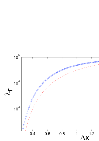
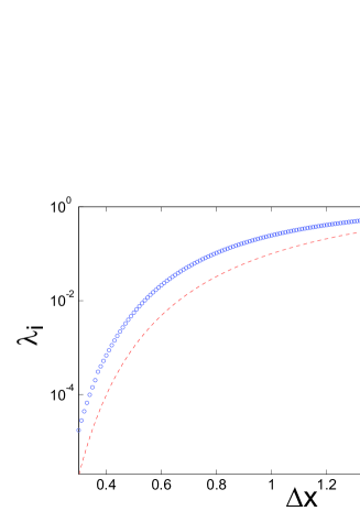
Figure 3: The left panel shows the real eigenvalue pertaining to the breaking of TI for the onsite centered kink. The blue symbols denote the numerical computation of this eigenvalue and the red dashed line provides the corresponding theoretical prediction of Eq. (19). The right panel shows the imaginary eigenvalue similarly associated to the breaking of TI for the stable intersite centered kink (the symbols/lines have the same designation as for the left panel).

III The Breather Case

The other fundamental solution of the sG model is a state which is also exponentially localized in space (similarly to the kink) but periodically varying in time. This is the so-called breather state whose exact profile is given by

$$u(x,t)=4\arctan\left(\sqrt{\frac{1-\omega^{2}}{\omega}}\sin(\omega(t-t_{0})){\rm sech}(\sqrt{1-\omega^{2}}(x-x_{0}))\right).$$ (20)

Aside from translations with respect to space and time (discussed in the previous section), this solution has a free parameter $\omega$, associated with the frequency of its “breathing” satisfying $0<\omega<1$. Interestingly, the breather seems like the result of the merger of a kink and an antikink, however although the energy of the kink and antikink is $8$ such that the sum of their energies is $E=16$, the energy of their bound state, i.e. the breather, is always less than that i.e., $E=16\sqrt{1-\omega^{2}}$.

III.1 Continuum limit: Genuine breathers and modulating pulses

For the sG equation, which is an infinite dimensional completely integrable Hamiltonian system, breather solutions can be obtained through its auto-Bäcklund transformation (BT). This procedure is, of course, limited to integrable systems and does not help in the quest for breathers in general (KG) equations

$$u_{tt}=u_{xx}-u+f(u)\,,$$ (21)

with $x,t,u=u(x,t)\in\mathbb{R},$ and some nonlinearity $f(u)$. To this end, various techniques have been employed and developed during the past decades to elucidate the existence of breathers or solutions akin to it. Roughly speaking, one can distinguish between three approaches. The first approach is the analysis via series expansion techniques (see kruskalseg ; kichenassamy ) and the study of perturbed sG equations (see birnir_mackean_weinstein ; denzler_93 ; denzler_97 ), whose findings indicated the non-persistence of breather families and the continuation of breathers as solutions which lack the spatial localization property. Out of these results emerged the more general second approach of constructing for (21) so-called modulating pulses, which are moving breathers that are not necessarily spatially localized, but feature oscillating tails; see e.g. groves_schneider ; shatah_zeng . Yet a different, third approach exploits the wave packet structure of breathers. In their small-amplitude limit they can be thought of as wave packets whose envelope is described by a Nonlinear Schrödinger (NLS) equation (see KirrmannSchneiderMielke for a rigorous approximation result). While perturbation arguments in the first approach rely heavily on integrable systems techniques and/or the explicit solution formula known for breathers, the second approach follows the realm of infinite dimensional dynamical systems and inspires an extension of center manifold theory beyond the classical case. The methodology of the third approach belongs to the theory of reduction to amplitude/modulation equations and plays an important role far beyond the setting discussed here.

Before we review each approach in more detail, let us briefly summarize the sG-breather construction. As alluded to, the sG equation admits an auto-Bäcklund transformation, which is, loosely speaking, a means of obtaining solutions to the sG equation by a procedure that is in some sense easier than solving a PDE (i.e. it might involve solving ODEs or algebraic equations). To be more precise, the BT maps “solutions to solutions”, i.e., it is a mapping $B$ with

$$B(u_{1};a)=u_{2}\,,\qquad u_{1},u_{2}\ \mathrm{solutions}\ \mathrm{of}\ \mathrm{(sG)}$$

where $a$ is some parameter. One can, for instance, use the trivial solution as a seed to grow non-trivial solutions like kinks or anti-kinks

$$B(0,1)=4\,\arctan(e^{x})\,,\qquad B(0,-1)=4\,\arctan(e^{-x})\,.$$ (22)

It is even possible to derive a surprisingly simple relation between four different solutions $u,U,u_{1},u_{2}$ of the (sG) equation by using the commutativity theorem schematically depicted in Figure 4 (cf., for instance, mclaughlin_scott ).

$$\tan\left(\frac{u+U}{4}\right)=\left(\frac{a_{1}+a_{2}}{a_{1}-a_{2}}\right)\,\tan\left(\frac{u_{1}+u_{2}}{4}\right)$$

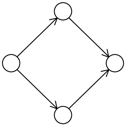
Figure 4: Scheme of commutativity of the BT: $B(B(u,a_{1}),a_{2})=B(B(u,a_{2}),a_{1})$

Using this scheme, one can derive a formula for (a family of) standing breathers (see Figure 5)

$$u_{*}(x,t;\omega)=4\,\arctan\left(\frac{m}{\omega}\,\frac{\sin(\omega t)}{\cosh(mx)}\right)\,,\quad m^{2}+\omega^{2}=1\,,$$ (23)

with $u=0,u_{1/2}=\mathrm{arctan}\left(e^{mx\pm i\omega t}\right)$ and $U=u_{*}$. Note that choosing $\omega=i\widetilde{\omega}\in i\mathbb{R}$ turns $u_{*}$ into

$$u_{*}(x,t;i\widetilde{\omega})=4\,\arctan\left(\frac{m}{i\widetilde{\omega}}\,\frac{\sin(i\widetilde{\omega}t)}{\cosh(mx)}\right)=4\,\arctan\left(\frac{m}{\widetilde{\omega}}\,\frac{\sinh(\widetilde{\omega}t)}{\cosh(mx)}\right),$$ (24)

which describes a kink/anti-kink solution (see Figure 5). Iterating this procedure results in more complicated solutions given by complexes of kinks and/or breathers.

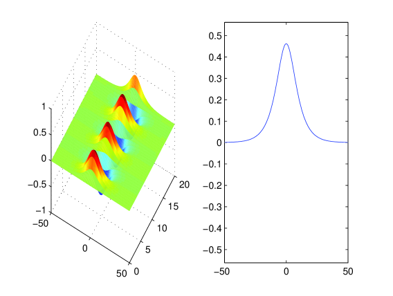
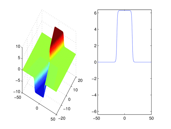
Figure 5: Top panel: Standing breather with $\omega=0.99$ in (23). Bottom panel: Kink/anti-kink interaction with $\omega=i0.99$ in (24).

As alluded to, one can derive kink solutions by a completely different viewpoint, namely, by making a traveling wave ansatz $u(x,t)=y\left(x-ct\right)\,,0\leq c<1\,,$ and examining the traveling wave ODE whose heteroclinics are given by $y(\xi)=4\,\arctan(e^{\pm\xi})\,,\xi=\gamma(x-ct)\,,\gamma=(1-c^{2})^{-1/2}$. For $c=0$ we recover (22), while the traveling kink can be viewed also as a consequence of the Lorentz transformation (7), as discussed above. Note, however, that breathers (or, more generally, any multikink solution) cannot be obtained from the traveling wave ODE since they are not stationary in any fixed co-moving frame. Hence, breathers can be viewed as genuinely infinite dimensional structures. While the explicit expressions (23) or (24) rely heavily on PDE tools for integrable systems, the general non-integrable case calls for different PDE techniques. Breather existence could, for instance, be explored via the construction of small-amplitude wave packets, which can be approximately performed for a large class of Klein-Gordon equations (21) via reduction to amplitude/modulation equations. Despite their widespread use, rigorous justifications of such procedures are more sparse, with an early example being KirrmannSchneiderMielke , where it was demonstrated that there are solutions $u$ to the (sG) equation for which

$$\sup_{t\in\left[0,\frac{T_{0}}{\varepsilon^{2}}\right]}\,||u(\cdot,t)-u_{\rm a}(\cdot,t)||_{C_{b}^{r}}\leq C\varepsilon^{3/2},$$

with $0<\varepsilon\ll 1$ being a small perturbation parameter and where $u_{\rm a}$ is a small-amplitude wave packet

$$u_{a}(x,t)=\varepsilon\,A(\varepsilon(x-\omega^{\prime}(k_{0})t),\varepsilon^{2}t)\,e^{ik_{0}x-i\omega(k_{0})t}+c.c.+h.o.t.\,,$$ (25)

with $\omega(k)=\sqrt{k^{2}+1}$; the envelope $A=A(X,T)\in\mathbb{C}$ is obtained by solving the Nonlinear Schrödinger (NLS) equation

$$2i\omega(k_{0})\partial_{T}A=(\omega^{\prime}(k_{0})^{2}-1)\partial^{2}_{X}A-3|A|^{2}A\,.$$ (26)

This result is also valid for general KG equations of the form given in (21) since small-amplitude solutions do not feel to leading order the exact structure of the nonlinearity. Note that, if we choose the NLS soliton as an envelope, the wave packet ansatz $u_{a}$ resembles the traveling sG breather in the small-amplitude limit $0<m=\varepsilon\ll 1$. Note that, although the approximation result treats a large class of solutions – namely, those whose envelopes are given by solutions of the NLS – of which the breather is just a special case, the limited time-validity of the construction (namely, $t\in\left[0,\frac{T_{0}}{\varepsilon^{2}}\right]$) does not give the optimal result (that is, global existence in time) in the breather case. Such an improvement of the perturbation procedure has so far not been reported in the literature and would be a particularly interesting direction for future work.

The analogy between breathers and general wave packets becomes even more remarkable when one considers interaction. Using the BT, one can construct, for instance, a 2-breather describing the elastic collision of two individual breathers. Such an interaction for small amplitude wave packets in the general KG setting (21) has striking similarities to the breather interaction: to leading order, the shape of the wave packets remains unchanged after collision, the only interaction effects being a shift of envelope and carrier waves (see ccsu for KG with constant coefficients and cs for KG with spatially periodic coefficients). In the case of large amplitudes, however, the situation is far more complex, as is attested also by the complexity of interactions of simpler structures such as kinks in non-integrable KG models belova ; anninos ; campbell ; campbell2 ; roy1 ; roy2 . Since a large class of KG equations support (approximate) small-amplitude wave packets which seem akin to the sG breather, it had been long speculated that exact breathers may exist for other KG equations as well. This belief has been proven wrong in numerous case examples from several different viewpoints.

The work of kruskalseg contrasted the sG setting with the $\phi^{4}$ model. By employing the Fourier representation

$$u(x,t)=\sum_{n\in\mathbb{Z}}\,\hat{u}_{n}(x)\,e^{in\omega_{*}t},$$ (27)

for time-periodic solutions with some temporal frequency $\omega_{*}/2\pi$, they derive an infinite-dimensional system of equations for the Fourier coefficients $\hat{u}_{n}$ and conclude that only the sG equation allows spatially localized solutions $\hat{u}_{n}(x)\rightarrow 0,x\rightarrow\pm\infty$, which in turn give rise to breathers, while the $\phi^{4}$ model only supports approximate breathers that slowly radiate their energy to $\pm\infty$.

The work of kichenassamy considered a more general KG setting with a force term $f(u)$ in (21) and presented a detailed convergence analysis of different breather series expansions relating the corresponding expansion coefficients to the coefficients $f_{n}$ in $f(u)=\sum_{n=1}^{\infty}f_{n}\,u^{n}$. The main result singles out the cases $f(u)=Cu,C\sinh(au),C\sin(au)$ which are the only choices yielding analyticity of the solution, while (again) only $f(u)=C\sin(au)$ gives breathers. In the early 90’s, the works of birnir_mackean_weinstein and denzler_93 ; denzler_97 studied perturbed sG equations

$$u_{tt}-u_{xx}+\sin(u)=\varepsilon P(u;\varepsilon)\,,\quad 0<\varepsilon\ll 1\,,$$ (28)

and concluded that breathers can persist (in families) if and only if the perturbation is equivalent to a rescaling of the sG equation. Consequently, the non-persistence results indicated that breathers perturb into solutions that are similar in nature, but not localized. This intuition was confirmed in groves_schneider (and later also in shatah_zeng ) by using spatial dynamics and a blend of invariant manifold, partial normal form and bifurcation theory for KG equations (21). They study so-called modulating pulse solutions, that is,

$$u(x,t)=v(x-(1/c_{\rm ph})t;x-\left(c_{\rm ph}+\gamma_{1}\varepsilon^{2}\right)t)=v(\xi,y),$$

where $v$ is periodic in $y$ with period $2\pi/k_{0}$ for some $k_{0}>0$. Note that the sG-breathers fall into this class with the additional property of being localized in $\xi$, a feature that seems rather exceptional in the following way. The infinite dimensional system for $(v,v_{x})$ on the phase space $\chi=\{(v,w)\in H_{\rm per}^{s+1}\times H_{\rm per}^{s}\},s\geq 0,$ (where now $x$ is the dynamic variable, hence, the name spatial dynamics and $H_{\rm per}^{s}$ are $L^{2}$-based Sobolev spaces of periodic functions) has a Hamiltonian structure whose linearization features infinitely many eigenvalues on the imaginary axis and exactly two real eigenvalues $\lambda_{1,2}=\pm\varepsilon\rho$. The leading order analysis of the full nonlinear system restricted to the subspace associated with $\lambda_{1,2}$ reveals a homoclinic which is, however, unlikely to persist for the full system. So, in general, one expects that resonances related to the infinitely many eigenvalues on the imaginary axis generate oscillatory tails, hence, preventing the existence of truly localized breathers for the full PDE. The special structure of the sG-nonlinearity seems to remedy this spectral picture, allowing the homoclinic to persist. Nevertheless, other mechanisms to avoid such resonances are possible in KG equations with e.g. periodic coefficients bcls .

III.2 Spectral Properties of the Breather: From the Anti-Continuum to Finite Coupling

In a chain of $N$ oscillators described by e.g. Eq. (2) or (4), discrete breathers in the AC limit consist of $p$ (excited) oscillators describing periodic orbits of frequency $\omega\neq\omega_{0}$ and $N-p$ oscillators at rest. Here, $\omega_{0}$ is the frequency of the oscillations at the linear limit around the equilibrium position $\tilde{u}$, with $\tilde{u}=0$ in the sine-Gordon and $\tilde{u}=\pm 1$ in the $\phi^{4}$ case. Breathers with $p>1$ are usually dubbed multibreathers; in the special case when $p=N$, they constitute an anharmonic phonon and are also known as phonobreathers. The MacKay–Aubry theorem macaub establishes that if $n\omega\neq\omega_{0}$ with $n$ being an integer, a time-reversible breather or multibreather can be continued to a nonzero coupling (i.e. $\epsilon\neq 0$). The time-reversible multibreather can be expressed as a Fourier series:

$$u_{n}(t)=\sum_{k=0}^{\infty}z_{k,n}\cos(k\omega t).$$ (29)

In the case of the sine-Gordon equation, due to the spatial symmetry of the potential, all the even coefficients are zero and the resonance condition mentioned above restricts to only odd multiples of $\omega$.

Among all the localized multibreathers supported by the lattice, there are only two that can be continued up to $\epsilon\rightarrow\infty$: (1) the single-site breather, i.e. the breather with $p=1$ (also known as the site-centered breather or Sievers–Takeno mode stak ), and (2) the two-site breather, i.e. multibreather with $p=2$, whose excited sites are adjacent and oscillate in phase, which is also dubbed as the bond-centered breather or Page mode page .

Very recently, it was proven that non-time-reversible multibreathers cannot exist in Hamiltonian lattices if the number of neighbors of each oscillator is equal to two and the boundary conditions are not periodic kouk3 . This proof does not forbid, however, the existence of non-time-reversible multibreathers in two-dimensional lattices where discrete vortices or percolating clusters kouk2 ; ijbc ; cretegny1 ; cretegny2 have been found in the past. In addition, non-time-reversible multibreathers have also been demonstrated in one-dimensional chains with periodic boundary conditions phason or long-range interactions kouk4 .

In order to obtain periodic orbits of the lattice equations (2) or (4), a fixed-point method (such as the Newton-Raphson method) can be implemented either in real or in Fourier space. In the real space case (see e.g. cretegny1 ), orbits are found as roots of the map $(\{u_{n}(T)\},\{\dot{u}_{n}(T)\})-(\{u_{n}(0)\},\{\dot{u}_{n}(0)\})$ with $T=2\pi/\omega$. The Jacobian of this map is $\mathcal{M}-I$ where $\mathcal{M}$ is the monodromy matrix (see e.g. (33)) and $I$ is the identity. Fourier space methods consist of introducing the Galerkin truncation to index $k_{m}$ of the Fourier series expansion (29) into the lattice equations so that they can be cast as a set of algebraic equations of the form phason :

$$-k^{2}z_{k,n}^{2}=\epsilon\Delta_{2}z_{k,n}-\mathcal{F}_{k,n},$$ (30)

with $\mathcal{F}_{k,n}$ being the discrete cosine Fourier transform,

$$\mathcal{F}_{k,n}=\frac{1}{N}\sum_{n=-k_{m}}^{k_{m}}V^{\prime}\left(\sum_{p=-k_{m}}^{k_{m}}z_{p,n}\cos\left[\frac{2\pi pn}{N}\right]\right)\cos\left[\frac{2\pi kn}{N}\right],$$ (31)

with $N=2k_{m}+1$ and $V^{\prime}(u)=\sin(u)$ for the sine-Gordon model and $V^{\prime}(u)=u^{3}-u$ for the $\phi^{4}$ equation. Fourier space methods have the advantage of providing with an analytical expression for the Jacobian, whereas it must be numerically generated by means of numerical integrators (as Runge-Kutta) in real space methods. On the contrary, the dimension of the Jacobian in Fourier space $[(k_{m}+1)N,(k_{m}+1)N]$ is larger than in the real space $(N,N)$ which makes the inversion intractable for large lattices.

Spectral stability of periodic orbits can be determined by means of Floquet analysis. This consists firstly of introducing a perturbation $\xi_{n}$ to a given solution $u_{n,0}$ of the lattice equations (2), (4). Then, the equation for the perturbation reads:

$$\ddot{\xi}_{n}=\epsilon\Delta_{2}\xi_{n}-V^{\prime\prime}(u_{n,0})\xi_{n},$$ (32)

with $V^{\prime\prime}(u_{n})=\cos u_{n}$ and $V^{\prime\prime}(u_{n})=3u_{n}^{2}-1$ for, respectively, the sine-Gordon and $\phi^{4}$ models. The stability properties are given by the spectrum of the Floquet operator $\mathcal{M}$ (whose matrix representation is called monodromy) defined as:

$$\left(\begin{array}[]{c}\{\xi_{n}(T)\}\\ \{\dot{\xi}_{n}(T)\}\\ \end{array}\right)=\mathcal{M}\left(\begin{array}[]{c}\{\xi_{n}(0)\}\\ \{\dot{\xi}_{n}(0)\}\\ \end{array}\right).$$ (33)

The $2N$ monodromy eigenvalues $\Lambda=\exp(\mathrm{i}\theta)$ are dubbed as Floquet multipliers and $\theta$ are denoted as Floquet exponents. Due to the symplectic nature of the Floquet operator for our Hamiltonian systems of interest, if $\Lambda$ is a multiplier, so is $\Lambda^{-1}$, and due to its real character if $\Lambda$ is a multiplier, so is $\Lambda^{*}$. Consequently, Floquet multipliers always come in complex quadruplets $(\Lambda,1/\Lambda,\Lambda^{*},1/\Lambda^{*})$ if $|\Lambda|\neq 1$ and is not real, or in pairs $(\Lambda,1/\Lambda)$ if $\Lambda$ is real, or $(\Lambda,\Lambda^{*})$ if $|\Lambda|=1$ and is not real. In addition, due to the time translation invariance of the system there is always a pair of multipliers at $+1$. Therefore, for a breather to be stable, all the multipliers must lie on the unit circle.

In the AC limit, Floquet multipliers lie in three bundles. The two conjugated ones, corresponding to the oscillators at rest, lie at $\theta=\pm 2\pi\omega_{0}/\omega$, while the third one lies at $+1$ and consists of $p$ multiplier pairs corresponding to the excited oscillators. For $\epsilon\neq 0$, the bundle corresponding to the oscillators at rest split and their multipliers move to form the phonon band, while the multipliers corresponding to the excited oscillators can move along, either in the unit circle (stability), or along the real axis (instability). However, as mentioned above, a pair of multipliers remains at $+1$ corresponding to the, so-called, phase and growth modes of the whole system. This implies that single-site breathers are stable for low coupling aubry .

Whereas the stability at low coupling of single-site breathers is trivial, the situation for multibreathers is less clear.

The theorems developed in mst ; kouk1 provide insight regarding this question. One can derive an expression of the Floquet multipliers corresponding to the excited oscillators of multibreathers close to the AC limit. In the case of Page modes, the relevant Floquet exponent is given by:

$$\theta=\pm\frac{2\pi}{\omega}\sqrt{2\epsilon\frac{J}{\omega}\frac{\partial\omega}{\partial J}},$$ (34)

with

$$J=\frac{1}{2\pi}\int_{0}^{T}[\dot{u}(t)]^{2}\mathrm{d}t=\frac{\omega}{2}\sum_{k\geq 1}k^{2}z_{k}^{2},$$ (35)

being the action of an isolated oscillator. Applying a rotating wave approximation (RWA) $u(t)\approx z_{0}+z_{1}\cos(\omega t)$ we obtain the following Fourier coefficients for the sG model abram :

$$z_{0}=0,\qquad z_{1}=12-4\sqrt{3[3-4(1-\omega^{2})]},$$ (36)

whereas the following coefficients are found for the $\phi^{4}$ model:

$$z_{0}=1-\frac{3}{5}(2-\omega^{2}),\qquad z_{1}=\frac{2}{5}(2-\omega^{2}).$$ (37)

Using the values from (34), the relevant Floquet exponent at low coupling for the sG model can now be approximated by:

$$\theta=\pm\frac{2\pi}{\omega}i\sqrt{2\epsilon\frac{\omega^{2}\sqrt{3(4\omega^{2}-1)}-(2\omega^{2}-1)(4\omega^{2}-1)}{16\omega^{4}-7\omega^{2}+1}},$$ (38)

whereas for the $\phi^{4}$ equation we have

$$\theta=\pm\frac{2\pi}{\omega}i\sqrt{2\epsilon\frac{\omega^{2}-2}{2-3\omega^{2}}}.$$ (39)

Figure 6 compares the Floquet exponents of the Page mode found by integrating the perturbation equation (33) with those of the analytical approximation (34) and the subsequent, fully analytical RWA (38)-(39) for low coupling. Good agreement is found in the case of small values of the coupling constant $\epsilon$.

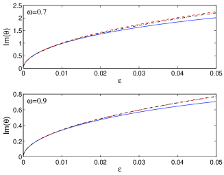
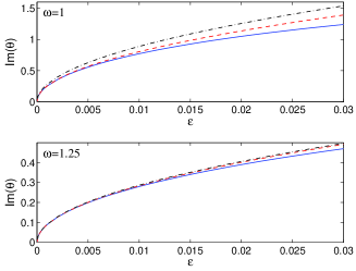
Figure 6: Floquet exponent for the Page mode in the sine-Gordon (left) and $\phi^{4}$ (right) models. Full line corresponds to the numerically exact result, whereas the stability theorem predictions are given by the dashed line. The explicit analytical predictions of the RWA approach for the stability exponents are depicted by the dash-dotted line.

III.3 Continuation in the Coupling: Going towards the Continuum

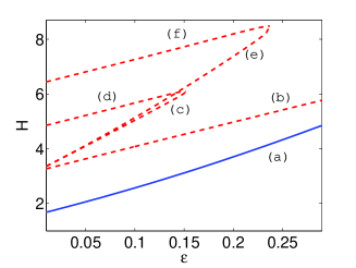
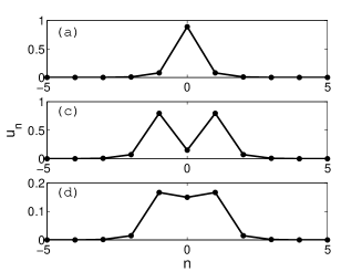
Figure 7: Left: Hamiltonian energy (H) of breathers of the discrete sG equation as the coupling parameter $\epsilon$ is increased for $\omega=0.7$. The labels correspond to breathers which have the following excited nodes in the AC limit: (a) $(\ldots,\bullet,\bullet,\bullet,\uparrow,\bullet,\bullet,\bullet,\ldots)$ (b) $(\ldots,\bullet,\bullet,\bullet,\uparrow,\uparrow,\bullet,\bullet,\ldots)$ (c) $(\ldots,\bullet,\bullet,\uparrow,\bullet,\uparrow,\bullet,\bullet,\ldots)$ (d) ($\ldots,\bullet,\bullet,\uparrow,\uparrow,\uparrow,\bullet,\bullet,\ldots$) (e) $(\ldots,\bullet,\bullet,\uparrow,\bullet,\bullet,\uparrow,\bullet,\bullet,\ldots)$ and (f) $(\ldots,\bullet,\bullet,\uparrow,\uparrow,\uparrow,\uparrow,\bullet,\bullet,\ldots$). Here, arrows correspond to the excited sites, which oscillates with frequency $\omega$, whereas the oscillators at rest are represented by dots. Only the site-centered (a) and bond-centered (b) solutions survive for $\epsilon\rightarrow\infty$, both of which approach the exact breather solution of the continuous sG equation, see Eq. (20). Right: Examples of discrete sG breathers for $\epsilon=0.065$. The multibreathers in the two bottom panels collide in a fold bifurcation at $\epsilon\approx 0.152$. The labels correspond to those in the left panel.

When the coupling constant is increased to finite values of $\epsilon>0$, stable multibreathers that are close to the AC limit destabilize generally by means of Hamiltonian Hopf bifurcations (also referred to as Krein crunches); in addition, every multibreather ceases to exist for a finite value of the coupling constant by means of Hopf or fold bifurcations. As discussed above, the two exceptions to these facts are given by the Sievers-Takeno (site-centered breathers) and Page modes (bond-centered breathers) which can be continued up to the continuum limit ($\epsilon\rightarrow\infty)$. During this continuation, however, both modes experience important changes both in their shape and in their spectral properties, as we will see below.

The site-centered and bond-centered modes can be continued until resonance with the linear phonon band occurs. For periodic boundary conditions and assuming that the lattice has an even number of particles $N$, the phonon band is given by:

$$\omega^{2}_{\mathrm{ph}}(\epsilon)=\omega_{0}^{2}+4\epsilon\sin^{2}\frac{q}{2},\qquad\mathrm{with}\qquad q=\left(1-\frac{2n}{N}\right)\pi,\ n=0,1,2\ldots N/2$$ (40)

where the modes are sorted by frequency and those from $n=1$ to $n=N/2-1$ are doubly degenerate; $\omega_{0}^{2}=1$ ($\omega_{0}^{2}=2$) in the sG ($\phi^{4}$) model. Therefore, the first resonance, upon variation of $\epsilon$ for fixed $\omega$, must occur when $n=0$, i.e. with the $q=\pi$ linear mode. In the case of $\phi^{4}$ potential, resonances occur when the second harmonic of the breather frequency coincides with a phonon frequency ($m\omega=\omega_{\mathrm{ph}}$, $m=2$), i.e. the first resonance occurs at $\epsilon_{\pi}=\omega^{2}-1/2$. However, in the sine-Gordon potential, the Fourier coefficients corresponding to even harmonics are zero, so that the resonance is caused by the third harmonic ($m\omega=\omega_{\mathrm{ph}}$, $m=3$) and the first resonance is observed at $\epsilon_{\pi}=(9\omega^{2}-1)/4$.

Thus, if a smooth continuation is performed, the site- (or bond-) centered solution continuously transforms into a phonobreather (i.e., resonates with the linear modes) once the coupling reaches the value $\epsilon_{\pi}$. The central site(s) will oscillate with frequency $\omega$ whereas the tail will oscillate with frequency $m\omega$. Nevertheless, if the step in the continuation method is large enough, the system is able to “jump” to a localized solution whose frequency lies in the gaps of the phonon band. Those solutions are the result of a hybridization of a breather with a phonon and are dubbed as phantom breathers phantom . Phantom breathers are in fact the discrete version of the nanopterons observed in the continuum $\phi^{4}$ equation boyd . However, unlike the continuum models, they typically arise for on-site potentials (including e.g. the discrete sine-Gordon) as long as the coupling is finite and higher than $\epsilon_{\pi}$. Similarly to nanopterons and the phonobreathers found by smooth continuation, phantom breathers are composed of a localized breather oscillating with frequency $\omega$ plus a low-amplitude background of frequency $m\omega$.

Let us mention that the bifurcation diagram for phantom breathers (see phantom for an extensive study of such solutions) resembles the Wannier–Stark ladders observed in a model of non-homogenous waveguide arrays wsl [see Fig. 8 (left)]; this implies the existence of three nonlinear modes for the same value of the coupling constant. Of course, the width of gaps in the phonon band decreases with the number of system particles $N$, and the gaps eventually vanish for $N\rightarrow\infty$. In other words, the hybridization of the breather with the background phonons is a finite-size artifact that disappears in the infinite lattice limit.

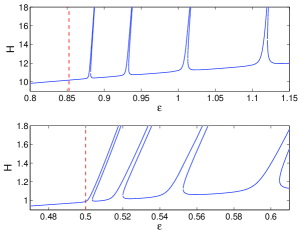
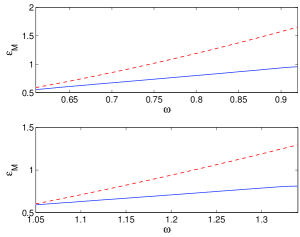
Figure 8: (Left panel) Hamiltonian energy versus coupling for breathers with frequency $\omega=0.7$ in the sine-Gordon model (top) and $\omega=1$ for the $\phi^{4}$ model (bottom). The vertical dashed line indicates the value $\epsilon_{\pi}$. (Right panel) Exchange of stability bifurcation loci for breathers in the sG (top) and $\phi^{4}$ potential (bottom); the dashed line indicates the value of $\epsilon_{\pi}(\omega)$.

Similar to the kink situation described in Sec. II.3, there are important details regarding the spectral properties of discrete breathers in the $\phi^{4}$ and sine-Gordon lattices. In both models, the site- and bond-centered modes interchange their stability at a finite value of the coupling constant, which we denote as $\epsilon_{M}$. This exchange-of-stability bifurcation (which is mediated by an intermediate breather) is closely related to the existence of moving breathers chen ; cretegny3 . This bifurcation is caused by a spatially anti-symmetric internal mode called pinning mode. For the site-centered breather mode, this internal mode detaches from the phonon band and becomes localized when $\epsilon$ is increased, colliding at $\theta=0$ when the exchange of stability takes place. In addition, moving breathers not only exist close to the parameter values at which stability exchange takes place but also when the Floquet multiplier corresponding to the pinning mode is close to 1. In this case, the movement is possible because the height of the Peierls–Nabarro barrier is related to the distance of the unstable multiplier to 1. Figure 8 (right) shows the dependence of $\epsilon_{M}$ with respect to $\omega$. In general, when $\epsilon$ becomes larger than $\epsilon_{M}$ the growth rate (distance of the unstable Floquet multiplier to 1) of the Sievers-Takeno mode grows up to a maximum value; beyond that point, there are many windows where stability exchanges again. Those windows correspond to the jumps into the phonon band and are difficult to control in the numerics. Nevertheless, as we approach $\epsilon\rightarrow\infty$, i.e., at the continuum limit, the relevant translational eigenvalue returns to the point $(1,0)$ of the unit circle, signaling the restoration of the translational invariance in that limit.

IV A Recent Variant: sine-Gordon Equations with $\mathcal{PT}$ Symmetry

One of the interesting recent extensions that have emerged in the context of Klein-Gordon field theories is that of $\mathcal{PT}$-symmetric variants of these models. The analysis of Hamiltonians respecting the concurrent application of parity ($x\rightarrow-x$) and time-reversal ($t\rightarrow-t$) operations was initially proposed in a series of publications by Bender and collaborators bend1 ; bend2 ; bend3 . While originally intended for Schrödinger Hamiltonians as a modification/extension of quantum mechanics, its purview has gradually become substantially wider. This stemmed to a considerable degree from the realization that other areas such as optics might be ideally suited not only for the theoretical study of this theme ziad ; Ramezani ; Muga , but also for its experimental realization salamo ; dncnat ; whisper . Recently, both at the mechanical level bend_mech and at the electrical one R21 ; tsampas2 realizations of $\mathcal{PT}$ symmetry and its breaking have arisen, while a Klein-Gordon setting has also been explored theoretically for so-called $\mathcal{PT}$ symmetric nonlinear metamaterials and the formation of gain-driven discrete breathers therein tsironis .

These efforts have, in turn, prompted a number of works both at the discrete level ptkg ; demirkaya , as well as at the continuum one demirkaya ; demirkaya2 to identify prototypical settings of application of $\mathcal{PT}$-symmetry in nonlinear KG field theories. The model used in demirkaya ; demirkaya2 is of the form:

$$u_{tt}-u_{xx}+\epsilon\gamma(x)u_{t}+f(u)=0.$$ (41)

Here, in order to preserve the $\mathcal{PT}$ symmetry, $\gamma(x)$, should be an antisymmetric function satisfying $\gamma(-x)=-\gamma(x)$. Physically, this implies that while this is an “open” system with gain and loss, the gain balances the loss, in preserving the symmetry.

Interestingly, for this class of models, the stationary states $u_{0}$, such as the kinks, are unaffected by the presence of the $\mathcal{PT}$ symmetry (since the relevant term involves $u_{t}$). On the other hand, the linearization problem becomes

$$\lambda^{2}v+\epsilon\lambda\gamma v+Hv=0.$$ (42)

where $H$ is the Hamiltonian linearization operator of e.g. Eqs. (9) or (12). Equivalently, the spectral problem can be written as:

$$\lambda\left(\begin{array}[]{c}v_{1}\\ v_{2}\end{array}\right)=\left(\begin{array}[]{cc}0&1\\ -H&-\epsilon\gamma(x)\end{array}\right)\left(\begin{array}[]{c}v_{1}\\ v_{2}\end{array}\right).$$ (43)

Now, the key question becomes what will be the fate of the eigenstates associated with the linearization around the continuum kink, in the presence of the perturbation imposed by the $\mathcal{PT}$-symmetric gain/loss term. What has been argued in demirkaya ; demirkaya2 is that in both the continuum and the infinite lattice discrete problem, the continuous spectrum will not be altered. Hence, the question is what becomes of the point spectrum in the presence of this perturbation.

To determine what happens to the mode associated with translation, we project Eq. (42) to the eigenfunction of vanishing eigenvalue (in the unperturbed limit $v=u_{0,x}$), and observe that the last term in Eq. (42) disappears. Assuming a perturbative expansion of $v$ in $\epsilon$, which to leading order (when $\epsilon=0$) has $v=u_{x}$, leads immediately to the leading order approximation

$$\lambda=0\quad{\rm or}\quad\lambda=-\epsilon\frac{\int\gamma(x)u_{0,x}^{2}dx}{\int u_{0,x}^{2}dx}.$$ (44)

This explicit expression should yield a fairly accurate prediction of the fate of the former double $0$ eigenvalue pair. Interpreting this result, we find that one of the two eigenvalues of the pair should remain at $0$ (a result that persists to all orders in perturbation theory due to the remaining invariance of the location of the solution under translations). On the other hand, the fate of the second eigenvalue will depend on the relative position of the kink centered at $x_{0}$ with respect to the origin. In particular, for both the sine-Gordon and the $\phi^{4}$, we find that if the kink is centered at the lossy side (say, $x_{0}<0$), then the numerator of the expression in Eq. (44) is negative, leading the second eigenvalue to the left hand plane. Reversing the sign of $x_{0}$ leads effectively to a reversal of the time flow (due to the nature of the system) and results into the corresponding eigenvalue moving by an equal amount to the right half of the spectral plane i.e., yielding instability. On the other hand, for the special case in which $x_{0}=0$, the parity of the relevant integral makes it vanish and the eigenvalue does not shift. A typical example showcasing the quality of the agreement of the theoretical prediction with full numerical results is shown in Fig. 9.

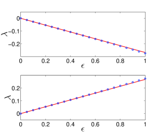
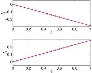
Figure 9: A typical example of the comparison of the motion of the translational eigenvalue under a $\mathcal{PT}$-symmetric perturbation between numerics (points) and analytics of Eq. (44). The left is for sG and the right for $\phi^{4}$, the top for a kink centered at the lossy side, while the bottom for a kink centered at the gain side.

However, in the case of the $\phi^{4}$ model, it is not sufficient to consider only the fate of the eigenvalue potentially bifurcating from the origin of the spectral plane. Recall that there is an eigenvalue at $\lambda^{2}=-3$. One can consider a perturbative expansion of such an eigenvalue in the problem, according to $\lambda=\lambda_{0}+\epsilon\lambda_{1}+\dots$, while $v=v_{0}+\epsilon v_{1}+\dots$. Applying a solvability condition at the leading order of the perturbation theory then immediately yields the eigenvalue leading order correction as:

$$\lambda_{1}=-\frac{1}{2}\frac{\int\gamma(x)v_{0}^{2}dx}{\int v_{0}^{2}dx}.$$ (45)

The interpretation of this result is that this isolated point spectrum eigenvalue (pair) will also move to the left half plane, for the case of the kink centered at the lossy side, while it will move (as a complex pair) to the right half plane when the kink is centered at the gain side. I.e., overall stability of the kink’s point spectrum is ensured when centered at the lossy region and instability when centered at the gain region. When the kink is at the interface, it should already be clear from the above considerations that all real contributions to the eigenvalue will vanish, allowing only imaginary ones that could shift the point spectrum along the imaginary axis, as proved earlier in the text. Again, very good agreement between this prediction and the full numerical result was found in demirkaya2 .

In the discrete case, the same methods as explored above yield equally accurate predictions. Arguably, the only significant modification arising here is in the case of the intersite centered stable kink. For the onsite one, the perturbation shifts the eigenvalue along the real axis (weakly, for small perturbation strength), not changing the fate of the kink’s (in)stability. However, in the marginal case of the intersite centered kink, once again, the lossy side leads to stability kicking the former translational (now imaginary in the discrete problem) eigenvalues to the left half-plane. Placing the kink on the gain side has the opposite effect with eigenvalues bifurcating on the right half plane (as a complex pair) and hence leading to instability. It is for that reason that the fate of the unstable discrete kink of the dynamical example of Fig. 10 leads to a static intersite centered structure on the lossy (left) side for the left panel of the figure. If, however, the perturbation pushes (intentionally) the kink toward the right hand (gain) side, it cannot find a stable equilibrium point and instead it continues to propagate as is shown in the right panel of the figure.

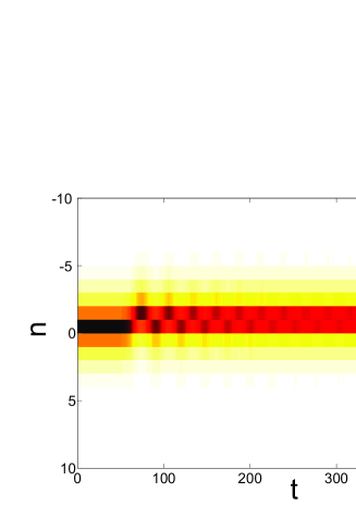
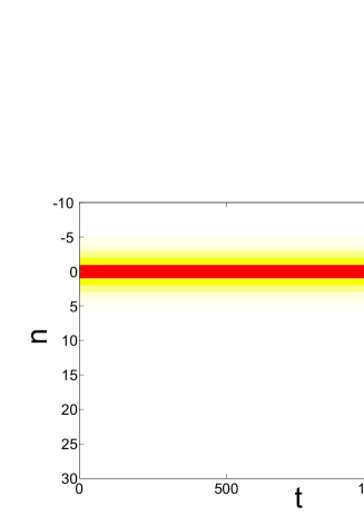
Figure 10: Two canonical examples of the evolution of an unstable kink on the gain side of a discrete $\mathcal{PT}$-symmetrically perturbed sG model. The left panel shows the kink as settling into an intersite-centered structure on the lossy side, while the right forces it to propagate on the gain side, but without bearing a stable fixed point for the kink state. Color bar represents $|u_{n}-\pi|$.

In the case of breathers, we can add that also based on the discussion given earlier for different variants of the sG equation and KG equations more generally, breathers are unlikely to exist under PT-symmetric perturbations. However, we do find that in the case example potentials that we considered, stationary breather solutions can only be found to exist at the delicate interface between gain and loss. Breathers seeded on the lossy side are found to become mobile. Perhaps more interestingly, such structures on the gain side appear to gain energy and transform themselves into a kink-antikink pair.

References

- (1) R.K. Dodd, J.C. Eilbeck, J.D. Gibbon, H.C. Morris, Solitons and Nonlinear Wave Equations (Academic Press, New York, 1983)
- (2) T. Dauxois, M. Peyrard, Physics of Solitons (Cambridge University Press, Cambridge, 2006)
- (3) M. Cirillo, R.D. Parmentier, B. Savo, Physica D 3, 565 (1981)
- (4) W.P. Su, J.R. Schrieffer, Phys. Rev. Lett. 46, 738 (1981)
- (5) A.R. Bishop, S.E. Trullinger, J.A. Krumhansl Physica D 1, 1 (1980)
- (6) J. Frenkel and T. Kontorova, J. Phys. 1, 137 (1939)
- (7) O.M. Braun, Yu.S. Kivshar, The Frenkel-Kontorova Model: Concepts, Methods and Applications (Springer-Verlag, Berlin, 1998)
- (8) A.C. Scott, Am. J. Phys. 37, 52 (1969)
- (9) A.C. Scott, Nonlinear Science, 2nd edn. (Oxford University Press, New York, 2003); A. Barone, F. Esposito, C.J. Magee, A.C. Scott, Riv. Nuovo Cim. 1, 227, 1971
- (10) J. Cuevas, L.Q. English, P.G. Kevrekidis, M. Anderson, Phys. Rev. Lett. 102, 224101 (2009)
- (11) M. Kimura, T. Hikihara, Chaos 19, 013138 (2009)
- (12) M.J. Ablowitz, H. Segur, Solitons and the Inverse Scattering Transform, (SIAM, Philadelphia, 1981)
- (13) T.I. Belova, A.E. Kudryavtsev, Phys. Usp. 40, 359 (1997)
- (14) P. Anninos, S. Oliveira, R.A. Matzner, Phys. Rev. D 44, 1147 (1991)
- (15) D.K. Campbell, J.F. Schonfeld, C.A. Wingate, Physica D 9, 1 (1983)
- (16) D.K. Campbell, M. Peyrard, Physica D 18, 47 (1986)
- (17) R.H. Goodman, R. Haberman, SIAM J. Appl. Dyn. Sys. 4, 1195 (2005)
- (18) R.H. Goodman, Chaos 18, 023113 (2008)
- (19) A.J. Heeger, S. Kivelson, J.R. Schrieffer, W.P. Su, Rev. Mod. Phys. 60, 781 (1988)
- (20) V.K. Wadhawan, Introduction to Ferroic Materials (Gordon and Breach, Amsterdam, 2000)
- (21) C.M. Bender, S. Boettcher, Phys. Rev. Lett. 80, 5243 (1998)
- (22) C.M. Bender, S. Boettcher, P.N. Meisinger, J. Math. Phys. 40, 2201 (1999)
- (23) C. M. Bender, Rep. Prog. Phys. 70, 947 (2007)
- (24) P.G. Kevrekidis, Phys. Lett. A 285, 383 (2001)
- (25) T. Sugiyama, Prog. Theor. Phys. 61, 1550 (1979)
- (26) R.S. MacKay, S. Aubry, Nonlinearity 7, 1623 (1994)
- (27) N.J. Balmforth, R.V. Craster, P.G. Kevrekidis, Physica D 135, 212 (2000)
- (28) K.E. Atkinson, An Introduction to Numerical Analysis, 2nd edn. (John Wiley and Sons, New York, 1989)
- (29) T. Kapitula, P. Kevrekidis, Nonlinearity 14, 533 (2001)
- (30) J.M. Speight, R. Ward, Nonlinearity 7, 475 (1994)
- (31) H. Segur, M.D. Kruskal, Phys. Rev. Lett. 58, 747 (1987)
- (32) S. Kichenassamy, Comm. Pure Appl. Math. 44, 789 (1991)
- (33) B. Birnir, H. McKean, A. Weinstein, Comm. Pure Appl. Math. 47, 1043 (1994)
- (34) J. Denzler, Comm. Math. Phys. 158, 397 (1993)
- (35) J. Denzler, Ann. Inst. H. Poincaré Anal. Non Linéaire 12, 201 (1995)
- (36) M.D. Groves, G. Schneider, Comm. Math. Phys. 219, 489 (2001)
- (37) J. Shatah, C. Zeng, Nonlinearity 16, 591 (2003)
- (38) P. Kirrmann, G. Schneider, A. Mielke, Proc. R. Soc. Edinb. Sect. A-Math. 122, 85 (1992)
- (39) D.W. McLaughlin, A.C. Scott, J. Math. Phys. 14, 1817 (1973)
- (40) M. Chirilus-Bruckner, Ch. Chong, G. Schneider, H. Uecker, Math. Anal. Appl. 347, 304 (2008)
- (41) M. Chirilus-Bruckner, G. Schneider, J. Diff. Eq. 253, 2161 (2012)
- (42) C. Blank, M. Chirilus-Bruckner, V. Lescarret, G. Schneider, Comm. Math. Phys. 302, 815 (2011)
- (43) A.J. Sievers, S. Takeno, Phys. Rev. Lett. 61, 970 (1988)
- (44) J.B. Page, Phys. Rev. B 40, 7835 (1990)
- (45) V. Koukouloyannis, Phys. Lett. A 377, 2022 (2013)
- (46) V. Koukouloyannis, R.S. MacKay, J. Phys. A: Math. Gen. 38), 1021 (2005)
- (47) J. Cuevas, V. Koukouloyannis, P.G. Kevrekidis, J.F.R. Archilla, Int. J. of Bif. & Chaos 21, 2161 (2011)
- (48) T. Cretegny, S. Aubry, Phys. Rev. B 55, R11929 (2007)
- (49) T. Cretegny, S. Aubry, Physica D 113, 162 (2008)
- (50) J. Cuevas, J.F.R. Archilla, F.R. Romero, J. Phys. A: Math. Theor. 44, 035102 (2011)
- (51) V. Koukouloyannis, J. Cuevas, P.G. Kevrekidis, V. Rothos, Physica D 242, 16 (2013)
- (52) J. Boyd, Nonlinearity 3, 177 (1990)
- (53) S. Aubry, Physica D 103, 201 (1997)
- (54) J.F.R. Archilla, J. Cuevas, B. Sánchez-Rey, A. Álvarez, Physica D 180, 235 (2003)
- (55) V. Koukouloyannis, P.G. Kevrekidis, Nonlinearity 22, 2269 (2009)
- (56) M. Abramowitz, I.A. Stegun, Handbook of Mathematical Functions, (Courier Dover Publications, 1964)
- (57) A.M. Morgante, M. Johansson, S. Aubry, G. Kopidakis, J. Phys. A: Math. Gen. 35, 4999 (2002)
- (58) T. Pertsch, U. Peschel, F. Lederer, Phys. Rev. E 66, 066604 (2002)
- (59) D. Chen, S. Aubry, G.P. Tsironis, Phys. Rev. Lett. 77, 4776 (1996)
- (60) S. Aubry, T. Cretegny, Physica D 119, 34 (1998)
- (61) Z.H. Musslimani, K.G. Makris, R. El-Ganainy, D.N. Christodoulides, Phys. Rev. Lett. 100, 030402 (2008)
- (62) H. Ramezani, T. Kottos, R. El-Ganainy, D.N. Christodoulides, Phys. Rev. A 82, 043803 (2010)
- (63) A. Ruschhaupt, F. Delgado, J.G. Muga, J. Phys. A: Math. Gen. 38, L171 (2005)
- (64) A. Guo, G.J. Salamo, D. Duchesne, R. Morandotti, M. Volatier-Ravat, V. Aimez, G. A. Siviloglou, D. N. Christodoulides, Phys. Rev. Lett. 103, 093902 (2009)
- (65) C.E. Rüter, K.G. Makris, R. El-Ganainy, D.N. Christodoulides, M.Segev, D. Kip, Nature Physics 6 (2010) 192
- (66) B. Peng, S.K. Ozdemir, F. Lei, F. Monifi, M. Gianfreda, G.L. Long, S. Fan, F. Nori, C.M. Bender, L. Yang, Nonreciprocal light transmission in parity-time-symmetric whispering-gallery microcavities, arXiv:1308.4564.
- (67) C.M. Bender, B.J. Berntson, D. Parker, E. Samuel, Am. J. Phys. 81, 173 (2013).
- (68) J. Schindler, A. Li, M. C. Zheng, F. M. Ellis, T. Kottos, Phys. Rev. A 84, 040101 (2011).
- (69) H. Ramezani, J. Schindler, F. M. Ellis, U. Günther, T. Kottos, Phys. Rev. A 85, 062122 (2012).
- (70) N. Lazarides, G. P. Tsironis, Phys. Rev. Lett. 110, 053901 (2013).
- (71) J. Cuevas, P.G. Kevrekidis, A. Saxena, A. Khare, Phys. Rev. A 88, 032108 (2013).
- (72) A. Demirkaya, D. J. Frantzeskakis, P. G. Kevrekidis A. Saxena, A. Stefanov, Phys. Rev. E 88, 023203 (2013).
- (73) A. Demirkaya, M. Stanislavova, A. Stefanov, T. Kapitula, P.G. Kevrekidis, Spectral stability of kinks in -symmetric Klein-Gordon, arXiv:1402.2942.