Construction of the B88 exchange-energy functional in two dimensions

Abstract

We construct a generalized-gradient approximation for the exchange-energy density of finite two-dimensional systems. Guided by non-empirical principles, we include the proper small-gradient limit and the proper tail for the exchange-hole potential. The observed performance is superior to that of the two-dimensional local-density approximation, which underlines the usefulness of the approach in practical applications.

1 Introduction

Nanoscale electronic devices define a large variety of low-dimensional systems that range from atomistic to artificial structures. These include, e.g., modulated semiconductor layers and surfaces, quantum Hall systems, spintronic devices, quantum dots ¹ (QDs), quantum rings, and artificial graphene. ² The complex effects of electron-electron interactions pose a challenge to accurately compute the energy components of these structures.

Density-functional theory ^{4, 5, 3} (DFT) is ideally suited to balance numerical effort and accuracy. Considerable advances beyond the commonly used local-density approximation (LDA) have been achieved by generalized gradient approximations (GGAs), orbital functionals, and hybrid functionals ⁶. Previous studies have shown that most functionals developed for 3D systems break down when applied to realistic models of two-dimensional (2D) systems. ^{7, 8} In particular, accurate modeling of semiconductor quantum dots (in, e.g. GaAs/AlGaAs interfaces ¹) requires the use of 2D functionals, since the degrees of freedom are suppressed in the direction perpendicular to the plane. The relevance of including in standard 3D functionals the ability to recover the 2D limit – at least at the LDA level – has been clearly demonstrated in a recent work dealing with heterogeneous 3D atomistic materials. ⁹ The construction of more elaborated approximations for the exchange-correlation energy in 2D beyond LDA ^{10, 11, 12} started also relatively recently ^{13, 14, 15, 16, 17, 18}; in particular, they demonstrated some of the limitations of the 2D-LDA and how to overcome them.

In this work we focus on exchange energies of finite systems and take the natural step beyond LDA by including the dependence of the functional on density gradients. We follow a procedure which solves the long-standing challenge of obtaining an non-empirical gradient expansion for the exchange energy of finite 2D systems. ¹⁹ We achieve this result by carrying out a semiclassical analysis analogous to that of high-Z atoms in 3D. ^{21, 20} The form of the functional used as a paradigm is B88. ²¹ This allows us not only to come up with a form that has a proper small-gradient expansion, but also to obtain a model for the exchange-hole potential that has the proper asymptotic tail.

The present work is organized as follows. In Sec. 2 we briefly review the construction of the B88 functional (in 3D) and then proceed with the 2D case, exploiting the semiclassical limit of parabolic quantum dots. In Sec. 3 we test the derived functional for a large set of QDs and quantum rings. A summary is given in Sec. 4.

2 Construction of B88 in two dimensions

2.1 General considerations

The functional known as B88 in 3D is – as a fundamental ingredient of B3LYP ²⁵ – among the most popular density functionals. It defines the energy density per electron with appealing features for finite systems such as a proper tail, ²¹ and it recovers an appropriate small-gradient limit. ^{21, 20}

Let us first briefly remind of the B88 expression in 3D. For (globally collinear) spin-polarized states, it is convenient to write the exchange energy in terms of the exchange-hole potential $U_{{\rm X},\sigma}$ as

$$E^{\rm B88}_{\rm X}=\frac{1}{2}\sum_{\sigma}\int d^{3}r~{}n_{\sigma}({\bf r})U^{\rm B88}_{{\rm X},\sigma}({\bf r})$$ (1)

and split it into two contributions

$$U^{\rm B88}_{{\rm X},\sigma}({\bf r})=U^{\rm LDA}_{{\rm X},\sigma}({\bf r})+\Delta U^{\rm B88}_{{\rm X},\sigma}({\bf r}).$$ (2)

Here the first term comes from the LDA,

$$U^{\rm LDA}_{{\rm X},\sigma}=C_{\rm X}n^{1/3}_{\sigma},~{}~{}C_{\rm X}=-3\left[\frac{3}{4\pi}\right]^{1/3},$$ (3)

and the second term is introduced in order to account for the inhomogeneities of the system through an expression

$$\Delta U^{\rm B88}_{{\rm X},\sigma}=-\beta\frac{n^{1/3}_{\sigma}x^{2}_{\sigma}}{1+6\beta x_{\sigma}\sinh^{-1}(x_{\sigma})},$$ (4)

that depends on the dimensionless gradient

$$x_{\sigma}=\frac{|\nabla n_{\sigma}|}{n^{4/3}_{\sigma}}\;.$$ (5)

A straightforward dimensional analysis suggests the following 2D version

$$E^{\rm 2D-B88}_{\rm X}=\frac{1}{2}\sum_{\sigma}\int d^{2}r~{}n_{\sigma}({\bf r})U^{\rm 2D-B88}_{{\rm X},\sigma}({\bf r}),$$ (6)

where

$$U^{\rm 2D-B88}_{{\rm X},\sigma}({\bf r})=U^{\rm LDA}_{{\rm X},\sigma}({\bf r})+\Delta U^{\rm 2D-B88}_{{\rm X},\sigma}({\bf r})\;,$$ (7)

with

$$U^{\rm 2D-LDA}_{{\rm X},\sigma}=C^{\rm 2D}_{\rm X}n^{1/2}_{\sigma}\;,$$ (8)

$$\Delta U^{\rm 2D-B88}_{{\rm X},\sigma}=-\beta_{\rm 2D}\frac{n^{1/2}_{\sigma}\tilde{x}^{2}_{\sigma}}{1+\gamma\beta_{\rm 2D}~{}\tilde{x}_{\sigma}\sinh^{-1}(\tilde{x}_{\sigma})}\;,$$ (9)

and the 2D dimensionless gradient

$$\tilde{x}_{\sigma}=\frac{|\nabla n_{\sigma}|}{n^{3/2}_{\sigma}}\;.$$ (10)

In this case, however, the dimensional analysis cannot determine the coefficients $C^{\rm 2D}_{\rm X}$, $\gamma$, and $\beta_{\rm 2D}$.For $C^{\rm 2D}_{\rm X}$ it is tempting to use the value provided by the 2D-LDA ¹⁰: $C^{\rm 2D}_{\rm X}=-16/(3\sqrt{\pi})$ (this choice will be further justified below). In order to determine $\gamma$, we require that the 2D exchange-hole potential behaves as $-1/r$ at large $r$ (Ref. ²⁴) for densities that behave as $e^{-a_{\sigma}r^{2}}$, which is the case in, e.g., parabolic QDs. In this way we obtain $\gamma=8$.

As the last step, we need to find $\beta_{\rm 2D}$, where we start by observing that $\beta_{\rm 2D}$ would provide the coefficient of the quadratic term of the small-gradient limit, i.e.,

$$\Delta E^{\rm 2D-B88}_{\rm X}\approx-\beta_{2D}\sum_{\sigma}\int d^{2}r~{}n^{3/2}_{\sigma}\tilde{x}^{2}_{\sigma}\;.$$ (11)

However, standard techniques applied to obtain a gradient expansion in 2D fail to yield finite coefficients. ¹⁹ Therefore, it is crucial to look for alternative ways to define the gradient expansion in some proper sense.

2.2 Semiclassical limit via scaling of the potential and particle number

In 3D, $\beta$ was obtained by Becke through the fitting of (Hartree-Fock) exchange energies for “high-Z” noble-gas atoms. ²¹ Recently, Elliott and Burke proved that this choice has a fully non-empirical character. ²⁰ In particular, they elucidated – through a careful and accurate numerical analysis at the level of exact-exchange (EXX) calculations – that, in the high-Z limit, the local exchange gives the leading contribution to the exchange energy, ^{22, 23} and the second-order gradient corrections yields the leading contribution of local inhomogeneities with a coefficient very close to the one found by Becke. ²¹ This coefficient is different from the one that may be deduced from standard gradient expansions, where a weakly inhomogeneous extended periodic system is used as the reference. Finite systems cannot be considered weakly inhomogeneous, but their high-Z limit corresponds to a favorable exception ^{26, 20} emerging from the exact behavior of interacting quantum systems ^{27, 28, 22, 23}.

Next, we show that a similar idea and procedure applies to 2D. We restrict the analysis to parabolic quantum dots, often referred as artificial atoms of the 2D world. Lieb and co-workers ²⁹ have rigorously proven that if the constant $\omega$ of a parabolic confinement potential

$$V_{\rm ext}(r)=\frac{1}{2}m\omega^{2}\,r^{2}$$ (12)

is scaled with the particle number as

$$N\rightarrow N^{\prime}=\lambda N,~{}~{}\omega\rightarrow\omega^{\prime}=\sqrt{\lambda}\omega\;,$$ (13)

the 2D Thomas-Fermi (TF) theory provides the leading contribution to the total energy for large $N$ (Ref. ²⁹). Correspondingly, the TF density, $n_{\rm TF}$ will reproduce the exact density in an averaged sense. In other words, the system becomes increasingly semiclassical as a function of $N$. In the following, we explore the situation at the level of exchange. All the numerical results were obtained with the code octopus ³⁰.

In 1 we show the electronic density of a series of closed-shell parabolic QDs ($N=2,6,12,\ldots,182$) obeying Eq. (13) with initial $\omega_{N=2}=1$ (a.u.). Clearly the density increases with $N$ while its radial extent remains approximately constant. The picture suggests that the system is gradually approaching the high-density limit. Consequently, exchange effects will eventually dominate over correlation. Moreover, the relative amplitude of the density oscillations gradually become negligible. This is evident in 2 that shows the corresponding dimensionless gradients $\tilde{x}$. It is appealing to conclude that, asymptotically, the LDA provides the “exact” result for exchange – as the region of the divergence of $\tilde{x}$ becomes energetically irrelevant. This is clarified further below.

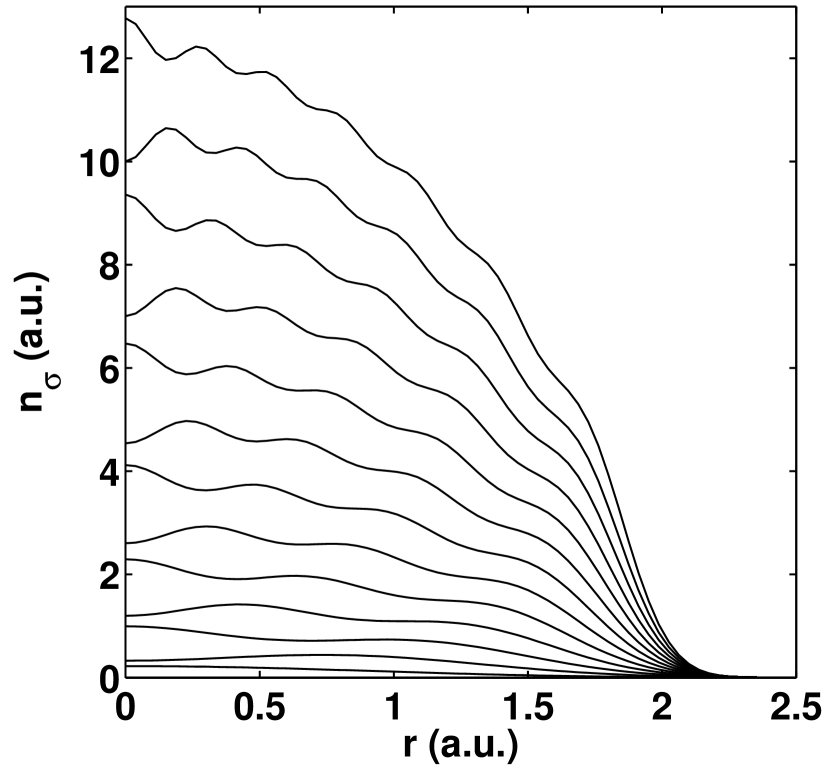
Figure 1: Electron densities for parabolic quantum dots with $N=2,\ldots,182$ electrons scaled according to Eq. (13). As a function of $N$ (from bottom to top), the spatial extent is preserved and the relative density oscillations become smaller.

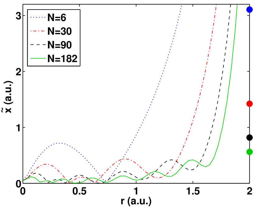
Figure 2: Dimensionless gradient ${\tilde{x}}$ for (scaled) parabolic quantum dots with $N=6,\,30,\,90,\,182$, respectively (cf. the densities in 1). The circles on the right correspond to the mean values of $x$ in the range $r=0\ldots 2$ a.u.

The density satisfies asymptotically the scaling relation

$$n_{{\rm TF},N}({\bf r})=Nn_{{\rm TF},1}({\bf r})\;.$$ (14)

Using Eq. (14) in Eqs. (3) and (11) we find that the LDA exchange energies are of the order $N^{4/3}$, and the second-order gradient corrections are of the order $N^{1/2}$, respectively. 3 shows that the LDA and exact exchange (EXX) energies, the latter evaluated within the Krieger-Lee-Iafrate ³¹ (KLI) approximation, converge to the same value at the order $N^{4/3}$. This analysis justifies using the value $C^{\rm 2D}_{\rm X}=-16/(3\sqrt{\pi})$ that stems from the 2D-LDA.

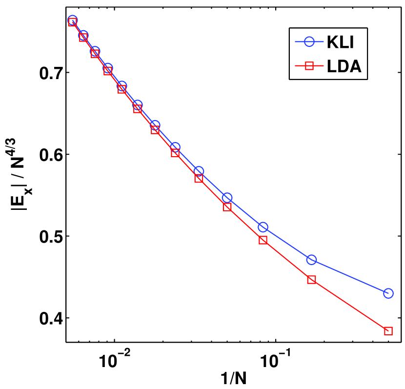
Figure 3: Comparison of exchange energies of the exact-exchange scheme in the KLI approximation and the two-dimensional local-density approximation (LDA) for a set of parabolic quantum dots at the order of $N^{4/3}$ (see text). The LDA results approach the KLI values as a function of $N$.

Now we proceed to the next order, $N^{1/2}$, and try to determine $\beta_{\rm 2D}$ numerically. 4 shows the relative error of the 2D-B88 functional as a function of $\beta_{\rm 2D}$ for the same set of parabolic quantum dots with $N=2,6,12,\ldots,182$. For each $N$, we determine the optimal $\beta_{\rm 2D}$ that gives zero error. The inset of 4 shows the behavior of this sequence. A simple polynomial fit leads to $\beta_{\rm 2D}=0.007$ in the $N\rightarrow\infty$ limit. We point out, however, that there is uncertainty in this value beacause of the following reasons. First, our analysis is limited by $N_{\rm max}=182$ due to the demanding convergence of the EXX-KLI reference results on a cartesian grid. This prevents us to fully explore the asymptotic region, and we cannot exclude the possibility of small numerical errors at the order of $N^{4/3}$ affecting the estimation made at next (lower) order in $N$. Secondly, the full optimized-effective-potential (OEP) scheme might lead to a different optimal value of $\beta_{\rm 2D}$, although it is known (in the 3D case) that the KLI approximation is typically very close to the OEP result. Thirdly, different confinement/boundary conditions (i.e., different types of turning points) can, in principle, lead to different (yet fully non-empirical) optimal values for $\beta_{\rm 2D}$. Therefore, having a different reference system instead of a parabolic quantum dot could affect the result as well; this aspect is touched in the next section, where we explore the performance of our functional on quantum rings.

Despite the uncertainties listed above, the general principles in the determination of $\beta_{\rm 2D}$ are clear. Therefore we proceed by choosing $\beta_{\rm 2D}=0.007$, and assess the performance of the functional in detail in the following section.

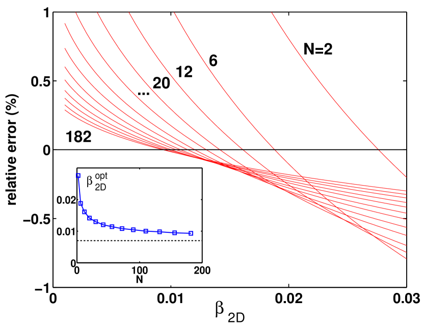
Figure 4: Relative error of the 2D-B88 functional with respect to the EXX-KLI results (see text) as a function of $\beta_{\rm 2D}$ for parabolic quantum dots with $N=2,\ldots,182$. The optimal $\beta_{\rm 2D}$ (zero error) as a function of $N$ are seen to converge in the inset. The horizontal line in the inset shows our choice $\beta_{\rm 2D}\rightarrow 0.007$.

3 Performance in applications

Next we test our 2D-B88 functional self-consistently for realistic 2D systems in comparison with exchange-only energies obtained with the KLI and local-density approximations. We shall take a look at systems not included in the estimation of $\beta_{\rm 2D}$. 1 shows the exchange energies of parabolic QDs with various $N$ and confinement strengths $\omega$ [see Eq. (12)]. The relative errors of the approximations are given in the last two columns. Overall, we find excellent agreement between 2D-B88 and EXX-KLI with a mean relative error of $1.7\%$ for the whole set. In comparison, the 2D-LDA yields a mean error of $5.2\%$. We note that, as expected, both approximations improve their accuracy as a function of $N$.

Table 1: Exchange energies (in atomic units) for parabolic quantum dots with varying $N$ and confinement strength $\omega$. The columns correspond to the exact exchange in the KLI approximation, the local density-approximation (LDA), and the generalized-gradient approximation presented in this work (2D-B88).

$N$	$\omega$	$-E^{\rm KLI}_{\rm x}$	$-E_{\rm x}^{\rm LDA}$	$-E_{\rm x}^{\rm 2D-B88}$	$|\Delta_{\rm rel}^{\rm LDA}|$	$|\Delta_{\rm rel}^{\rm 2D-B88}|$
2	0.5	0.7291	0.6495	0.6992	10.9$\%$	4.10$\%$
2	1.5	1.3583	1.2147	1.3048	10.6$\%$	3.94$\%$
2	2.5	1.7979	1.6106	1.7284	10.4$\%$	3.87$\%$
2	3.5	2.1571	1.9343	2.0745	10.3$\%$	3.83$\%$
6	0.5	2.4707	2.3392	2.4311	5.32$\%$	1.60$\%$
6	1.5	4.7267	4.4823	4.6486	5.17$\%$	1.65$\%$
6	2.5	6.3311	6.0081	6.2266	5.10$\%$	1.65$\%$
6	3.5	7.6509	7.2638	7.5252	5.06$\%$	1.64$\%$
12	0.5	5.4316	5.2571	5.3875	3.21$\%$	0.81$\%$
12	1.5	10.535	10.206	10.444	3.13$\%$	0.87$\%$
12	2.5	14.204	13.765	14.080	3.09$\%$	0.88$\%$
12	3.5	17.237	16.709	17.086	3.06$\%$	0.88$\%$
20	0.5	9.7651	9.5537	9.7229	2.16$\%$	0.43$\%$
20	1.5	19.107	18.704	19.013	2.11$\%$	0.49$\%$
20	2.5	25.874	25.334	25.744	2.09$\%$	0.50$\%$
20	3.5	31.490	30.837	31.330	2.07$\%$	0.51$\%$
mean error					5.2$\%$	1.7$\%$

In 2 we examine the performance of the 2D-B88 in QDs at low electron densities (small confinement strengths for only a few electrons). This regime is important in view of QD applications exploiting strongly correlated electrons. Again, we find that 2D-B88 clearly overperforms the LDA and yields very accurate exchange energies in comparison with the EXX-KLI. However, it remains to be tested how the 2D-B88 works in combination with a carefully chosen functional for the correlation. Only such a combined functional would be truly useful for applications in the low-density regime.

3 shows exchange energies for fully spin-polarized ($S=N/2$) parabolic quantum dots with a relatively low confinement strength. As in the previous examples, 2D-B88 is very accurate. This test validates the usability of the functional in a fully spin-dependent fashion according to the above formulation.

Table 2: Exchange energies (in atomic units) for low-density parabolic quantum dots. The columns correspond to the exact exchange in the KLI approximation, the local density-approximation (LDA), and the generalized-gradient approximation presented in this work (2D-B88).

$N$	$\omega$	$-E^{\rm KLI}_{\rm x}$	$-E_{\rm x}^{\rm LDA}$	$-E_{\rm x}^{\rm 2D-B88}$	$|\Delta_{\rm rel}^{\rm LDA}|$	$|\Delta_{\rm rel}^{\rm 2D-B88}|$
2	1	1.0831	0.9673	1.0398	10.7$\%$	4.00$\%$
2	1/4	0.4851	0.4312	0.4647	11.1$\%$	4.21$\%$
2	1/6	0.3801	0.3376	0.3640	11.2$\%$	4.24$\%$
2	1/16	0.2075	0.1844	0.1993	11.1$\%$	3.95$\%$
2	1/36	0.1275	0.1141	0.1268	10.5$\%$	0.55$\%$
6	1/4	1.6185	1.5312	1.5943	5.39$\%$	1.50$\%$
6	1/16	0.6766	0.6403	0.6697	5.37$\%$	1.02$\%$
mean error					9.3$\%$	2.8$\%$

Table 3: Exchange energies (in atomic units) for spin-polarized ($S=N/2$) parabolic quantum dots. The columns correspond to the exact exchange in the KLI approximation, the local density-approximation (LDA), and the generalized-gradient approximation presented in this work (2D-B88).

$N$	$\omega$	$-E^{\rm KLI}_{\rm x}$	$-E_{\rm x}^{\rm LDA}$	$-E_{\rm x}^{\rm 2D-B88}$	$|\Delta_{\rm rel}^{\rm LDA}|$	$|\Delta_{\rm rel}^{\rm 2D-B88}|$
2	1/4	0.6645	0.6018	0.6421	9.43$\%$	3.37$\%$
3	1/4	1.0146	0.9533	0.9987	6.04$\%$	1.57$\%$
4	1/4	1.4303	1.3363	1.4019	6.57$\%$	1.99$\%$
5	1/4	1.8091	1.7228	1.7876	4.77$\%$	1.19$\%$
6	1/4	2.1973	2.1177	2.1813	3.62$\%$	0.73$\%$
2	1/16	0.3182	0.2765	0.3035	13.1$\%$	4.62$\%$
3	1/16	0.4607	0.4296	0.4631	6.75$\%$	0.52$\%$
4	1/16	0.6697	0.5979	0.6487	10.7$\%$	3.14$\%$
5	1/16	0.8165	0.7607	0.8064	6.83$\%$	1.24$\%$
6	1/16	0.9709	0.9265	0.9853	4.57$\%$	1.48$\%$
mean error					7.2%	2.0%

Besides the exchange energies, it is informative to compare the exchange-hole potentials as well as the Kohn-Sham exchange potentials. 5(a) shows $U_{{\rm X},\sigma}$ for an $N=20$ parabolic QD with $\omega=0.4217$ a.u. The structure of the potential in the central part (within the shells) is very similar in the LDA and 2D-B88. However, the latter functional is able to describe the asymptotic behavior very accurately in comparison with the EXX-KLI result. In turn, this leads to accurate exchange energies given by 2D-B88. The behavior at large $r$ is expected due to the form in Eq. (4) that resembles the asymptotically corrected functional for the exchange-correlation potential in Ref. ³².

The Kohn-Sham exchange potentials $V_{\rm X}$ are shown in 5(b). In this case, neither LDA nor 2D-B88 are able to give the correct asymptotic behavior. However, it is interesting to see that the 2D-B88 potential produces the shell structure more accurately than the LDA at $0<r\lesssim 5$ a.u. We also find close similarity in the shell region between the 2D-B88 and the meta-GGA result suggested in Ref. ²⁴ for $V_{\rm X}$. We note, however, that the values in the lower panel of Fig. 4 in that reference miss a factor of two.

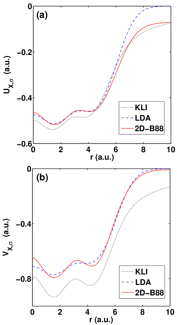
Figure 5: Self-consistent exchange-hole potentials (a) and Kohn-Sham exchange potentials (b) calculated with EXX-KLI, 2D-LDA, and 2D-B88, respectively (exchange only) for a 20-electron parabolic quantum dot with $\omega=0.4217$ a.u.

Table 4: Exchange energies (in atomic units) for a quantum ring (see text). The columns correspond to the exact exchange in the KLI approximation, the local density-approximation (LDA), and the generalized-gradient approximation presented in this work (2D-B88).

$N$	$-E^{\rm KLI}_{\rm x}$	$-E_{\rm x}^{\rm LDA}$	$-E_{\rm x}^{\rm 2D-B88}$	$|\Delta_{\rm rel}^{\rm LDA}|$	$|\Delta_{\rm rel}^{\rm 2D-B88}|$
6	2.1590	2.1095	2.2668	2.29$\%$	4.99$\%$
10	4.5192	4.3106	4.5458	4.62$\%$	0.59$\%$
14	7.1495	6.7915	7.0867	5.01$\%$	0.88$\%$
20	10.820	10.568	10.883	2.33$\%$	0.58$\%$
24	13.356	13.126	13.437	1.72$\%$	0.61$\%$
mean error				3.2%	1.5%

For the usefulness of the 2D-B88 functional it is important to test its validity for different physical systems. In the following we open the discussion to this direction by examining a quantum ring. As the system has a different topology from a QD it gives useful insights into the general applicability of the functional. The external potential is now defined as $V_{\rm ext}(r)=\omega^{2}(r-r_{0})^{2}/2$, where we set $\omega=1$ a.u. and $r_{0}=3$ a.u. The results for exchange energies are given in 4. Overall, 2D-B88 yields significantly more accurate results than the LDA except for the $N=6$ ring. In that particular case the width of the electron density along the perimeter is relatively small – approaching the quasi-one-dimensional system, which calls for more elaborate ways to deal with the electronic exchange. ¹⁶ Nevertheless, at $N>6$ the accuracy of the 2D-B88 is excellent: the deviation from the KLI exchange energy remains below $1\%$.

4 Summary

In this work we constructed a generalized-gradient approximation for the exchange energy in two dimensions (2D). With the construction we overcame the known problems in finding finite coefficients for the 2D gradient expansion through, e.g., the Kirzhnits expansion. Our formulation follows the B88 exchange functional. The final coefficient was then found through a fitting to properly scaled 2D harmonic oscillators in the large-$N$ limit, corresponding to the high-Z limit in three-dimensional atomic systems. We tested the obtained exchange-energy functional for various quantum dots and found excellent agreement with exact-exchange results and a significant improvement over the standard local-density approximation. The functional also leads to a proper asymptotic tail of the exchange-hole potential and a more accurate exchange potential than that of the local-density approximation. The generality of the functional was confirmed in tests for low-density quantum dots, spin-polarized systems, as well as 2D quantum rings. Possible further extensions of the present construction could include adaptation to the recently developed density-functional formalism for strongly interacting electrons. ^{33, 34}

We thank Alexander Odriazola for numerical support and useful discussions. The work was supported by the European Community s FP7 through the CRONOS project, grant agreement no. 280879, the Academy of Finland through project no. 126205, and COST Action CM1204 XLIC. S.P. also acknowledges support from NSF Grant CHE-1112442 and discussions with Kieron Burke. J.G.V. acknowledges support from the FCT Grant No.SFRH/BD/38340/2007.

References

- 1 S. M. Reimann and M. Manninen. Rev. Mod. Phys. 2002, 74, 1283 ; L. P. Kouwenhoven, D. G. Austing and S. Tarucha. Rep. Prog. Phys. 2001, 64, 701.
- 2 For review, see M. Polini, F. Guinea, M. Lewenstein, H.C. Manoharan, and V. Pellegrini. Nat. Nanotechnol. 2013 , 8, 625.
- 3 U. von Barth. Phys. Scripta 2004 , T109,9 .
- 4 Density Functional Theory ; R. M. Dreizler and E. K. U. Gross; Springer: Berlin, 1990.
- 5 A Primer in Density Functional Theory; C. Fiolhais, F. Nogueira, and M. A. L. Marques, Eds.; Springer-Verlag: Berlin, 2003.
- 6 J. P. Perdew and S. Kurth; Density Functionals for Non-relativistic Coulomb Systems in the New Century. In A Primer in Density Functional Theory, first edition; C. Fiolhais, F. Nogueira, and M. A. L. Marques, Eds.; Springer-Verlag: Berlin, 2003; pp 1. G. E. Scuseria and V. N. Staroverov; Progress in the development of exchange-correlation functionals. In Theory and Applications of Computational Chemistry: The First Forty Years, first edition; C. E. Dykstra, G. Frenking, K. S. Kim, and G. E. Scuseria, Eds.; Elsevier: Amsterdam, 2005; pp. 669.
- 7 Y.-H. Kim, I.-H. Lee, S. Nagaraja, J.-P. Leburton, R. Q. Hood, and R. M. Martin. Phys. Rev. B 2000 , 61, 5202.
- 8 L. Pollack and J. P. Perdew. J. Phys.: Condens. Matt. 2000 , 12, 1239.
- 9 L. Chiodo, L. A. Constantin, E. Fabiano, and F. Della Sala. Phys. Rev. Lett. 2012 , 108, 126402.
- 10 A. K. Rajagopal and J. C. Kimball. Phys. Rev. B 1977 , 15, 2819.
- 11 B. Tanatar and D. M. Ceperley. Phys. Rev. B 1989 , 39, 5005.
- 12 C. Attaccalite, S. Moroni, P. Gori-Giorgi, and G. B. Bachelet. Phys. Rev. Lett. 2002 , 88, 256601.
- 13 S. Pittalis, E. Räsänen, N. Helbig, and E. K. U. Gross. Phys. Rev. B 2007 , 76, 235314.
- 14 S. Pittalis, E. Räsänen, J. G. Vilhena, and M. A. L. Marques. Phys. Rev. A 2009 , 79, 012503.
- 15 S. Pittalis, E. Räsänen, C. Proetto, and E. K. U. Gross. Phys. Rev. B 2009 , 79, 085316.
- 16 E. Räsänen, S. Pittalis, C. R. Proetto, and E. K. U. Gross. Phys. Rev. B 2009 , 79, 121305(R).
- 17 S. Pittalis, E. Räsänen, and E. K. U. Gross. Phys. Rev. A 2009 , 80, 032515.
- 18 S. Pittalis and E. Räsänen. Phys. Rev. B 2010 , 82, 165123.
- 19 A. Putaja, E. Räsänen, R. van Leeuwen, J. G. Vilhena, and M. A. L. Marques. Phys. Rev. B 2012 , 85, 165101.
- 20 P. Elliot and K. Burke. Can. J. Chemistry 2009 , 87, 1485.
- 21 A.D. Becke. Phys. Rev. A 1988 , 38, 3098.
- 22 J. Schwinger. Phys. Rev. A 1981 , 24, 2353.
- 23 C.L. Fefferman and C.L. Seco. B. Am. Math. Soc. 1990 , 23, 525.
- 24 S. Pittalis, E. Räsänen, and C. R. Proetto. Phys. Rev. B 2010 , 81, 115108.
- 25 A. D. Becke. J. Chem. Phys. 1993 , 98, 5648; C. Lee, W. Yang, and R. G. Parr. Phys. Rev. B 1988 , 37, 785; P. Stephens, F. Devlin, C. Chabalowski, and M. Frisch. J. Phys. Chem. 1994 , 98, 11623.
- 26 J. P. Perdew, A. Ruzsinszky, G. I. Csonka, O. A. Vydrov, G. E. Scuseria, L. A. Constantin, X. Zhou, and K. Burke. Phys. Rev. Lett. 2008 , 100, 136406; 2009 , 102, 039902(E).
- 27 E. Lieb and B. Simon. Phys. Rev. Lett. 1973 , 31, 681.
- 28 E. Lieb and B. Simon. Adv. Math. 1977 , 23, 22.
- 29 E. H. Lieb, J. P. Solovej, and J. Yngvason. Phys. Rev. B 1995 , 51, 10646.
- 30 M. A. L. Marques, A. Castro, G. F. Bertsch, and A. Rubio. Comput. Phys. Commun. 2003 , 151, 60; A. Castro, H. Appel, M. Oliveira, C. A. Rozzi, X. Andrade, F. Lorenzen, M. A. L. Marques, E. K. U. Gross, and A. Rubio. Phys. Status Solidi B 2006 , 243, 2465.
- 31 J. B. Krieger, Y. Li, and G. J. Iafrate. Phys. Rev. A 1992 , 45, 101.
- 32 S. Pittalis and E. Räsänen. Phys. Rev. B 2010 , 82, 195124.
- 33 P. Gori-Giorgi, M. Seidl, and G. Vignale. Phys. Rev. Lett. 2009 , 103, 166402.
- 34 C. B. Mendl, F. Malet, and P. Gori-Giorgi. Phys. Rev. B 2014 , 89, 125106.