“TNOs are Cool”: A survey of the trans-Neptunian region

Abstract

Context. The Kuiper belt is formed of planetesimals which failed to grow to planets and its dynamical structure has been affected by Neptune. The classical Kuiper belt contains objects both from a low-inclination, presumably primordial, distribution and from a high-inclination dynamically excited population.

Aims. Based on a sample of classical TNOs with observations at thermal wavelengths we determine radiometric sizes, geometric albedos and thermal beaming factors for each object as well as study sample properties of dynamically hot and cold classicals.

Methods. Observations near the thermal peak of TNOs using infra-red space telescopes are combined with optical magnitudes using the radiometric technique with near-Earth asteroid thermal model (NEATM). We have determined three-band flux densities from Herschel/PACS observations at 70.0, 100.0 and $160.0\ \mathrm{\mu m}$ and Spitzer/MIPS at 23.68 and $71.42\ \mathrm{\mu m}$ when available. We use reexamined absolute visual magnitudes from the literature and ground based programs in support of Herschel observations.

Results. We have analysed 18 classical TNOs with previously unpublished data and re-analysed previously published targets with updated data reduction to determine their sizes and geometric albedos as well as beaming factors when data quality allows. We have combined these samples with classical TNOs with radiometric results in the literature for the analysis of sample properties of a total of 44 objects. We find a median geometric albedo for cold classical TNOs of $0.14_{-0.07}^{+0.09}$ and for dynamically hot classical TNOs, excluding the Haumea family and dwarf planets, $0.085_{-0.045}^{+0.084}$. We have determined the bulk densities of Borasisi-Pabu ($2.1_{-1.2}^{+2.6}$ g cm^-3), Varda-Ilmarë ($1.25_{-0.43}^{+0.40}$ g cm^-3) and 2001 QC₂₉₈ ($1.14_{-0.30}^{+0.34}$ g cm^-3) as well as updated previous density estimates of four targets. We have determined the slope parameter of the debiased cumulative size distribution of dynamically hot classical TNOs as $q$=2.3$\pm$0.1 in the diameter range 100$<$$D$$<$500 km. For dynamically cold classical TNOs we determine $q$=5.1$\pm$1.1 in the diameter range 160$<$$D$$<$280 km as the cold classical TNOs have a smaller maximum size.

1 Introduction

Transneptunian objects (TNO) are believed, based on theoretical modeling, to represent the leftovers from the formation process of the solar system. Different classes of objects may probe different regions of the protoplanetary disk and provide clues of different ways of accretion in those regions (Morbidelli et al., (2008)). Basic physical properties of TNOs, such as size and albedo, have been challenging to measure. Only a few brightest TNOs have size estimates using direct optical imaging (e.g. Quaoar with Hubble; (Brown and Trujillo, , 2004)). Stellar occultations by TNOs provide a possibility to obtain an accurate size estimate, but these events are rare and require a global network of observers (e.g. Pluto’s moon Charon by Sicardy et al., (2006); and a member of the dynamical class of classical TNOs, 2002 TX₃₀₀, by Elliot et al. , 2010). Predictions of occultations are limited by astrometric uncertainties of both TNOs and stars. Combining observations of reflected light at optical wavelengths with thermal emission data, which for TNOs peaks in the far-infrared wavelengths, allows us to determine both size and geometric albedo for large samples of targets. This radiometric method using space-based ISO (e.g. Thomas et al., (2000)), Spitzer (e.g. (Stansberry et al., , 2008), (Brucker et al., , 2009)) and Herschel data ((Müller et al., , 2010), (Lellouch et al., , 2010), (Lim et al., , 2010), (Santos-Sanz et al., , 2012), (Mommert et al., , 2012), (Vilenius et al., , 2012), Pál et al., (2012), (Fornasier et al., , 2013)) has already changed the size estimates of several TNOs compared to those obtained by using an assumed albedo and has revealed a large scatter in albedos and differences between dynamical classes of TNOs.

Observations at thermal wavelengths also provide information about thermal properties ((Lellouch et al., , 2013)). Depending on the thermal or thermophysical model selected it is possible to derive the thermal beaming factor or the thermal inertia, and constrain other surface properties. Ground-based submillimeter observations can also be used to determine TNO sizes using the radiometric method (e.g. Jewitt et al., (2001)), but this technique has been limited to very few targets so far.

TNOs, also known as Kuiper belt objects (KBO), have diverse dynamical properties and they are divided into classes. Slightly different definitions and names for these classes are available in the literature. Classical TNOs (hereafter CKBO) reside mostly beyond Neptune on orbits which are not very eccentric and not in mean motion resonance with Neptune. We use the Gladman et al. (2008) classification: CKBOs are non-resonant TNOs which do not belong to any other TNO class. The eccentricity limit is $e$ $\lesssim$ $0.24$, beyond which objects belong to detached objects or scattering/scattered objects. Classical TNOs with semimajor axis $39.4$ $<$ $a$ $<$ $48.4\ \mathrm{AU}$ occupy the main classical belt, whereas inner and outer classicals exist at smaller and larger semi-major axis, respectively. Apart from the Gladman system, another common classification is defined by the Deep Eplictic Survey Team (DES, Elliot et al. 2005). For the work presented here, the most notable difference between the two systems is noticed with high-inclination objects. Many of them are not CKBOs in the DES system.

In the inclination/eccentricity space CKBOs show two different populations, which have different frequency of binary systems (Noll et al., (2008)), different luminosity functions (LF; Fraser et al. 2010), different average geometric albedos (Grundy et al., (2005); Brucker et al. 2009) and different color distributions ((Peixinho et al., , 2008)). The low-inclination “cold” classicals are limited to the main classical belt and have a higher average albedo, more binaries and a steeper LF-derived size distribution than high-inclination “hot” classicals. Some amount of transfer between the hot and cold CKBOs is possible with an estimated maximum of 5% of targets in either population originating from the other than its current location (Volk and Malhotra, (2011)).

The “TNOs are Cool”: A survey of the trans-Neptunian region open time key program (Müller et al., (2009)) of Herschel Space Observatory has observed 12 cold CKBOs, 29 hot CKBOs, and five CKBOs in the inner classical belt, which are considered to be dynamically hot. In addition, eight CKBOs have been observed only by Spitzer Space Telescope, whose TNO sample was mostly overlapping with the Herschel one.

This paper is organized in the following way. We begin by describing our target sample in Section 2.1, followed by Herschel observations and their planning in Section 2.2 and Herschel data reduction in Section 2.3. More far-infrared data by Spitzer are presented in Section 2.4 and absolute visual magnitudes in Section 2.5. Thermal modeling combining the above mentioned data is described in Section 3.1 and the results for targets in our sample in Section 3.2, comparing them with earlier results when available (Section 3.3). In Section 4 we discuss sample properties, cumulative size distributions, correlations and binaries as well as debiasing of the measured size distributions. Conclusions of the sample analysis are given in Section 5.

2 Target sample and observations

2.1 Target sample

The classification of targets in the “TNOs are Cool” program within the Gladman et al. (2008) framework is based on the list used by Minor Bodies in the Outer Solar System 2 data base (MBOSS-2, Hainaut et al. 2012 and C. Ejeta, priv. comm.). The inclination distributions of the dynamically cold and hot components of CKBOs are partly overlapping. A cut-off limit of $i$ $=$ $4.5\degr$ is used in this work, and the inclinations we use from the Minor Planet Center are measured with respect to the ecliptic plane, which deviates slightly from the invariable plane of the Solar System, or the average Kuiper belt plane. All the cold CKBOs with measured sizes available have inclinations $i$$<$4.0$\degr$ (see Table 6 in Section 4). Three CKBOs listed as dynamically hot in Table 7 (2000 OK₆₇, 2001 QD₂₉₈ and Altjira) have 4.5$<$$i$$<$5.5$\degr$. Since the two populations overlap in the inclination space some targets close to the cut-off limit could belong to the other population. In the DES classification system all targets in Table 1 with $i$ $>$ $15\degr$ would belong to the scattered-extended class of TNOs. DES uses the Tisserand parameter and orbital elements in the CKBO/scattered objects distinction, whereas the Gladman system requires an object to be heavily interacting with Neptune in order to be classified as a scattered object.

In this work we have reduced the flux densities of 16 CKBOs observed with Herschel. Together with Vilenius et al. (2012), Fornasier et al. (2013) and Lellouch et al. (2013) this work completes the set of CKBOs observed by Herschel, except for the classical Haumea family members with water signatures in their spectra, whose properties differ from the “bulk” of CKBOs (Stansberry et al., in prep.). Photometric 3-band observations were done in 2010-2011 with Herschel/PACS in the wavelength range 60–$210\ \mathrm{\mu m}$. Seven of the 16 targets have been observed also with two bands of Spitzer/MIPS imaging photometer at 22–$80\ \mathrm{\mu m}$ in 2004-2008. In addition, our target sample (Table 1) includes two previously unpublished targets 2003 QR₉₁ and 2001 QC₂₉₈ observed only with MIPS and are included in the radiometric analysis of this work.

The relative amount of binaries among the cold CKBOs with radiometric measurements is high (Table 6) with only very few non-binaries. While the binary fraction among cold CKBOs has been estimated to be 29% (Noll et al., (2008)) the actual frequency may be higher because there probably are binaries which have not been resolved with current observing capabilities. Furthermore, in the target selection process of ”TNOs are Cool” we aimed to have a significant sample of binary TNOs observed, and the highest binary fraction of all dynamical classes is in the cold sub-population of CKBOs.

For sample analysis we have included all CKBOs with radiometric results from this work and literature, some of which have been reanalyzed in this work. We achieve a total sample size of 44 targets detected with either Herschel or Spitzer (Tables 6 and 7). The absolute V-magnitudes ($H_{\mathrm{V}}$, see Section 2.5) of the combined sample range from about 3.5 to 8.0 mag (0.1-8.0 mag if dwarf planets are included). A typical characteristic of CKBOs is that bright classicals have systematically higher inclinations than fainter ones (Levison and Stern 2001). Our combined sample shows a moderate correlation (see Section 4.5.2) between absolute magnitude and inclination at 4$\sigma$ level of significance. For about half of the targets a color taxonomy is available. Almost all very red targets (RR) in the combined sample are at inclinations $i$ $<$ $12\degr$. This is consistent with Peixinho et al. (2008) who report a color break at $i$ $=$ $12\degr$ instead of at the cold/hot boundary inclination near 5$\degr$.

Table 1: Orbital and color properties of the sample of 18 classical TNOs with new flux densities presented in this work.

Target		$q$	$Q$	$i$	$e$	$a$	Color	Spectral slope	V-R
		(AU)	(AU)	(°)			taxa	(% / 100 nm)
(2001 QS$_322$)		42.3	46.1	0.2	0.043	44.2	…	…	…
66652 Borasisi (1999 RZ$_253$)	B	40.0	47.8	0.6	0.088	43.9	RR	$33.8\pm 2.7$	$0.646\pm 0.058$
(2003 GH$_55$)		40.6	47.3	1.1	0.076	44.0	…	$26.0\pm 5.6$	$0.63\pm 0.06$
135182 (2001 QT$_322$) in inner belt		36.6	37.9	1.8	0.018	37.2	…	$15.6\pm 11.1$	$0.53\pm 0.12$
(2003 QA$_91$)	B	41.4	47.7	2.4	0.071	44.5	…	…	…
(2003 QR$_91$)	B	38.1	55.0	3.5	0.182	46.6	…	…	…
(2003 WU$_188$)	B	42.4	46.3	3.8	0.043	44.3	…	…	…
35671 (1998 SN$_165$) in inner belt		36.4	39.8	4.6	0.045	38.1	BB	$6.9\pm 3.1$	$0.444\pm 0.078$
(2001 QD$_298$)		40.3	45.1	5.0	0.056	42.7	…	$30.4\pm 8.3$	$0.67\pm 0.09$
174567 Varda (2003 MW$_12$)	B	39.0	52.2	21.5	0.144	45.6	IR	$19.2\pm 0.6$	…
86177 (1999 RY$_215$)		34.5	56.5	22.2	0.241	45.5	BR	$3.8\pm 3.5$	$0.358\pm 0.090$
55565 (2002 AW$_197$)		41.2	53.2	24.4	0.127	47.2	IR	$22.1\pm 1.4$	$0.602\pm 0.031$
202421 (2005 UQ$_513$)		37.3	49.8	25.7	0.143	43.5	…	$18.1\pm 2.0$	…
(2004 PT$_107$)		38.2	43.1	26.1	0.060	40.6	…	…	$0.65\pm 0.10$
(2002 GH$_32$)		38.1	45.7	26.7	0.091	41.9	…	$24.8\pm 4.7$	$0.425\pm 0.228$
(2001 QC$_298$)	B	40.6	52.1	30.6	0.124	46.3	…	$10.3\pm 2.4$	$0.490\pm 0.030$
(2004 NT$_33$)		37.0	50.1	31.2	0.150	43.5	BB-BR	…	…
230965 (2004 XA$_192$)		35.5	59.4	38.1	0.252	47.4	…	…	…

2.2 Herschel observations

Herschel Space Observatory (Pilbratt et al., (2010)) was orbiting the Lagrange 2 point of the Earth-Sun system in 2009-2013. It has a 3.5 m radiatively cooled telescope and three science instruments inside a superfluid helium cryostat. The photometer part of the PACS instrument (Poglitsch et al., (2010)) has a rectangular field of view of $1.75\arcmin$ $\times$ $3.5\arcmin$. It has two bolometer arrays, the short-wavelength one is for wavelengths 60 – $85\ \mathrm{\mu m}$ or 85 – $125\ \mathrm{\mu m}$, selectable by a filter wheel, and the long-wavelength array for 125 – $210\ \mathrm{\mu m}$. The absolute calibration 1-$\sigma$ uncertainty is 5% in all bands (Balog et al. (2013)). The detector pixel sizes are $3.2\arcsec\times 3.2\arcsec$ in the short-wavelength array, whereas the long-wavelength array has larger pixels of $6.4\arcsec\times 6.4\arcsec$. The instrument is continuously sampling the detectors and produces 40 frames/s, which are averaged on-board by a factor of four. Herschel recommended to use the scanning technique for point sources instead of chopping and nodding, to achieve better sensitivity (PACS AOT release note (2010)). Pixels in the image frames, sampled continuously while the telescope was scanning, were mapped in the data reduction pipeline (see Section 2.3) into pixels of a sub-sampled output image.

Our observations (Table 2) with PACS followed the same strategy as in Vilenius et al. (2012). We made three-band observations of all targets in two scan directions of the rectangular array, and repeated the same observing sequence on a second visit. We used mini-scan maps with 2-6 repetitions per observation. The final maps are combinations of four observations/target, except at the $160\ \mathrm{\mu m}$ band where all eight observations/target were available independent of the filter wheel selection. To choose the number of repetitions, i.e. the duration of observations, we used a thermal model (see Section 3.1) to predict flux densities. We adopted a default geometric albedo of 0.08 and a beaming factor of 1.25 for observation planning purposes. For two bright targets we used other values based on earlier Spitzer results ((Stansberry et al., , 2008)): for 1998 SN₁₆₅ a lower geometric albedo of 0.04 and for 2002 AW₁₉₇ a higher geometric albedo of 0.12. In the combined maps the predicted instrumental signal-to-noise ratios (SNR) for the 16 targets with the above assumptions were SNR$\sim$ 13 (faintest target SNR$\sim$ 4) at the 70 and $100\ \mathrm{\mu m}$ channels and SNR$\sim$ 7 (faintest target SNR$\sim$ 2) at the $160\ \mathrm{\mu m}$ channel. The sensitivity of the $70\ \mathrm{\mu m}$ channel is usually limited by instrumental noise, while the aim of our combination of observations is to remove the background confusion noise affecting the other two channels, most notably the $160\ \mathrm{\mu m}$ band.

The selection of the observing window was optimized to utilize the lowest far-infrared confusion noise circumstances (Kiss et al., (2005)) of each target during the Herschel mission. Targets were visited twice within the same observing window with a similar set of 2x2 observations on each of the two visits for the purpose of background subtraction (Kiss et al., (2013)). The time gap between the visits was 11-42 hours depending on the proper motion of the target.

2.3 PACS Data reduction

We used data reduction and image combination techniques developed within the “TNOs are Cool” key program (Kiss et al., (2013) and references cited therein). Herschel Interactive Processing Environment (HIPE, version 9.0 / CIB 2974) was used to produce Level 2 maps with modified scan map pipeline scripts. The pipeline script provided a two-stage high-pass filtering procedure to handle the 1/f noise, which is dominating the timelines of individual detectors in the PACS photometer arrays. The script removes from each timeline, excluding the masked parts of timelines where we expect the source to be present, a value obtained by a running median filter. The filter width parameters we used were typically 8/9/16 readouts, and for some targets 10/15/25 readouts at the 70/100/$160\ \mathrm{\mu m}$ channels, respectively. We set the map-pixel sizes to 1.1″/pixel, 1.4″/pixel and 2.1″/pixel for the three channels, respectively, to properly sample the point spread functions.

For combining the projected output images and reducing the background we use two methods: “super-sky-subtracted” images ((Brucker et al., , 2009), (Santos-Sanz et al., , 2012)) and “double-differential” images ((Mommert et al., , 2012), Kiss et al., (2013)). The “super-sky” is constructed by masking the source (or an area surrounding the image center when the target is too faint to be recognized in individual images) in each individual image, combining these sky images and subtracting this combined background from each individual image. Then, all background-subtracted images are co-added in the co-moving frame of the target. The “double-differential” images are produced in a different way. Since the observing strategy has been to make two sets of observations with similar settings, we subtract the combined images of the two visits. This yields a positive and a negative beam of the moving source with background structures eliminated. A duplicate of this image is shifted to match the positive beam of the original image with the negative one of the duplicate. After subtracting these from each other we have a double-differential image with one positive and two negative beams, where photometry is done on the central, positive beam. It can be noted that this method works well even if there is a systematic offset in target coordinates due to uncertain astrometry. A further advantage is in the detection of faint sources: they should have one positive and two negative beams in the final image (with negative beams having half the flux density of the positive one). In both methods of combining individual observations of a target we take into account the offsets and uncertainties in pointing and assigned image coordinates (Pál et al., (2012), Kiss et al., (2013)).

Photometry is performed with DAOPHOT routines (Stetson, (1987)), which are available via commonly used astronomy software tools such as HIPE, IDL and IRAF (for details how photometry is done in the “TNOs are Cool” program see (Santos-Sanz et al., , 2012)). A color correction to flux densities is needed because TNOs have a spectral energy distribution (SED) resembling a black body whereas the PACS photometric system assumes a flat SED. The correction, based on instrumental transmission and response curves available from HIPE, is typically at the level of 2% or less depending on the temperature of the TNO. The color correction is fine-tuned in an iterative way (for details see (Vilenius et al., , 2012)). For uncertainty estimation of the derived flux density we use 200 artificial implanted sources within a region close to the source, excluding the target itself.

The color corrected flux densities from PACS are given in Table 2, where also the absolute calibration uncertainty has been included in the 1-$\sigma$ error bars. The flux densities are preferably averaged from the photometry results using the two techniques discussed above: the “super-sky-subtracted” and the “double-differential”. Since the super-sky-subtracted way gives more non-detected bands than the double-differential way we take the average only when the super-sky-subtracted method produces a 3-band detection, otherwise only flux densities based on the double-differential images are used for a given target. In Table 2 the seven targets whose flux densities at $160\,\mathrm{\mu m}$ are $>$5 mJy have flux densities averaged from the double-differential and super-sky-subtracted methods.

The flux density predictions used in the planning (Section 2.2) of these observations differ by factors of $\pm 2$ or more compared to the measured flux densities. On the average, the measured values are lower ($\sim$ 50%) than the predicted ones. Only three targets are brighter than estimated in the PACS bands and there are four targets not detected in the PACS observations. The average SNRs of detected targets are half of the average SNRs of the predictions used in observation planning.

Table 2: Herschel observations and monochromatic flux densities at all three PACS bands. 2001 QY₂₉₇ and Altjira from Vilenius et al. (2012) have been reanalysed in this work with changes in flux densities and radiometric results.

Target	1st OBSIDs	Dur.	Mid-time	$r$	$\Delta$	$\alpha$	Flux densities (mJy)
	of visit 1/2	(min)		(AU)	(AU)	(°)	$70\,\mathrm{\mu m}$	$100\,\mathrm{\mu m}$	$160\,\mathrm{\mu m}$
2001 QS322	1342212692/…2726	188.5	2011-Jan-15 22:54	42.36	42.78	1.22	$1.8\pm 1.1$	$4.0\pm 1.6$	$4.3\pm 2.0$
Borasisi	1342221733/…1806	226.1	2011-May-27 23:21	41.62	41.74	1.40	$<$1.0	$<$1.4	$<$1.4
2003 GH55	1342212652/…2714	188.5	2011-Jan-15 13:14	40.84	41.16	1.31	$2.0\pm 1.0$	$<$1.3	$<$1.4
2001 QY297	1342209492/…9650	194.8	2010-Nov-19 03:28	43.25	43.25	1.31	$<$1.3	$<$2.1	$<$2.1
2001 QT322	1342222436/…2485	226.1	2011-Jun-10 15:15	37.06	37.38	1.50	$2.6\pm 1.1$	$<$6.7	$<$1.5
2003 QA91	1342233581/…4252	226.1	2011-Dec-05 06:06	44.72	44.85	1.26	$1.8\pm 1.1$	$2.3\pm 1.3$	$<$1.6
2003 WU188	1342228922/…9040	226.1	2011-Sep-20 04:57	43.31	43.58	1.29	$<$1.0	$<$1.0	$<$1.1
1998 SN165	1342212615/…2688	113.3	2011-Jan-15 00:39	37.71	37.95	1.46	$9.5\pm 1.2$	$14.2\pm 1.9$	$5.7\pm 1.8$
2001 QD298	1342211949/…2033	188.5	2010-Dec-16 01:37	41.49	41.85	1.27	$2.7\pm 1.1$	$4.1\pm 1.3$	$<$1.3
Altjira	1342190917/…1120	152.0	2010-Feb-23 00:32	45.54	45.58	1.25	$4.5\pm 1.4$	$<$4.2	$<$2.3
Varda	1342213822/…3932	113.3	2011-Feb-08 06:52	47.62	47.99	1.11	$23.1\pm 1.7$	$26.2\pm 2.0$	$19.0\pm 2.1$
1999 RY215	1342221751/…1778	188.5	2011-May-28 01:04	35.50	35.67	1.63	$6.6\pm 1.1$	$5.7\pm 1.6$	$<$2.4
2002 AW197	1342209471/…9654	113.3	2010-Nov-19 01:59	46.34	46.27	1.24	$17.0\pm 1.3$	$20.2\pm 1.7$	$15.3\pm 1.5$
2005 UQ513	1342212680/…2722	113.3	2011-Jan-15 20:26	48.65	48.80	1.16	$5.3\pm 1.5$	$6.7\pm 2.0$	$5.6\pm 2.2$
2004 PT107	1342195396/…5462	113.3	2010-Apr-23 12:01	38.30	38.66	1.41	$8.3\pm 1.6$	$8.6\pm 2.2$	$7.9\pm 2.8$
2002 GH32	1342212648/…2710	188.5	2011-Jan-15 11:35	43.29	43.64	1.22	$<$1.1	$<$1.5	$<$1.6
2004 NT33	1342219015/…9044	113.3	2011-Apr-19 07:34	38.33	38.69	1.42	$17.3\pm 1.7$	$18.3\pm 2.0$	$9.7\pm 2.7$
2004 XA192	1342217343/…7399	75.7	2011-Mar-29 10:36	35.71	35.82	1.60	$15.0\pm 1.7$	$14.2\pm 2.2$	$8.2\pm 5.9$

2.4 Spitzer observations

The Earth-trailing Spitzer Space Telescope has a 0.85 m diameter helium-cooled telescope. The cryogenic phase of the mission ended in 2009. During that phase, one of four science instruments onboard, the Multiband Imaging Photometer for Spitzer (MIPS; Rieke et al., (2004)), provided useful photometry of TNOs at two bands: 24 and $70\ \mathrm{\mu m}$. The latter is spectrally overlapping with the PACS $70\ \mathrm{\mu m}$ band whereas the former can provide strong constraints on the temperature of the warmest regions of TNOs. The telescope-limited spatial resolution is $6\arcsec$ and $18\arcsec$ in the two bands, respectively. The nominal absolute calibration, photometric methods, and color corrections are described in Gordon et al. (2007), Engelbracht et al. (2007) and Stansberry et al. (2007). For TNOs we use larger calibration uncertainties of 3% and 6% at the 24 and $70\ \mathrm{\mu m}$ bands, respectively ((Stansberry et al., , 2008)).

Spitzer observed about 100 TNOs and Centaurs and three-quarters of them are also included in the “TNOs are Cool” Herschel program. Many of the Spitzer targets were observed multiple times within several days, with the visits timed to allow subtraction of the background. A similar technique has been applied also to the Herschel observations (Section 2.3 / “super-sky-subtraction” method). In this work and Vilenius et al. (2012) there are 20 targets (out of 35 Herschel targets analysed in these two works) which have reanalyzed Spitzer/MIPS data available (Mueller et al., in prep.). In addition, we have searched for all classical TNOs observed with Spitzer but not with Herschel: 1996 TS₆₆, 2001 CZ₃₁, 2001 QB₂₉₈, 2001 QC₂₉₈, 2002 GJ₃₂, 2002 VT₁₃₀, 2003 QR₉₁, and 2003 QY₉₀. The dynamically hot CKBOs 1996 TS₆₆ and 2002 GJ₃₂ have been published in Brucker et al. (2009), but their flux densities have been updated and reanalysed results of this work have changed their size and albedo estimates (Table 7). An updated data reduction was recently done for 2001 QB₂₉₈ and 2002 VT₁₃₀ and we use the results from Mommert (2013) for these two targets. Of the other targets only 2001 QC₂₉₈ and 2003 QR₉₁ are finally used because all the other cases do not have enough observations for a background removal or there was a problem with the observation. Spitzer flux densities used in the current work are given in Table 3. For most of these targets flux densities have been derived using multiple observations during an epoch lasting one to eight days. Borasisi was observed in two epochs in 2004 and 2008. The color corrections of CKBOs in our sample are larger than in the case of the PACS instrument. For MIPS the color corrections are 1%-10% of the flux density at $24\ \mathrm{\mu m}$ and about 10% at $70\ \mathrm{\mu m}$ obtained by a method which uses the black body temperature which fits the 24:70 flux ratio the best (Stansberry et al. , 2007).

Table 3: Spitzer/MIPS observations. Targets 2003 QR₉₁, 2001 QC₂₉₈, 1996 TS₆₆ and 2002 GJ₃₂ were not observed by Herschel. The latter two targets are from Brucker et al. (2009) and have been remodeled based on updated flux densities with significant changes in radiometric results. Flux densities of Teharonhiawako and 2001 QY₂₉₇ have been updated from those in Vilenius et al. (2012), and they have been reanalysed in this work.

Target	PID	Mid-time of observation(s)	$r$	$\Delta$	$\alpha$	MIPS $24\ \mathrm{\mu m}$ band		MIPS $70\ \mathrm{\mu m}$ band
			(AU)	(AU)	(°)	Dur. (min)	F24 (mJy)	Dur. (min)	F70 (mJy)
2001 QS322	3542	2005-Dec-03 13:12	42.32	41.87	1.23	467.2	$<0.015$	308.5	$<1.1$
Borasisi	3229	2004-Dec-02 00:29	41.16	41.16	1.41	99.1	$<0.030$	218.2	$3.6\pm 0.9$
	50024	2008-Jul-29 16:48	41.41	40.97	1.29	170.45	$0.057\pm 0.007$	369.3	$1.3\pm 0.7$
2001 QY297	50024	2008-Nov-25 02:40	43.09	42.73	1.28	170.45	$0.016\pm 0.006$	239.17	$2.0\pm 0.9$
2001 QT322	3542	2004-Dec-26 23:46	36.92	36.95	1.56	406.6	$<0.037$	406.6	$<1.5$
2003 QA91	50024	2008-Dec-28 16:34	44.91	44.87	1.29	431.8	$0.079\pm 0.006$	639.2	$3.8\pm 0.4$
Teharonhiawako	3229	2004-Nov-09 20:15	45.00	44.72	1.25	153.27	$0.027\pm 0.010$	179.03	$1.6\pm 0.6$
2003 QR91	50024	2008-Nov-24 13:26	39.12	38.70	1.37	340.9	$0.107\pm 0.007$	1074.2	$4.8\pm 0.6$
1998 SN165	55	2004-Dec-05 08:10	37.97	37.54	1.39	no observations		37.3	$<13.9$
2001 QD298	3542	2004-Nov-05 13:41	41.19	40.91	1.36	283.3	$<0.059$	283.3	$<1.5$
1996 TS66	3542	2005-Jan-29 06:34	38.53	38.21	1.42	114.96	$0.104\pm 0.009$	268.54	$2.3\pm 0.8$
2002 GJ32	3542	2006-Feb-19 07:31	43.16	43.16	1.33	214.06	$0.024\pm 0.006$	132.87	$4.2\pm 0.9$
2002 AW197	55	2004-Apr-12 16:34	47.13	46.70	1.10	56.7	$0.143\pm 0.027$	56.7	$13.7\pm 1.9$
2001 QC298	50024	2008-Jul-29 20:53	40.62	40.31	1.38	170.45	$0.158\pm 0.010$	369.25	$5.8\pm 0.7$

2.5 Optical data

We use the V-band absolute magnitudes ($H_{\mathrm{V}}$ as given in Table 4) as input in the modeling (Section 3.1). The quantity and quality of published $H_{\mathrm{V}}$s or individual V-band or R-band observations vary significantly for our sample. Some of our targets have been observed in the Sloan Digital Sky Survey and to convert from their r and g bands to V-band we use the transformation

$$V=g-0.5784\left(g-r\right)-0.0038.$$ (1)

The estimated uncertainty of this transformation is 0.02 mag.

To take into account brightening at small phase angles we use the linear method commonly used for distant Solar System objects:

$$H_{\mathrm{V}}=V-5\log\left(r\Delta\right)-\beta_{\mathrm{V}}\alpha,$$ (2)

where $r$ is the heliocentric distance, $\Delta$ the observer-target distance, $\beta_{\mathrm{V}}$ the linear phase coefficient in V-band, and $\alpha$ the Sun-target-observer phase angle. Often the linear phase coefficient cannot be deduced in a reliable way from the few data points available and in those cases we use as default the average values $\beta_{\mathrm{V}}$ = $0.112\pm 0.022$ or $\beta_{\mathrm{R}}$ = $0.119\pm 0.029$ ((Belskaya et al., , 2008)). Many published $H_{\mathrm{V}}$ values are also based on an assumed phase coefficient. We prefer to use mainly published photometric quality observations due to their careful calibration and good repeatability. For each target we try to determine $H_{\mathrm{V}}$ and $\beta$ by making a fit to the combined V-data collected from literature. We have determined new linear phase coefficients of Borasisi: $\beta_{\mathrm{V}}$ = $0.176\pm 0.073$, 1998 SN₁₆₅: $\beta_{\mathrm{V}}$ = $0.132\pm 0.063$ and 2001 QC₂₉₈: $\beta_{\mathrm{V}}$ = $1.01\pm 0.29$.

When no other sources are available, or the high-quality data is based on one or two data points, we also take into account data from the Minor Planet Center (MPC). These observations are often more numerous, or only available at, the R-band. We check if consistency and phase angle coverage of MPC data allow to fit the slope (i.e. $\beta$) in a reliable way, otherwise the fit is done using the default phase coefficient. Unless available for a specific target (Table 1), we use the average (V-R) color index for CKBOs, which has been determined separately for cold and hot classicals. The average of 49 cold CKBOs is V-R=0.63 $\pm$ 0.09 and of 43 hot CKBOs V-R=$0.51\pm 0.14$ ((Hainaut et al., , 2012)). The MPC is mainly used for astrometry and can differ significantly from well-calibrated photometry. Comparisons by Romanishin and Tegler (2005) and Benecchi et al. (2011) indicate an offset of $\sim$ $0.3$ mag (MPC having brighter magnitudes) with a scatter of $\sim$ $0.3$ mag. We have assigned an uncertainty of 0.6 mag to MPC data points. The absolute magnitudes and their error bars used as input in our analysis (Table 4) take into account additional uncertainties from known or assumed light curve variability in $H_{\mathrm{V}}$ as explained in Vilenius et al. (2012).

Table 4: Optical auxiliary data based on a linear phase curve fit using V-band data points from the literature or data bases.

Target		$H_{\mathrm{V}}$	N	Phase coefficient	L.c. $\Delta m_{\mathrm{R}}$	L.c. period	$H_{\mathrm{V}}$	Comment
		ref.		(mag/°)	(mag)	($\mathrm{h}$)	(mag)
(2001 QS322)		(x)	4	(default)	…	…	$6.91\pm 0.68$	Default V-R
66652 Borasisi (1999 RZ253)	B	(e,l,f,y)	7	$0.176\pm 0.073$	$0.08\pm 0.02$	$6.4\pm 1.0$	$6.121\pm 0.070$	New $\beta$ fit
(2003 GH55)		(c)	3	(default)	…	…	$6.43\pm 0.12$
135182 (2001 QT322)		(h,x)	5	(default)	…	…	$7.29\pm 0.67$	V-R from (h)
(2003 QA91)	B	(x)	13	(default)	…	…	$5.76\pm 0.63$	Default V-R
(2003 QR91)	B	(x)	8	(default)	…	…	$6.55\pm 0.56$	Default V-R
(2003 WU188)	B	(x)	8	(default)	…	…	$5.96\pm 0.64$	Default V-R
35671 (1998 SN165)		(j,k,l,y,b2)	20	$0.146\pm 0.063$	$0.16\pm 0.01$	8.84	$5.707\pm 0.085$	New $\beta$ fit
(2001 QD298)		(m)	1	(default)	…	…	$6.71\pm 0.17$
174567 Varda (2003 MW12)	B	(c)	6	(default)	$0.06\pm 0.01$	5.9	$3.61\pm 0.05$
86177 (1999 RY215)		(c)	1	(default)	$<\,0.1$	…	$7.235\pm 0.093$
55565 (2002 AW197)		(s)	(phase curve study)		$0.08\pm 0.07$	$8.86\pm 0.01$	$3.568\pm 0.046$
202421 (2005 UQ513)		(v)	10	(default)	$0.06\pm 0.02$	7.03	$3.87\pm 0.14$	Default V-R
(2004 PT107)		(v)	24	(default)	$0.05\pm 0.1$	$\sim$20	$6.33\pm 0.11$	Default V-R
(2002 GH32)		(m,w)	2	(default)	…	…	$6.58\pm 0.28$	V-R from (w)
2001 QC298	B	(e,g,v)	3	$1.01\pm 0.29$	$0.4\pm 0.1$	$\sim$12	$6.26\pm 0.32$	Default V-R
(2004 NT33)		(c)	6	(default)	$0.04\pm 0.01$	7.87	$4.74\pm 0.11$
230965 (2004 XA192)		(x)	17	(default)	$0.07\pm 0.02$	7.88	$4.42\pm 0.63$	Default V-R

3 Analysis

3.1 Thermal modeling

We aim to solve for size (effective diameter $D$ assuming spherical shapes), geometric albedo $p_{\mathrm{V}}$ and beaming factor $\eta$ by fitting the two or more thermal infrared data points as well as the optical $H_{\mathrm{V}}$ data in the pair of equations

$$F(\lambda)=\frac{\epsilon\left(\lambda\right)}{\Delta^{2}}\int_{S}B\left(\lambda,T\left(S,\eta\right)\right)\;d\textbf{S}\cdot\textbf{u}$$ (3)

$$H_{\mathrm{V}}=m_{\mathrm{\sun}}+5\log\left(\sqrt{\pi}a\right)-\frac{5}{2}\log\left(p_{\mathrm{V}}S_{\mathrm{proj}}\right),$$ (4)

where $F$ is the flux density, $\lambda$ the wavelength, $\epsilon$ the emissivity, $\Delta$ the observer-target distance, $B(\lambda,T)$ Planck’s radiation law for black bodies, $T\left(S,\eta\right)$ the temperature distribution on the surface $S$ adjusted by the beaming factor $\eta$, u the unit directional vector towards the observer from the surface element $d\textbf{S}$, $m_{\mathrm{\sun}}$ the apparent magnitude of the Sun, $a$ the distance of one astronomical unit and $S_{\mathrm{proj}}$ the area of the target projected towards the observer. To model the temperature distribution on the surface of an airless, spherical TNO we use the Near-Earth Asteroid Thermal Model NEATM (Harris, (1998)). For a description of our NEATM implementation for TNOs we refer to Mommert et al. (2012). The temperature distribution across an object differs from the temperature distribution which a smooth object in instantaneous equilibrium with insolation would have. This adjustment is done by the beaming factor $\eta$ which scales the temperature as $T\propto\eta^{-0.25}$. In addition to the quantities explicitly used in NEATM (solar flux, albedo, heliocentric distance, emissivity) the temperature distribution is affected by other effects combined in $\eta$: thermal inertia, surface roughness and the rotation state of the object. Statistically, without detailed information about the spin-axis orientation and period, large $\eta$ indicates high thermal inertia, and $\eta$$<$1 indicates a rough surface. Thermal properties of TNOs have been analysed in detail by Lellouch et al. (2013).

Emissivity is assumed to be constant $\epsilon\left(\lambda\right)=0.9$ as discussed in Vilenius et al. (2012). This assumption is often used for small Solar System bodies. A recent Herschel study using both PACS and SPIRE instruments (70, 100, 160, 250, 350 and $500\ \mathrm{\mu m}$ photometric bands) shows that in a sample of nine TNOs/Centaurs most targets show significant indications of an emissivity decrease, but only at wavelenghts above $250\ \mathrm{\mu m}$, except for one active Centaur (Fornasier et al. 2013). Thus, we assume that emissivity of CKBOs is constant at MIPS and PACS wavelengths.

The free parameters $p_{V}$, $D=\sqrt{\frac{4S_{\mathrm{proj}}}{\pi}}$ and $\eta$ are fitted in a weighted least-squares sense by minimizing

$$\chi_{\nu}^{2}=\frac{1}{\nu}\sum_{i=1}^{N}\frac{\left[F\left(\lambda_{i}\right)-F_{\mathrm{model}}\left(\lambda_{i}\right)\right]^{2}}{\sigma_{i}^{2}},$$ (5)

where $\chi_{\nu}^{2}$ is called the “reduced $\chi^{2}$”, $\nu$ is the number of degrees of freedom, $N$ the number of data points, $F\left(\lambda_{i}\right)$ the observed flux density at wavelength $\lambda_{i}$, or $H_{\mathrm{V}}$ transformed to flux density scale, with uncertainty $\sigma_{i}$, and $F_{\mathrm{model}}$ is the calculated thermal emission or optical brightness from Eqs. 3 and 4. The number of degrees of freedom is $N$-3 when $H_{\mathrm{V}}$ is counted as one data point. If the fit fails or gives an unphysical $\eta$ then a fixed-$\eta$ fit is made instead (see Section 3.2) and the number of degrees of freedom is $N$-2.

The error estimates of the fitted parameters are determined by a Monte Carlo method ((Mueller et al., , 2011)) using a set of 1000 randomized input flux densities and absolute visual magnitudes for each target, as well as beaming factors for fixed-$\eta$ cases. Our implementation of the technique is shown in Mommert et al. (2012). In cases of poor fit, i.e. reduced-$\chi^{2}$ significantly greater than one, the error bars are first rescaled so that the Monte Carlo method would not underestimate the uncertainties of the fitted parameters. This is discussed in Santos-Sanz et al. (2012, Appendix B.1.). The assumption that the targets are spherical may slightly overestimate diameters, since most TNOs are known to be MacLaurin spheroids (Duffard et al. 2009, Thirouin et al. 2010). NEATM model accuracy at small phase angles is about 5% in the diameter estimates and 10% in the geometric albedo (e.g. Harris, (2006)).

3.1.1 Treatment of upper limits

Tables 2 and 3 list several data points where only an upper limit for flux density is given. As mentioned in Section 2.3 the observed flux densities of our sample were often lower than predictions by a factor of two or more. In the planning we aimed at SNR=2-4 for the faintest targets (Section 2.2). If a target has at least one SNR$>$1 data point we can assume that the flux densities are not far below the SNR=1 detection limit in the other, non-detected, bands. Such upper limits we replace by a distribution of possible flux densities. We assign them values, using a Monte Carlo technique, from a one-sided Gaussian distribution with the map noise (upper limits in Tables 2 and 3) as the standard deviation. We calculate the optimum solution in the sense of Eq. 5 and repeat this 500 times. The adopted $D$, $p_{\mathrm{V}}$ and $\eta$ are the medians of all the obtained values of the fitted parameters, respectively.

It should be noted that both the treatment of upper limit bands as well as non-detected targets (discussed below) is done in a different way in this work than in previous works who treated upper limits as data points with zero flux density: 0$\pm 1\sigma$. We have remodeled the CKBO sample of Vilenius et al. (2012) using our new convention and find changes in size larger than $\sim$10% for a few targets (see Section 3.3).

For targets which are non-detections in all bands we give upper limits for diameters and lower limits for geometric albedos. We calculate them by making a fixed-$\eta$ fit to the most constraining upper limit and assign a zero flux density in that band, which is the $70\,\mu m$ band in all the three cases (2002 GV₃₁, 2003 WU₁₈₈, 2002 GH₃₂), using a $2\sigma$ uncertainty. The reason to choose $2\sigma$ instead of $1\sigma$ for non-detections is explained in the following. At the limit of detection SNR=1 and we have a flux density of $F$$=$s$\pm$s, where s is the 1$\sigma$ Gaussian noise level of the map determined by doing photometry on 200 artificial sources randomly implanted near the target. Thus, the probability that the “true” flux density of the target is more than 1$\sigma$ above the nominal value s (i.e. $F$$>$2s) is 16%. On the other hand, if the SNR=1 observation is interpreted as an upper limit a similar probability for the flux density to exceed $F$$>$2s should occur. This requires that upper limits, which have been assigned zero flux for non-detections, are treated as 0$\pm 2\sigma$ in order to avoid this discontinuity at SNR=1.

3.2 Results of model fits

The results of model fits using the NEATM (see Section 3.1) are given in Table 5. For binary systems the diameters are to be interpreted as area-equivalent diameters because our observations did not spatially resolve separate components. The prefered solutions, based on the combination of Herschel/PACS and Spitzer/MIPS data when available, are shown in Fig. 1. Although size estimates can be done using one instrument alone, the combination of both instruments samples the thermal peak and the short-wavelength side of the SED by extending the wavelength coverage and number of data points. When possible, we solve for three parameters: radiometric (system) diameter, geometric albedo and beaming factor. If data consistency does not allow a three-parameter solution we fit for diameter and albedo. This type of “fixed-$\eta$” solution is chosen if a floating-$\eta$ solution (i.e. $\eta$ as one of the parameters to be fitted) gives an “unphysical” beaming factor ($\eta$$\lesssim$0.6 or $\eta$$>$2.6). An often used value for the fixed-$\eta$ is 1.20$\pm$0.35 ((Stansberry et al., , 2008)) and it was used also in previous works based on Herschel data ((Santos-Sanz et al., , 2012), (Mommert et al., , 2012), (Vilenius et al., , 2012)). A three-parameter fit may give a solution which has very large error bars such that the uncertainty in $\eta$ would cover its whole physical range. In such cases we have adopted the fitted value of $\eta$ as an “adjusted fixed-$\eta$” value and run the fit again keeping $\eta$ constant. In these cases we assign an error bar of $\pm 0.35$ to the “adjusted fixed-$\eta$” value to be consistent with estimates produced with the default fixed eta of 1.20$\pm$0.35. The type of solution is indicated in Table 5.

Since many of our targets have data only from PACS we show also the PACS-only solutions in Table 5 for all targets which have been detected in at least one PACS band. In many cases the data from PACS and the combined data set are consistent with each other and the difference is small. An exception is 2001 QS₃₂₂. For this target the different solutions are due to the effect of the 24 $\mu m$ MIPS upper limit.

Table 5: Solutions of radiometric modeling. The prefered solution (target name and instruments in boldface) is the one with data from two instruments, when available (see also Section 3.2).

Target		Instruments	No. of	$D$	$p_{\mathrm{V}}$	$\eta$	Solution	Comment
			bands	(km)			type
(2001 QS322)		PACS	3	$253_{-29}^{+87}$	$0.048_{-0.030}^{+0.587}$	$1.20\pm 0.35$	fixed $\eta$	default $\eta$
(2001 QS${}_{\textbf{322}}$)		PACS, MIPS	5	$186_{-24}^{+99}$	$0.095_{-0.060}^{+0.531}$	$1.20\pm 0.35$	fixed $\eta$	default $\eta$
66652 Borasisi (1999 RZ${}_{\textbf{253}}$)	B	PACS, MIPS	5	$163_{-66}^{+32}$	$0.236_{-0.077}^{+0.438}$	$0.77_{-0.47}^{+0.19}$	floating $\eta$
(2003 GH${}_{\textbf{55}}$)		PACS	3	$178_{-56}^{+21}$	$0.150_{-0.031}^{+0.182}$	$1.20\pm 0.35$	fixed $\eta$	default $\eta$
135182 (2001 QT322)		PACS	3	$173_{-55}^{+25}$	$0.071_{-0.044}^{+0.091}$	$1.20\pm 0.35$	fixed $\eta$	default $\eta$
135182 (2001 QT${}_{\textbf{322}}$)		PACS, MIPS	5	$159_{-47}^{+30}$	$0.085_{-0.052}^{+0.424}$	$1.20\pm 0.35$	fixed $\eta$	default $\eta$
(2003 QA91)	B	PACS	3	$233_{-56}^{+40}$	$0.162_{-0.094}^{+0.162}$	$1.20\pm 0.35$	fixed $\eta$	default $\eta$
(2003 QA${}_{\textbf{91}}$)		PACS, MIPS	5	$260_{-36}^{+30}$	$0.130_{-0.075}^{+0.119}$	$0.83_{-0.15}^{+0.10}$	floating $\eta$
(2003 QR${}_{\textbf{91}}$)	B	MIPS	2	$280_{-30}^{+27}$	$0.054_{-0.028}^{+0.035}$	$1.20_{-0.12}^{+0.10}$	floating $\eta$
(2003 WU${}_{\textbf{188}}$)	B	PACS	3	$<$220	$>$0.15	$1.20\pm 0.35$	fixed $\eta$	default $\eta$
35671 (1998 SN165)		PACS	3	$392_{-52}^{+43}$	$0.060_{-0.012}^{+0.020}$	$1.22\pm 0.35$	fixed $\eta$	adjusted $\eta$
35671 (1998 SN${}_{\textbf{165}}$)		PACS, MIPS	4	$393_{-48}^{+49}$	$0.060_{-0.013}^{+0.019}$	$1.23\pm 0.35$	fixed $\eta$	adjusted $\eta$
(2001 QD298)		PACS	3	$237_{-53}^{+25}$	$0.065_{-0.013}^{+0.039}$	$1.20\pm 0.35$	fixed $\eta$	default $\eta$
(2001 QD${}_{\textbf{298}}$)		PACS, MIPS	5	$233_{-63}^{+27}$	$0.067_{-0.014}^{+0.062}$	$1.26\pm 0.35$	fixed $\eta$	adjusted $\eta$
174567 Varda (2003 MW${}_{\textbf{12}}$)	B	PACS	3	$792_{-84}^{+91}$	$0.102_{-0.020}^{+0.024}$	$0.84_{-0.22}^{+0.28}$	floating $\eta$
86177 (1999 RY215)		PACS	3	$263_{-37}^{+29}$	$0.0325_{-0.0065}^{+0.0122}$	$1.20\pm 0.35$	fixed $\eta$	default $\eta$
55565 (2002 AW197)		PACS	3	$714_{-74}^{+76}$	$0.130_{-0.023}^{+0.031}$	$1.04_{-0.27}^{+0.31}$	floating $\eta$
55565 (2002 AW${}_{\textbf{197}}$)		PACS, MIPS	5	$768_{-38}^{+39}$	$0.112_{-0.011}^{+0.012}$	$1.29_{-0.10}^{+0.13}$	floating $\eta$
202421 (2005 UQ${}_{\textbf{513}}$)		PACS	3	$498_{-75}^{+63}$	$0.202_{-0.049}^{+0.084}$	$1.27\pm 0.35$	fixed $\eta$	adjusted $\eta$
(2004 PT${}_{\textbf{107}}$)		PACS	3	$400_{-51}^{+45}$	$0.0325_{-0.0066}^{+0.0111}$	$1.53\pm 0.35$	fixed $\eta$	adjusted $\eta$
(2002 GH${}_{\textbf{32}}$)		PACS	3	$<$ 230	$>$ 0.075	$1.20\pm 0.35$	fixed $\eta$	default $\eta$
2001 QC${}_{\textbf{298}}$	B	MIPS	2	$303_{-32}^{+29}$	$0.063_{-0.018}^{+0.029}$	$0.983_{-0.097}^{+0.085}$	floating $\eta$
(2004 NT${}_{\textbf{33}}$)		PACS	3	$423_{-80}^{+87}$	$0.125_{-0.039}^{+0.069}$	$0.69_{-0.32}^{+0.46}$	floating $\eta$
230965 (2004 XA${}_{\textbf{192}}$)		PACS	3	$339_{-95}^{+120}$	$0.26_{-0.15}^{+0.34}$	$0.62_{-0.49}^{+0.79}$	floating $\eta$

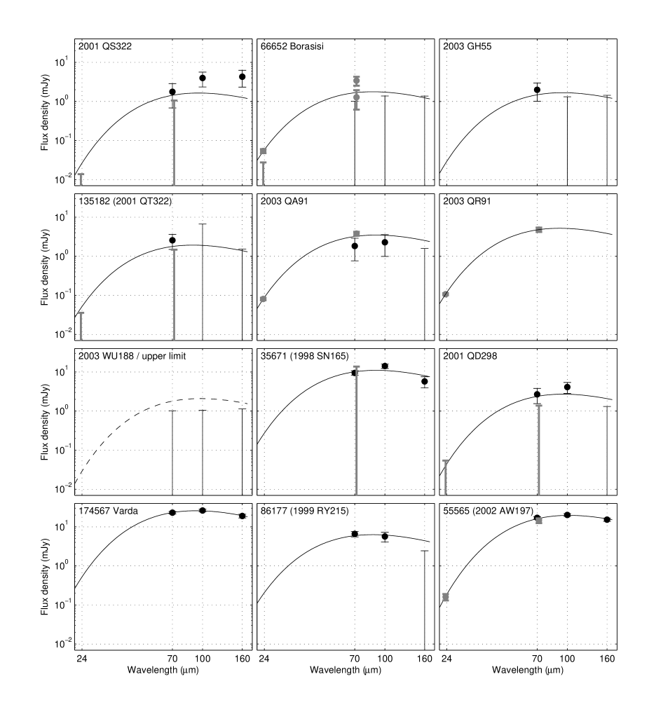
Figure 1: SEDs calculated from the model solutions (Table 5). The black data points are from PACS (70, 100 and $160\ \mathrm{\mu m}$) and the gray points are from MIPS (23.68 and $71.42\ \mathrm{\mu m}$) normalized to the observing geometry of PACS. Error bars without a data point indicate 1$\sigma$ upper limits. An upper-limit solution based on a non-detection is marked with a dashed line (see text). Target 2003 QR₉₁ was not observed by PACS.

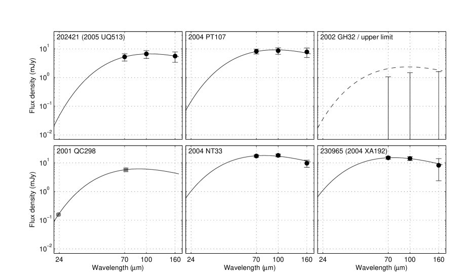
Figure 1: continued. 2002 GH₃₂ has an upper limit solution (see text).

3.3 Comparison with earlier results

Of the 18 targets in our sample only 2001 QD₂₉₈ and 2002 AW₁₉₇ have earlier published diameter/albedo solutions and additionally 2001 QS₃₂₂ and 2001 QT₃₂₂ have upper size limits in the literature. For 2001 QD₂₉₈ the Spitzer/MIPS based result, with different MIPS flux densities and $H_{\mathrm{V}}$ than used in this work (Table 3), was $D$$=$$150_{-40}^{+50}$ km, $p_{\mathrm{V}}$$=$$0.18_{-0.08}^{+0.17}$, $\eta$$=$$0.79_{-0.26}^{+0.28}$ ((Brucker et al., , 2009)). Our new diameter ($233_{-63}^{+27}$ km) is larger and geometric albedo ($0.067_{-0.014}^{+0.062}$) is lower than the previous estimate.

The first size measurement of 2002 AW₁₉₇ was done with the Max Planck Millimeter Bolometer at the IRAM 30 m telescope. The result of Margot et al. (2002) was $D$$=$$886_{-131}^{+115}$ km and $p_{\mathrm{R}}$$=$$0.101_{-0.022}^{+0.038}$. Spitzer measurements gave a smaller size $D$$=$$740\pm$$100$ km and $p_{\mathrm{V}}$$=$$0.12_{-0.03}^{+0.04}$ ((Brucker et al., , 2009)). Our new result is close to this and has significantly smaller error bars ($D$$=$$768_{-38}^{+39}$ km, $p_{\mathrm{V}}$$=$$0.112_{-0.011}^{+0.012}$).

The previous limits of 2001 QS₃₂₂ were $D$$<$200 km and $p_{\mathrm{V}}$$>$$0.15$ ((Brucker et al., , 2009)). While the diameter limit is compatible with the new size estimate ($186_{-24}^{+99}$ km) the new geometric albedo is lower ($0.095_{-0.060}^{+0.531}$) due to PACS data points and updated $H_{\mathrm{V}}$. Also the MIPS data has been reanalysed and has changed for this target. Similarly, the geometric albedo estimate of 2001 QT₃₂₂ is now $0.085_{-0.052}^{+0.424}$ which is lower than the previous lower limit of 0.21 ((Brucker et al., , 2009)). We use a different absolute visual magnitude $H_{\mathrm{V}}$$=$$7.29\pm 0.67$, whereas Brucker et al. (2009) used $6.4\pm 0.5$ for 2001 QT₃₂₂.

For binary targets it is possible to estimate a size range based on the assumptions of spherical shapes and equal albedos of the primary and secondary components. Assuming a bulk density range of 0.5-2.0 g cm^-3 and using the system mass and brightness difference from Grundy et al. (2011) the diameter range for Borasisi (primary component) is 129–205 km. Our solution for the Borasisi-Pabu system is $163_{-66}^{+32}$ km and the derived density $2.1_{-1.2}^{+2.6}$ g cm^-3 (see Section 4.6). Our new estimate for the primary component is $126_{-51}^{+25}$ km (Table 9).

We have remodeled Teharonhiawako (from (Vilenius et al., , 2012)) with updated Spitzer/MIPS flux densities given in Table 3. The updated result gives a 24% larger size and 34% smaller albedo (See Fig. 2 and Tables 6–7 for all results). Previously, MIPS data reduction gave upper limits only for 2001 QY₂₉₇. After updated data reduction from both instruments the solution of 2001 QY₂₉₇ is now based on a floating-$\eta$ fit instead of a fixed-$\eta$ as was the case previously in Vilenius et al. (2012). The new albedo estimate is lower, and the new size estimate is 15% larger. Altjira, which has updated PACS flux densities, is now estimated to be 29% larger than in (Vilenius et al., , 2012). The dynamically hot CKBOs 1996 TS₆₆ and 2002 GJ₃₂, which have only Spitzer observations ((Brucker et al., , 2009)), have been remodeled (see Table 7) after significant changes in flux densities. In our new estimates target 2002 GJ₃₂ has low albedo and large size, whereas the result of Brucker et al. (2009) was a smaller target with moderately high albedo. Contrary, 1996 TS₆₆’s new size estimate is smaller than the previous one, with higher albedo.

Due to the different treatment of upper limits (Section 3.1.1) the size estimates of 2000 OK₆₇, 2001 XR₂₅₄, 2002 KW₁₄, and 2003 UR₂₉₂ have changed while input values in the modeling are the same as in Vilenius et al. (2012) (see Tables 6-7 and Fig. 2). The authors of that work had ignored all three upper limits of 2002 KW₁₄ to obtain a floating-$\eta$ fit for this target but with the new treatment of upper limits there is no need to ignore any data. Instead of a 319 km target with geometric albedo 0.08 the new solution gives a high geometric albedo of 0.31 and a diameter of 161 km. The only case where we have ignored one upper limit is 2000 OK₆₇, which has four upper limits and was not detected by PACS. The upper limit at 160 $\mu m$ is an outlier compared to the others at 70-100 $\mu m$ and therefore we do not assume that band to be close to the detection limit (see the adopted solution in Fig. 2).

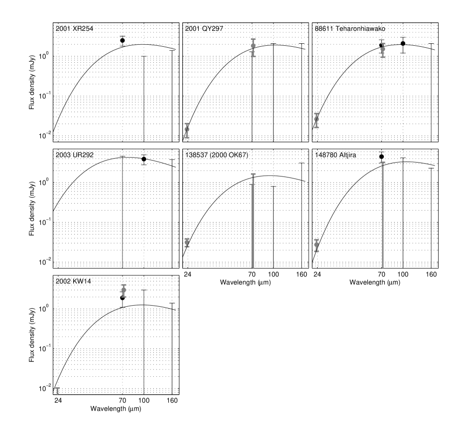
Figure 2: SEDs calculated for remodeled targets from Vilenius et al. (2012). Spitzer data (gray points at 24 and 71 $\mu m$) have been reduced to Herschel observing geometry.

4 Sample results and discussion

In planning the Herschel observations we used a default assumption for geometric albedo of 0.08. As seen in Tables 6-7, almost all dynamically cold CKBOs and more than half of hot CKBOs have higher albedos implying lower flux densities at far-infrared wavelengths. This has lead to the moderate SNRs and several upper limit flux densities in our sample. The frequency of binaries among the cold CKBOs is high due to the selection process of Herschel targets (see Section 2.1). We use this sample of cold CKBOs, affected by the binarity bias, in the debiasing procedure of their size distribution because of the very small number of non-binaries available. In the analysis of sample properties of CKBOs we sometimes use a restricted sample, which we call “regular” CKBOs, where dwarf planets (Quaoar, Varuna, Makemake) and Haumea family members (Haumea and 2002 TX₃₀₀) have been excluded. All five targets mentioned are dynamically hot so that no cold CKBOs are excluded when analysing the “regular CKBOs“ sample.

Table 6: Adopted physical properties of cold classical TNOs.

Target		i ($\degr$)	a (AU)	D (km)	pV	$\eta$	No. of bands	Reference
(2001 QS322)		0.2	44.2	$186_{-24}^{+99}$	$0.095_{-0.060}^{+0.531}$	(fixed)	5	This work
66652 Borasisi (1999 RZ253)	B	0.6	43.9	$163_{-66}^{+32}$	$0.236_{-0.077}^{+0.438}$	$0.77_{-0.47}^{+0.19}$	5	This work
(2003 GH55)		1.1	44.0	$178_{-56}^{+21}$	$0.150_{-0.031}^{+0.182}$	(fixed)	3	This work
(2001 XR254)	B	1.2	43.0	$221_{-71}^{+41}$	$0.136_{-0.044}^{+0.168}$	(fixed)	3	(*) Vilenius et al. (2012)
275809 (2001 QY297)	B	1.5	44.0	$229_{-108}^{+22}$	$0.152_{-0.035}^{+0.439}$	$1.52_{-0.92}^{+0.22}$	5	(*) Vilenius et al. (2012)
(2002 VT${}_{130})$	B	1.2	42.7	$324_{-68}^{+57}$	$0.097_{-0.049}^{+0.098}$	1.20$\pm$0.35	2	Mommert (2013)
(2001 QB${}_{298})$		1.8	42.6	$196_{-53}^{+71}$	$0.167_{-0.082}^{+0.162}$	1.20$\pm$0.35	2	Mommert (2013)
(2001 RZ143)	B	2.1	44.4	$140_{-33}^{+39}$	$0.191_{-0.045}^{+0.066}$	$0.75_{-0.19}^{+0.23}$	5	Vilenius et al. (2012)
(2002 GV31)		2.2	43.9	$<$180	$>$0.19	(fixed)	3	(*) Vilenius et al. (2012)
79360 Sila	B	2.2	43.9	$343\pm 42$	$0.090_{-0.017}^{+0.027}$	$1.36_{-0.19}^{+0.21}$	5	Vilenius et al. (2012)
(2003 QA91)	B	2.4	44.5	$260_{-36}^{+30}$	$0.130_{-0.075}^{+0.119}$	$0.83_{-0.15}^{+0.10}$	5	This work
88611 Teharonhiawako	B	2.6	44.2	$220_{-44}^{+41}$	$0.145_{-0.045}^{+0.086}$	$1.08_{-0.28}^{+0.30}$	5	(*) Vilenius et al. (2012)
(2005 EF298)	B	2.9	43.9	$174_{-32}^{+27}$	$0.16_{-0.07}^{+0.13}$	(fixed)	3	Vilenius et al. (2012)
(2003 QR91)	B	3.5	46.6	$280_{-30}^{+27}$	$0.054_{-0.028}^{+0.035}$	$1.20_{-0.12}^{+0.10}$	2	This work
(2003 WU188)	B	3.8	44.3	$<$220	$>$0.15	(fixed)	3	This work

Table 7: Adopted physical properties of hot classical TNOs.

Target		i ($\degr$)	a (AU)	D (km)	pV	$\eta$	No. of bands	Reference
2002 KX14		0.4	38.9	$455\pm 27$	$0.097_{-0.013}^{+0.014}$	$1.79_{-0.15}^{+0.16}$	5	Vilenius et al. (2012)
2001 QT322		1.8	37.2	$159_{-47}^{+30}$	$0.085_{-0.052}^{+0.424}$	(fixed)	5	This work
2003 UR292		2.7	32.6	$136_{-26}^{+16}$	$0.105_{-0.033}^{+0.081}$	(fixed)	3	(*) Vilenius et al. (2012)
1998 SN165		4.6	38.1	$393_{-38}^{+39}$	$0.060_{-0.013}^{+0.019}$	(fixed)	4	This work
2000 OK67		4.9	46.8	$164_{-45}^{+33}$	$0.169_{-0.052}^{+0.159}$	(fixed)	5	(*) Vilenius et al. (2012)
2001 QD298		5.0	42.7	$233_{-63}^{+27}$	$0.067_{-0.014}^{+0.062}$	(fixed)	5	This work
148780 Altjira	B	5.2	44.5	$331_{-187}^{+51}$	$0.0430_{-0.0095}^{+0.1825}$	$1.62_{-0.83}^{+0.24}$	5	(*) Vilenius et al. (2012)
1996 TS66		7.3	44.2	$159_{-46}^{+44}$	$0.179_{-0.070}^{+0.173}$	$0.75_{-0.27}^{+0.21}$	2	(*) Brucker et al. (2009)
50000 Quaoar	B	8.0	43.3	$1074\pm 38$	$0.127_{-0.009}^{+0.010}$	$1.73\pm 0.08$	8	Fornasier et al. (2013)
2002 KW14		9.8	46.5	$161_{-40}^{+35}$	$0.31_{-0.094}^{+0.281}$	(fixed)	5	(*) Vilenius et al. (2012)
2002 GJ32		11.6	44.1	$416_{-78}^{+81}$	$0.035_{-0.011}^{+0.019}$	$2.05_{-0.36}^{+0.38}$	2	(*) Brucker et al. (2009)
2001 KA77		11.9	47.3	$310_{-60}^{+170}$	$0.099_{-0.056}^{+0.052}$	$2.52_{-0.83}^{+0.18}$	5	Vilenius et al. (2012)
19521 Chaos		12.0	46.0	$600_{-130}^{+140}$	$0.050_{-0.016}^{+0.030}$	$2.2_{-1.1}^{+1.2}$	4	Vilenius et al. (2012)
2002 XW93		14.3	37.6	$565_{-73}^{+71}$	$0.038_{-0.025}^{+0.043}$	$0.79_{-0.24}^{+0.27}$	3	Vilenius et al. (2012)
20000 Varuna		17.2	43.0	$668_{-86}^{+154}$	$0.127_{-0.042}^{+0.040}$	$2.18_{-0.49}^{+1.04}$	3	Lellouch et al. (2013)
2002 MS4		17.7	41.7	$934\pm 47$	$0.051_{-0.022}^{+0.036}$	$1.06\pm 0.06$	5	Vilenius et al. (2012)
2005 RN43		19.2	41.8	$679_{-73}^{+55}$	$0.107_{-0.018}^{+0.029}$	(fixed)	3	Vilenius et al. (2012)
2002 UX25	B	19.4	42.8	$697\pm 35$	$0.107\pm 0.010$	$1.07_{-0.05}^{+0.08}$	8	Fornasier et al. (2013)
174567 Varda	B	21.5	45.6	$792_{-84}^{+91}$	$0.102_{-0.020}^{+0.024}$	$0.84_{-0.22}^{+0.28}$	3	This work
2004 GV9		22.0	41.8	$680\pm 34$	$0.0770_{-0.0077}^{+0.0084}$	$1.93_{-0.07}^{+0.09}$	5	Vilenius et al. (2012)
1999 RY215		22.2	45.5	$263_{-37}^{+29}$	$0.0388_{-0.0065}^{+0.0122}$	(fixed)	3	This work
120347 Salacia	B	23.9	42.2	$901\pm 45$	$0.044_{-0.004}^{+0.004}$	$1.16\pm 0.03$	8	Fornasier et al. (2013)
2002 AW197		24.4	47.2	$768_{-38}^{+39}$	$0.112_{-0.011}^{+0.012}$	$1.29_{-0.10}^{+0.13}$	5	This work
2005 UQ513		25.7	43.5	$498_{-75}^{+63}$	$0.202_{-0.049}^{+0.084}$	(fixed)	3	This work
2002 TX300		25.8	43.5	$286\pm 10$	$0.88_{-0.06}^{+0.15}$	$1.15_{-0.74}^{+0.55}$	occultation	Elliot et al. (2010),
							+3	Lellouch et al. (2013)
2004 PT107		26.1	40.6	$400_{-51}^{+45}$	$0.0325_{-0.0066}^{+0.0111}$	(fixed)	3	This work
2002 GH32		26.7	41.9	$<$ 180	$>$ 0.13	(fixed)	3	This work
136108 Haumea	B	28.2	43.1	$1240_{-59}^{+69}$	$0.804_{-0.095}^{+0.062}$	$0.95_{-0.26}^{+0.33}$	3	(Fornasier et al., , 2013)
136472 Makemake		29.0	45.5	$1430\pm 9$	0.77$\pm$0.03	$2.29_{-0.40}^{+0.46}$	occultation	Ortiz et al. (2012),
							+3	Lellouch et al. (2013)
2001 QC298	B	30.6	46.3	$303_{-30}^{+27}$	$0.061_{-0.017}^{+0.027}$	$0.985_{-0.095}^{+0.084}$	2	This work
2004 NT33		31.2	43.5	$423_{-80}^{+87}$	$0.125_{-0.039}^{+0.069}$	$0.69_{-0.32}^{+0.46}$	3	This work
2004 XA192		38.1	47.4	$339_{-95}^{+120}$	$0.26_{-0.15}^{+0.34}$	$0.62_{-0.49}^{+0.79}$	3	This work

4.1 Measured sizes

The diameter estimates in the ”regular CKBO” sample are ranging from 136 km of 2003 UR₂₉₂ up to 934 km of 2002 MS₄. The not detected targets (2002 GV₃₁, 2003 WU₁₈₈ and 2002 GH₃₂) may be smaller than 2003 UR₂₉₂. Dynamically cold targets in our measured sample are limited to diameters of 100-400 km whereas hot CKBOs have a much wider size distribution up to sizes of $\sim$900 km in our measured ”regular CKBO” sample and up to 1430 km when dwarf planets are included.

We show the cumulative size distribution $N(>$$D)\propto D^{1-q}$ of hot classicals (from Table 7) and cold classicals (from Table 6) in Fig. 3 . In the measured, biased, size distribution of hot CKBOs we can distinguish three regimes for the power law slope: $100$$<$$D$$<$$300\ \mathrm{km}$, $400$$<$$D$$<$$600\ \mathrm{km}$ and $700$$<$$D$$<$$1300\ \mathrm{km}$. The slope parameters for the latter two regimes are $q$$\approx$2.0 and $q$$\approx$4.0. In the small-size regime there are not enough targets in different size bins to derive a reliable slope. The measured, biased, cold CKBO sample gives a slope of $q$$\approx$4.3 in the size range 200$<$$D$$<$300 km. The debiased size distribution slopes are given in Section 4.3.

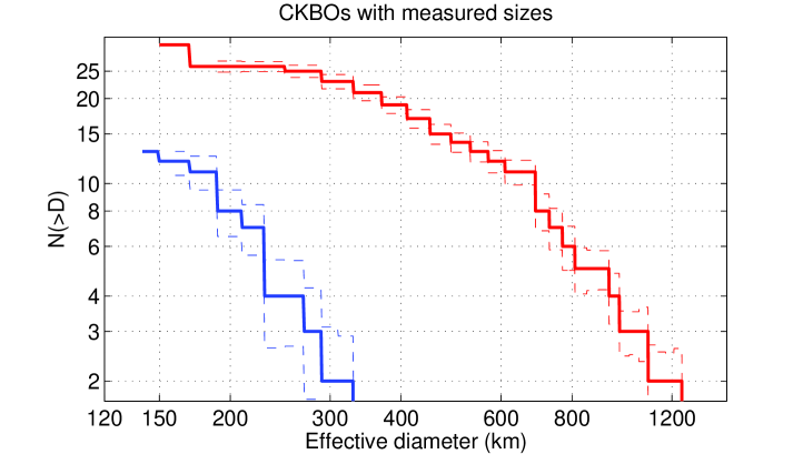
Figure 3: Cumulative size distribution of all measured dynamically hot (red, upper) classicals from Table 7 and dynamically cold (blue, lower) classicals from Table 6. The dotted lines are uncertainties obtained by a Monte Carlo technique where the sizes of targets are varied using their measured error bars, and a set of size distributions are created. The standard deviation of these size distributions is calculated at each size bin.

4.2 Measured geometric albedos

Haumea family members and many dwarf planets have very high geometric albedos. The highest-albedo regular CKBO is 2002 KW₁₄ with $p_{\mathrm{V}}$$=$0.31 and the darkest object is 2004 PT₁₀₇ with $p_{\mathrm{V}}$$=$0.0325, both dynamically hot. Among dynamically cold objects geometric albedo is between Sila’s $p_{\mathrm{V}}$$=$0.090 and Borasisi’s $p_{\mathrm{V}}$$=$0.236.

The sub-sample of cold CKBOs are lacking low-albedo objects compared to the hot sub-sample. Fig. 4 shows probability density functions constructed from the measured geometric albedos and their asymmetric error bars using the technique described in detail in Mommert (2013). The probability density for each individual target is assumed to follow a lognormal distribution, whose scale parameter is calculated using the upper and lower uncertainties given for the measured geometric albedo. The median geometric albedo of the combined probability density (Fig. 4) of cold classicals is $0.14_{-0.07}^{+0.09}$, of regular hot CKBOs $p_{\mathrm{V}}$$=$$0.085_{-0.045}^{+0.084}$, and of all hot CKBOs including dwarf planets and Haumea family the median is $p_{\mathrm{V}}$$=$$0.10^{+0.16}_{-0.06}$. These medians are compatible with averages obtained from smaller sample sizes: $0.17$$\pm$0.04 for cold CKBOs and $0.11$$\pm$0.04 for hot CKBOs in Vilenius et al. (2012) but the difference between the dynamically cold and hot sub-samples is smaller than previously reported.

Of the other dynamical classes, the Plutinos have an average albedo of 0.08$\pm$0.03 ((Mommert et al., , 2012)), scattered disk objects have 0.112 ((Santos-Sanz et al., , 2012)), detached objects have 0.17 ((Santos-Sanz et al., , 2012)), gray Centaurs have 0.056 (Duffard et al. (2013)) and red Centaurs 0.085 (Duffard et al. (2013)). Dynamically hot classicals have a similar average albedo as Plutinos and red Centaurs whereas the average albedo of cold CKBOs is closer to the detached objects.

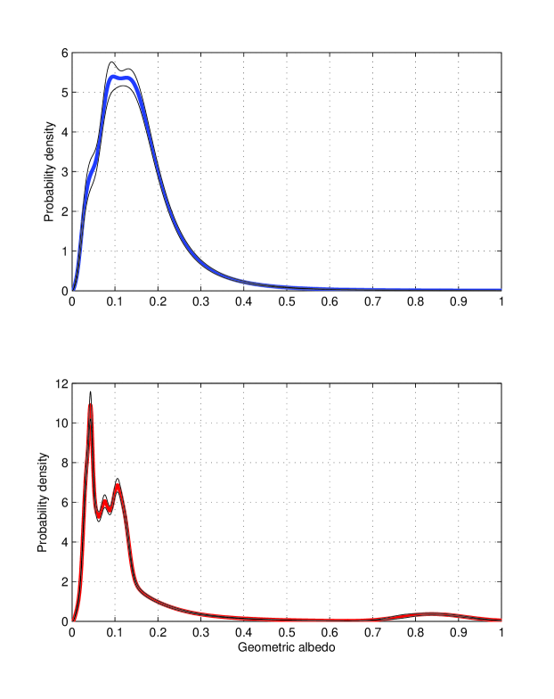
Figure 4: Distribution of measured geometric albedos: upper panel for cold CKBOs and lower panel for hot CKBOs. The thin lines show the standard deviation of all probability density distributions, where each of the distributions has been determined with one target excluded, each target having been excluded once.

4.3 Debiased size distributions

The measured size distributions are affected by biases: the radiometric method has a detection limit, and the measured sample is not representative of all those targets which could have been detectable in principle. For the debiasing we use a synthetic model of outer Solar System objects by the Canada-French Ecliptic Plane Survey (CFEPS, Petit et al., (2011)), which is based on well-calibrated optical surveys. CFEPS provides $H_{g}$ magnitudes and orbital parameters of more than 15000 cold CKBOs and 35000 hot synthetic CKBOs. We perform a two-stage debiasing of the measured size distribution (see Appendix A for details) and derive slope parameters. We have constructed a model of the detection limit of Herschel observations, which depends on objects’ sizes, albedos and distances. This model is used in the first stage of debiasing. In the second stage we debias the size distribution in terms of how the distribution of $H_{g}$s of the measured targets are related to the $H_{g}$ distribution of the synthetic sample of those objects, which would have been detectable.

CFEPS has synthetic objects to the limit of $H_{g}$=8.5. All cold CKBOs in our measured sample have $H_{g}<$7.5 and all hot CKBOs have $H_{g}<$8.0. Therefore, these limits are first applied to the CFEPS sample before debiasing the size distributions. Since all of the measured hot CKBOs are in the inner or main classical belts, we exclude the outer CKBOs of CFEPS in the debiasing. Furthermore, we have excluded a few measured targets which are outside the orbital elements space of CFEPS objects, or which are close to the limit of dynamically cold/hot CKBOs, to avoid contamination from one sub-population to the other.

In translating the optical absolute magnitude of simulated CFEPS objects into sizes, a step needed in the debiasing (Appendix A), we use the measured albedo probability densities (Fig.  4) in a statistical way. Our measured dynamically hot CKBOs cover the relevant heliocentric distance range of inner and main classical belt CFEPS objects. While our measured sample of cold CKBOs is limited to 38$<$$r$$<$45 AU we assume that the shape of the albedo distribution applies also to more distant cold CKBOs. Although there is an optical discovery bias prefering high-$p_{V}$ objects at large distances, the radiometric method has an opposite bias: low-$p_{V}$ objects are easier to detect at thermal wavelengths than high-$p_{V}$ objects. Among the radiometrically measured targets we do not find evidence of any significant correlations (see Section 4.5) between geometric albedo and orbital elements, heliocentric distance at discovery time nor ecliptic latitude at discovery time.

The debiased size distributions are shown in Fig. 5. Our analysis of cold CKBOs gives a debiased slope of $q$=5.1$\pm$1.1 in the range of effective diameters of 160$<$$D$$<$280 km. In the measured sample there are seven binaries and three non-binaries in this size range. For dynamically hot CKBOs the slope is $q$=2.3$\pm$0.1 in the size range 100$<$$D$$<$500 km. The slope is steepening towards the end tail of the size distribution and in the size range 500$<$$D$$<$800 km we obtain a slope parameter of $q$=4.3$\pm$0.9. When comparing the slopes of the cold and hot sub-populations it should be noted that for the cold subsample we are limited to the largest objects and the maximum size of cold CKBOs is smaller than that of hot CKBOs.

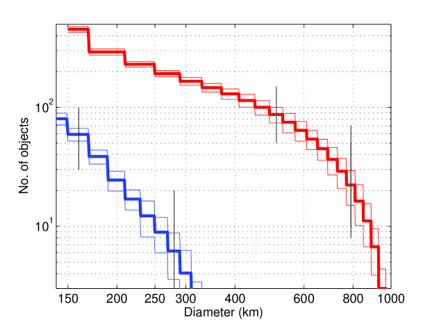
Figure 5: Debiased size distributions (see text): hot CKBOs (red, upper) and cold CKBOs (blue, lower). The thin red and blue lines are the error bars of each size bin (bin size 20 km for dynamically cold and 40 km for dynamically hot CKBOs). The vertical lines mark the ranges for which slope parameters have been determined.

Size distribution is often derived from the LF using simplifying assumptions about common albedo and distance. Fraser et al. (2010) have derived a LF based slope for dynamically cold objects ($i$$<$5 deg, 38$<$$r$$<$55 AU): $q$=5.1$\pm$1.1, which is well compatible with our value from a debiased measured size distribution. For dynamically hot CKBOs Fraser et al. (2010) derived two slopes depending on the distance of objects. For dynamically hot objects with 38$<$$r$$<$55 AU and $i$$>$5 deg: $q$$=$2.8$\pm 1.0$ and for a combined sample of these hot and “close” objects (30$<$$r$$<$38 AU): $q$$=$3.0$\pm 0.6$. Both of the LF based results are compatible within the given uncertainties with our estimate of $q$=2.3$\pm$0.1.

4.4 Beaming factors

The temperature distribution over an airless object affects the observed SED shape. In the NEATM model temperature is adjusted by the beaming factor $\eta$ as explained in Section 3.1. For CKBOs, the PACS bands are close to the thermal peak of the SED whereas MIPS provides also data from the short-wavelength part of the SED. Therefore, in order to determine a reliable estimate for the average beaming factor of classical TNOs we select those solutions which are based on detections with both PACS and MIPS and detected in at least three bands. Furthermore, we require that the MIPS 24 $\mu m$ band has been detected because it constrains the overall shape of the SED making inferences based on those results more reliable. There is a large scatter of beaming factors among CKBOs spanning the full range of $0.6$$<$$\eta$$<$$2.6$. There are five cold CKBOs and eight hot CKBOs with floating-$\eta$ solutions fulfilling the above mentioned criteria. The averages of the two subpopulations do not differ much compared to the standard deviations. The average beaming factor of 13 cold and hot CKBOs is $\eta$$=$1.45$\pm$0.46 and the median is 1.29. This average is very close to the previous average based on eight targets: $\eta$$=$1.47$\pm$0.43 ((Vilenius et al., , 2012)). The new average $\eta$ is compatible with the default value of 1.20$\pm$0.35 for fixed $\eta$ fits as well as with averages of other dynamical classes: seven Plutinos have the average $\eta$$=$$1.11_{-0.19}^{+0.18}$ ((Mommert et al., , 2012)) and seven scattered and detached objects have $\eta$$=$1.14$\pm$0.15 ((Santos-Sanz et al., , 2012)). Statistically, beaming factors of a large sample of TNOs from all dynamical classes are dependent on heliocentric distance ((Lellouch et al., , 2013)). Therefore, $\eta$ values are likely to differ due to different distances of the populations in different dynamical classes.

4.5 Correlations

In the sample of measured objects we have checked possible correlations between geometric albedo $p_{\mathrm{V}}$, diameter $D$, orbital elements (inclination $i$, eccentricity $e$, semimajor axis $a$, perihelion distance $q$), beaming factor $\eta$, heliocentric distance at discovery time, ecliptic latitude at discovery time, visible spectral slope, as well as B-V, V-R and V-I colors. We use a modified form of the Spearman correlation test (Spearman (1904)) taking into account asymmetric error bars and small numbers statistics. The details of this method are described in Peixinho et al. (2004) and Santos-Sanz et al. (2012, Appendix B.2.). We consider correlation coefficient $\rho$ to show a ’strong correlation’ when $|\rho|\geq 0.6$ and ’moderate correlation’ when $0.3\leq|\rho|<0.6$. Our correlation method does not show any significant (confidence on the presence of a correlation $>$3$\sigma$) correlations between any parameters within the dynamically cold subpopulation with $N$=13 targets. Similarly, when making the correlation analysis on the CKBOs according to the DES classification (N=23) we do not find any significant correlations.

4.5.1 Diameter and geometric albedo

There is a lack of large objects at small inclinations and of small objects at high inclinations in our measured sample. The latter are subject to discovery biases since many of the surveys have been limited close to the ecliptic plane ($H_{V}$ and ecliptic latitude at discovery time show a moderate anti-correlation in the sample of all radiometrically measured targets). There is a strong size-inclination correlation when all targets are included (4.4$\sigma$), and a moderate correlation if dwarf planets and Haumea family are excluded (3.9$\sigma$). The strong correlation within the sub-sample of hot CKBOs reported by Vilenius et al. (2012) is only moderate with our larger number of targets, and it is no longer significant (2.3-2.5$\sigma$). Levison and Stern (2001) found the presumable size-inclination trend from the correlation between intrinsic brightness and inclination and showed that their result is unlikely to be caused by biases. When observing with the radiometric techniques, there is a selection bias of targets, which we estimate to have high enough flux density to be detectable. According to Equation (3) the observed flux is approximately proportional to the projected area and inversely proportional to the square of distance. A statistical study of 85 TNOs and Centaurs, with partially overlapping samples with this work, showed a strong ($\rho$$=$0.78, significance $>$8$\sigma$) correlation between diameter and instantaneous heliocentric distance ((Lellouch et al., , 2013)). Dynamically hot CKBOs show a moderate correlation between effective diameter and heliocentric distance at discovery time (3.2$\sigma$). However, it is not significant when analyzed without dwarf planets and Haumea family (the ”regular“ sub-sample). A diameter/inclination correlation could appear if there is a correlation between diameter and distance as well as between distance and inclination. Our analysis finds no evidence of a correlation between inclination and heliocentric distance for the whole measured sample ($\rho$$=$0.20, significance 1.2$\sigma$) or any of the sub-samples. Therefore, we consider the correlation between diameter and inclination reported here not to be caused by a selection bias.

There is a moderate ($\rho$$\approx$-0.5) anti-correlation between diameter and geometric albedo among the “regular” CKBOs (3.4$\sigma$). This correlation disappears when the dwarf planets and Haumea family members are added, or when the “regular” CKBOs is divided into its cold or hot components. Inclination may be a common variable, which correlates both with diameter and tentatively with albedo as explained in the following. There is a moderate anticorrelation between inclination and albedo among the “regular” CKBOs, although it is not considered significant (2.5$\sigma$). This is probably caused mainly by the cold CKBOs ($\rho$=-0.51, 1.8$\sigma$, N=13) and less by the “regular” hot CKBOs ($\rho$=-0.17, 0.8$\sigma$, N=26). When combining the significant diameter/inclination correlation (3.9$\sigma$) with a tentative albedo/inclination correlation this combination may explain the moderate diameter/albedo anti-correlation we observe in our “regular” CKBOs sample. Therefore, we do not confirm the finding of Vilenius et al. (2012) about an anti-correlation between size and albedo within the classical TNOs as it is probably due to a bias. The anti-correlation between size and albedo was not observed in Plutinos ((Mommert et al., , 2012)), which do not show any correlation between size and albedo, nor with scattered/detached-disc objects which show a positive correlation instead ((Santos-Sanz et al., , 2012)).

We find no evidence of other correlations with orbital elements or colors involving size or geometric albedo.

4.5.2 Other correlations

CKBOs are known to have an anti-correlation between surface color/spectral slope and orbital inclination (Trujillo and Brown, (2002), (Hainaut and Delsanti, , 2002)). In our measured sample a moderate correlation exists for the whole sample (3.2$\sigma$) but is not significant for the “regular” CKBOs (2.0$\sigma$), which do not include dwarf planets and Haumea family members. We do not find any correlations of the B-V, V-R and V-I colors with parameters other than spectral slope.

The apparent $H_{\mathrm{V}}$ vs $i$ anti-correlation in our target sample mentioned in Section 2.1 is moderate and significant for the whole sample (3.9$\sigma$) as well as for the hot sub-population (3.1$\sigma$), but less significant on the “regular” hot CKBOs sub-sample (2.5$\sigma$).

4.6 Binaries

In deriving bulk densities of binary systems, whose effective diameter $D$ has been determined by the radiometric method, we assume that the primary and secondary components i) are spherical, and ii) have equal albedos. A known brightness difference between the two components $\Delta V$ can be written as $k=10^{-0.2\Delta\mathrm{V}}=\frac{D_{2}}{D_{1}}/l$, where $D_{1}$ and $D_{2}$ are the diameters of the primary and the secondary component and $l=\sqrt{p_{\mathrm{V1}}/p_{\mathrm{V2}}}$ (components’ geometric albedos $p_{\mathrm{V1}}$ and $p_{\mathrm{V2}}$). The radiometric (area-equivalent) effective diameter of the system is $D^{2}=D_{1}^{2}+D_{2}^{2}$ and the “volumetric diameter” is $D_{\mathrm{Vol}}=\frac{\left(1+\left(kl\right)^{3}\right)^{1/3}}{\sqrt{1+\left(kl\right)^{2}}}D$, which is then used in calculating mass densities: $\frac{6m}{\pi D_{\mathrm{Vol}}^{3}}$ with the usual assumption that l equals unity. The new radiometric mass density estimates of Borasisi, Varda and 2001 QC₂₉₈, and updated (see Section 3.3) densities of Teharonhiawako, Altjira, 2001 XR₂₅₄, and 2001 QY₂₉₇ are given in Table 8 and shown in Fig. 6. When $\Delta V$ is small, the density estimate does not change to significantly higher densities by changing the assumed ratio of geometric albedos unless the albedo contrast between the primary and the secondary was extreme. The sizes of the binary components (Table 9) for $<$400 km objects are not significantly different from each other. If we make the assumption that $D_{1}=D_{2}$ and determine densities and relative albedos we get densities close to those in Table 8 for the $<$400 km objects and albedo ratios of 1.1-1.9.

The new density estimates of four targets are lower than those determined by Vilenius et al. (2012). The reason for the large change in density estimates is the Spitzer flux update of three of the targets and a different technique of treating upper limits in the cases of Teharonhiawako, Altjira and 2001 XR₂₅₄. Our assumption that the objects are spherical may give too low density estimates for elongated objects. The relatively large light curve variation of 2001 QY₂₉₇ of $\sim$0.5 mag (Thirouin et al. 2012) suggests a shape effect whereas the light curve amplitude of Altjira is not well known and is probably $<$0.3 mag (Sheppard (2007)). Lower density limits can be derived based on rotational properties but the period is not known for these two targets. Densities lower than that of water ice have been reported for TNOs in the literature (e.g. Stansberry et al. (2006)). The density of a sphere of pure water ice under self-compression is slightly less than 1 g cm^-3 and porosity at micro and macro scales reduces the bulk density. Another common low-density ice is methane with a density of $\sim$0.5 g cm^-3. A statistical study of TNOs from all dynamical classes shows that their surfaces are very porous ((Lellouch et al., , 2013)) indicating that the material on the surface has a low density. However, the low bulk densities of Altjira and Teharonhiawako reported here require significant porosities of 40-70% for material densities of 0.5-1.0 g cm^-3. This would indicate the presence of macroporosity, i.e. that the objects are rubble piles of icy pieces.

Table 8: Density estimates of classical TNO binaries with a known mass. The primary and secondary are assumed to have equal albedos and equal densities.

Target	Adopted $\Delta$V	Mass	Bulk density / literature	Reference	Bulk density / this work
	(mag)	($\times 10^{18}$ kg)	(g cm-3)		(g cm-3)
Borasisi	0.45	$3.433\pm 0.027$	…	…	$2.1_{-1.2}^{+2.6}$
2001 XR254	0.43	$4.055\pm 0.065$	$1.4_{-1.0}^{+1.3}$	Vilenius et al. (2012)	$1.00_{-0.56}^{+0.96}$
2001 QY297	0.20	$4.105\pm 0.038$	$1.4_{-1.3}^{+1.2}$	Vilenius et al. (2012)	$0.92_{-0.27}^{+1.30}$
Sila	0.12	$10.84\pm 0.22$	0.73$\pm$0.28	Vilenius et al. (2012), (b)	…
Teharonhiawako	0.70	$2.445\pm 0.032$	$1.14_{-0.91}^{+0.87}$	Vilenius et al. (2012)	$0.60_{-0.33}^{+0.36}$
Altjira	0.23	$3.986\pm 0.067$	$0.63_{-0.63}^{+0.68}$	Vilenius et al. (2012)	$0.30_{-0.14}^{+0.50}$
2002 UX25	$\sim$2.7	$\sim$125$\pm$3	0.82$\pm$0.11	Brown (2013)
Varda	1.45	265.1$\pm$3.9	…	…	$1.27_{-0.44}^{+0.41}$
2001 QC298	0.44	11.88$\pm$0.14	…	…	$1.14_{-0.30}^{+0.34}$
Quaoar	$5.6\pm 0.2$	$1300-1400$	$2.18_{-0.36}^{+0.43}$	Fornasier et al. (2013)	…
Salacia	$2.372\pm 0.060$	$436\pm 11$	$1.29_{-0.23}^{+0.29}$	Fornasier et al. (2013)	…

Table 9: Sizes of primary and secondary components assuming equal albedos and spherical shapes of both components.

Target	Primary’s size	Secondary’s size
	$D_{1}$ (km)	$D_{2}$ (km)
Borasisi	$126_{-51}^{+25}$	$103_{-42}^{+20}$
2001 XR254	$171_{-55}^{+32}$	$140_{-45}^{+26}$
2001 QY297	$169_{-80}^{+16}$	$154_{-73}^{+15}$
Sila	$249_{-31}^{+30}$	$236_{-29}^{+28}$
Teharonhiawako	$178_{-36}^{+33}$	$129_{-26}^{+24}$
Altjira	$246_{-139}^{+38}$	$221_{-125}^{+34}$
2002 UX25	670$\pm$34	193$\pm$10
Varda	$705_{-75}^{+81}$	$361_{-38}^{+42}$
2001 QC298	$235_{-23}^{+21}$	$192_{-19}^{+17}$
Quaoar	$1070\pm 38$	$81\pm 11$
Salacia	$829\pm 30$	$278\pm 10$

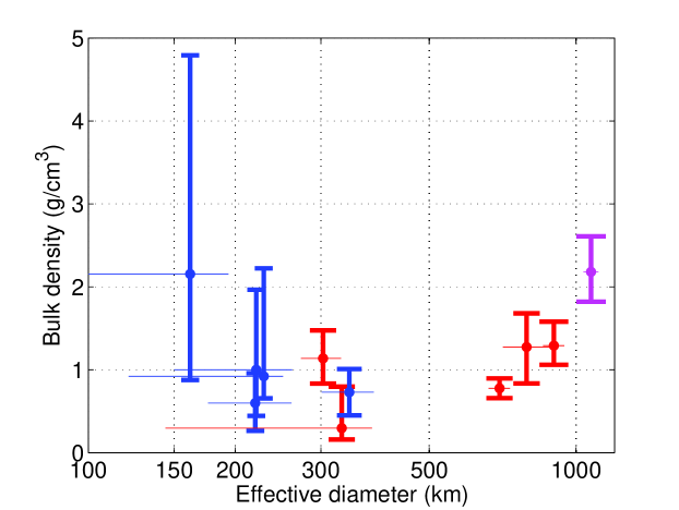
Figure 6: Bulk densities of classical TNOs. Blue marks cold CKBOs, red hot CKBOs, and magenta dwarf planet Quaoar.

5 Conclusions

The Herschel mission and the cold phase of Spitzer have ended. The next space mission capable of far-infrared observations of CKBOs will be in the next decade. Occultations can provide very few new size estimates annually, and the capabilities of the Atacama Large Millimeter Array (ALMA) to significantly extend the sample of measured sizes of TNOs already presented may be limited by its sensitivity.

In this work we have analysed 18 classical TNOs to determine their sizes and albedos using the radiometric technique and data from Herschel and/or Spitzer. We have also re-analysed previously published targets, part of them with updated flux densities. The number of CKBOs with size/albedo solutions in literature and this work is increased to 44 targets and additionally three targets have a diameter upper limit and albedo lower limit. We have determined the mass density of three CKBOs and updated four previous density estimates. Our main conclusions are:

1. The dynamically cold CKBOs have higher geometric albedo ($0.14$) than the dynamically hot CKBOs ($0.085$ without dwarf planets and Haumea family, 0.10 including them), although the difference is not as great as reported by Vilenius et al. (2012).

2. We do not confirm the general finding of Vilenius et al. (2012) that there is an anti-correlation between diameter and albedo among all measured CKBOs as that analysis was based on a smaller number of targets.

3. The cumulative size distributions of cold and hot CKBOs have been infered using a two-stage debiasing procedure. The characteristic size of cold CKBOs is smaller, which is compatible with the hypothesis that the cold sub-population may have formed at a larger heliocentric distance than the hot sub-population. The cumulative size distribution’s slope parameters of hot CKBOs in the diameter range 100$<$$D$$<$500 km is $q$=2.3$\pm$0.1. Dynamically cold CKBOs have an infered slope of $q$$=$5.1$\pm$1.1 in the range 160$<$$D$$<$280.

4. The bulk density of Borasisi is $2.1_{-0.59}^{+0.58}$ g cm^-3, which is higher (but within error bars) than other CKBOs of similar size. The bulk densities of Varda and 2001 QC₂₉₈ are $1.25_{-0.43}^{+0.40}$ g cm^-3 and $1.14_{-0.30}^{+0.34}$ g cm^-3, respectively. Our re-analysis of four targets ($D$$<$400 km) has decreased their density estimates and they are mostly between 0.5 and 1 g cm^-3 implying high macroporosity.

Appendix A Debiasing of size distributions

A.1 Targets

In the debiasing we use those measured targets which are compatible with the orbital element space of CFEPS synthetic objects. Due to different classification used in our observing program, one cold CKBO (2001 QB₂₉₈) and two hot CKBOs from the inner belt (2003 UR₂₉₂ and 2002 XW₉₃) have been excluded from the debiasing. To prevent possible contamination between cold/hot sub-populations we have also excluded four hot CKBOs, whose inclinations are not far above the $i$=4.5 deg cut-off limit (Quaoar, Altjira, 2001 QD₂₉₈ and 2000 OK₆₇). Three measured targets have their semi-major axis within the gap in CFEPS objects reserved for the 2:1 mean motion resonance with Neptune. To our knowledge these three targets are not in resonance, therefore they are included. In total, 25 hot CKBOs from the inner and main belts are included in the debiasing as well as 12 cold CKBOs.

A.2 Magnitude conversion

CFEPS uses $H_{g}$ values for their synthetic objects. If V-R color is known then $H_{g}$ can be converted into $H_{V}$. We use the average color of cold classicals: V-R=0.63$\pm$0.09 (N=49) and hot classicals: V-R=0.51$\pm$0.14 (N=43) from the MBOSS-2 data base. Lupton (2005) conversion formulas and conversion uncertainties are (see Footnote 2 for reference):

$$V=g-0.5784*(g-r)-0.0038,\quad\sigma=0.0054$$ (6)

$$R=r-0.1837*(g-r)-0.0971,\quad\sigma=0.0106.$$ (7)

Using the average V-R color we get

$$\mathrm{cold:}\quad V=g-0.52,\quad\sigma=0.09$$ (8)

$$\mathrm{hot:}\quad V=g-0.40,\quad\sigma=0.14$$ (9)

A.3 PACS detection limit

Many of the measured cold CKBOs were very faint, the flux densities being $<$5.5 mJy. Contrary, the hot CKBOs were brighter and only one out of 29 observed by PACS was a non-detection. The PACS observations were executed in a standardized way using similar observation durations and parameters. While the repetition factor in “TNOs are Cool” was designed separately for each target, in the range REP=1,…,6, for the cold CKBOs the most common choise was REP=5 (total 2-visit duration at 70 $\mu m$ or 100 $\mu m$ band 94 min). Of the cold CKBOs only Sila, Teharonhiawako, 2001 XR254 and 2002 GV31 had shorter durations with REP=3 or REP=4. 2002 GV31 was a non-detection, the other three are large (D$>$200 km) and relatively bright ($H_{V}$$<$6.1). The lowest flux densities with 2-band detections in our sample are at the level of 1.7 mJy at 100 $\mu m$. According to NEATM (in the following we assume $\eta=$1.2), the peak flux density of 1.7 mJy would be emitted by an object at $r_{h}$=$\Delta$=40 AU if its diameter is $D_{\mathrm{ref}}$=167.5 km and geometric albedo $p_{V,\mathrm{ref}}$=0.04. In the following, we make the simplifying assumption that during our observations $r_{h}\approx\Delta$. The peak flux density remains constant (but with a small shift in wavelength position) if a target is at different distance and its size with respect to the reference size is scaled according to the distance change. If $s$ is a scale factor in the distance then the diameter scales as $s^{1.75}$, i.e. at a distance of 40$s$ AU the object’s size should be $s^{1.75}D_{\mathrm{ref}}$ to maintain the same peak flux density. In the above, albedo was kept constant. The effect of albedo depends on the phase integral because we have for the Bond albedo $A$: $A=p_{V}q\left(p_{V}\right)$, where $q\left(p_{V}\right)=0.336p_{V}+0.479$ (Brucker et al. 2009). Other values being constant, if geometric albedo changes then the diameter has to be scaled in order to maintain the constant maximum flux density. If $t$ is the scaling factor of geometric albedo, then diameter scales as

$$\left(\frac{1-p_{V,\mathrm{ref}}\,q(p_{V,\mathrm{ref}})}{1-t\,p_{V,\mathrm{ref}}\,q(t\,p_{V,\mathrm{ref}})}\right)^{\frac{3}{8}}.$$ (10)

A.4 Debiasing procedure

A.4.1 Debiasing stage 1

First we debias with respect to the radiometric detection limit (Section A.3). Diameters are assigned to each CFEPS CKBO in a random way using the geometric albedo probability densities derived from measured targets (see Section 4.2). Then, size distributions of synthetic objects are calculated. The debiasing factors of stage (1) are obtained by dividing the numbers of CFEPS CKBOs in the cumulative size distribution bins by the numbers of potentially detectable CFEPS objects in the same size bins. For each synthetic object we have the distance, randomly selected albedo, and the diameter calculated using that albedo and $H_{g}$. Each object is checked against the detection limit derived in Section A.3. The uncertainties are calculated as the 1$\sigma$ uncertainties of the calculated ratio, where the two distributions have been produced 500 times with randomly assigned albedos to the synthetic objects.

The debiasing factors are applied to the size distributions of measured targets. The numbers of targets in the measured size distribution bins are multiplied by the corresponding stage (1) debiasing factors.

A.4.2 Debiasing stage 2

In stage (2) we are debiasing the selection effects of our target sample compared to the sample which could have been detected with PACS. The selection effects of the measured target sample include the discovery bias of known TNOs. This debiasing is done using optical absolute magnitudes $H_{g}$ of both the synthetic CFEPS objects and the measured targets (steps 1-3 below) and translated into debiasing factors for each bin in the size distribution (steps 4-6). The stage (2) debiasing factors are calculated in the following way:

1. Create cumulative $H_{g}$ distribution of both the measured sample and the potentially detectable CFEPS synthetic objects. The latter is an average of a large number of sets of potentially detectable objects, where the detection limit calculation is using randomly assigned albedos (from the probability density distribution similar to those in Fig. 4) for each synthetic object.

2. Calculate the ratio of numbers of objects in each $H_{g}$ bin of the potentially detectable distribution and the measured distribution. Normalize these factors so that the smallest factor is equal to one.

3. Multiply the measured $H_{g}$ distribution by the factors from step 2.

4. Generate sizes for objects in each $H_{g}$ bin after step 3 in a statistical way using the measured albedo probability density distribution. The relative differences in the numbers of objects in each $H_{g}$ bin of this step is given by the relative differences of numbers of objects in the $H_{g}$ distribution of step 3.

5. Calculate a size distribution using all the objects generated in step 4.

6. Calculate debiasing factors from step 5 and the measured size distribution. Normalize these factors so that the largest target has a factor equal to one. In the dynamically hot sub-population Haumea and Makemake, two targets outside the CFEPS $H_{g}$ range, were not included in calculating debiasing factors.