Model-based construction of Open Non-uniform Cylindrical Algebraic Decompositions

Abstract

In this paper we introduce the notion of an Open Non-uniform Cylindrical Algebraic Decomposition (NuCAD), and present an efficient model-based algorithm for constructing an Open NuCAD from an input formula. A NuCAD is a generalization of Cylindrical Algebraic Decomposition (CAD) as defined by Collins in his seminal work from the early 1970s, and as extended in concepts like Hong’s partial CAD. A NuCAD, like a CAD, is a decomposition of $\mathbb{R}^{n}$ into cylindrical cells. But unlike a CAD, the cells in a NuCAD need not be arranged cylindrically. It is in this sense that NuCADs are not uniformly cylindrical. However, NuCADs — like CADs — carry a tree-like structure that relates different cells. It is a very different tree but, as with the CAD tree structure, it allows some operations to be performed efficiently, for example locating the containing cell for an arbitrary input point.

1 Introduction

This paper introduces a new model-based approach to constructing Cylindrical Algebraic Decompositions (CADs). The model-based approach, building on [4] and [1], has some very nice properties (described later in the paper) that make it appealing. However, prior work has not applied it to constructing CADs. Jovanovic and de Moura’s work [4], which introduced the approach, uses it to determine the satisfiability of Tarski formulas. In some sense, their approach can be seen as building a CAD-like decomposition. However, what is constructed is an unstructured list of cells, which makes it unsuitable for some of what CADs are used for. Moreover, the method is not obviously parallelizable, and it doesn’t take as strong advantage of the “model-based approach” as is possible. [1] shows how to make stronger use of the “model” during the construction of a single open cell. This paper continues in one of the directions outlined in that paper, using the strong model-based approach to construct not just a single cylindrical cell, but a whole decomposition of real space into cylindrical cells.

A particularly exciting aspect of this new model-based approach is that while each cell in the decomposition is cylindrical, those cells need not by cylindrically arranged with respect to one another. This frees us to construct more general decompositions than CADs, thereby representing semi-algebraic sets with fewer cells. To make use of this freedom, we introduce a new generalization of CAD, the Open Non-uniform Cylindrical Algebraic Decomposition (Open NuCAD), and an algorithm TI-Open-NuCAD that efficiently constructs an Open NuCAD from an input formula. As demonstrated by an example computation that is worked out in detail in this paper, the flexibility of NuCADs allow sets to be represented using fewer cells than with a CAD.

2 Non-uniform Cylindrical Algebraic Decomposition

In this section we define Non-uniform Cylindrical Algebraic Decomposition. We assume the reader is already familiar with the usual CAD notions — like delineability, level of a polynomial, etc. Note that $\lambda$ denotes the empty string in what follows, $||$ indicates concatenation, and $\pi_{k}(\cdot)$ denotes projection down onto $\mathbb{R}^{k}$. This paper deals with open cylindrical cells which, except in the trivial case of a single cell, cannot truly decompose $\mathbb{R}^{n}$. Instead, we say that a set of open regions defines a weak decomposition of $\mathbb{R}^{n}$ if the regions are pairwise disjoint, and the union of their closures contains $\mathbb{R}^{n}$. We here provide a definition of an open cylindrical cell. This is entirely in keeping with the usual definition of a cell in the CAD literature.

Definition 1

An Open Cylindrical Cell is a subset of $\mathbb{R}^{n}$ is a set of the form

$$\{(\alpha_{1},\ldots,\alpha_{n})\in B\times\mathbb{R}|f(\alpha_{1},\ldots,\alpha_{n-1})<\alpha_{n}<g(\alpha_{1},\ldots,\alpha_{n-1})\}$$

or

$$\{(\alpha_{1},\ldots,\alpha_{n})\in B\times\mathbb{R}|f(\alpha_{1},\ldots,\alpha_{n-1})<\alpha_{n}\}$$

or

$$\{(\alpha_{1},\ldots,\alpha_{n})\in B\times\mathbb{R}|\alpha_{n}<g(\alpha_{1},\ldots,\alpha_{n-1})\}$$

where $B$ is an open cylindrical cell in $\mathbb{R}^{n-1}$ and the graphs of $f$ and $g$ over $B$ are disjoint sections of polynomials, and $()$ is considered an open cylindrical cell in $\mathbb{R}^{0}$.

Next we define Open Non-uniform Cylindrical Algebraic Decomposition (Open NuCAD), which relaxes the requirements of the usual CAD. In particular, it is possible to have two cells whose projections onto a lower dimension are neither equal nor disjoint. In other words, while each individual cell is cylindrical, distinct cells are not necessarily organized into cylinders.

Definition 2

An Open Non-uniform Cylindrical Algebraic Decomposition (Open NuCAD) of $\mathbb{R}^{n}$ is a collection $C$ of open cylindrical cells, each of which is labelled with a unique string of the form $([0-9]+(L,U,X))*$. The relation

$$E=\{(C_{1},C_{2})|\mbox{$C_{1}$ and $C_{2}$ are cells with labels $lab_{1}$ and $lab_{2}$ satisfying $lab_{2}=lab_{1}([0-9]+(L,U,X))$}\}$$

defines a graph on the cells.

1. the graph $(C,E)$ is a tree, rooted at cell $\mathbb{R}^{n}$, with label $\lambda$ (the empty string),

2. the children of cell $C_{0}$ with label $lab_{0}$ have labels taken from the set

   $$\{lab_{0}1L,\ldots,lab_{0}nL,lab_{0}1U,\ldots,lab_{0}nU,lab_{0}nX\}$$

   and if $C_{0}$ has children, then one of them is labelled $lab_{0}nX$,

3. if cell $C_{2}$ is the child of $C_{1}$ with label $lab_{1}nX$, then $C_{2}\subseteq C_{1}$ and for each $i\in\{1,\ldots,n\}$, in the cylinder over over $\pi_{i-1}(C_{2})$ the section that defines the lower (resp. upper) boundary of $C_{2}$ in $x_{i}$ is either identical to or disjoint from the section that defines the lower (resp. upper) boundary of $C_{1}$ in $x_{i}$

4. if cell $C_{X}$ is the child of $C_{0}$ with label $lab_{0}nX$, then

   $$(\pi_{i-1}(C_{X})\times\mathbb{R})\cap\pi_{i}(C_{0})-\overline{\pi_{i}(C_{X})}$$ (1)

   consists of zero one or two open cells: the region with $i$-coordinates below $\overline{\pi_{i}(C_{X})}$ if it is non-empty, which is denoted $B_{L}$, and the region with $i$-coordinates above $\overline{\pi_{i}(C_{X})}$ if it is non-empty, which is denoted $B_{U}$. There is a cell with label $lab_{0}iL$ if and only if $B_{L}$ is non-empty and, if it exists, that cell is $(B_{L}\times\mathbb{R}^{n-i})\cap C_{0}$. There is a cell with label $lab_{0}iU$ if and only if $B_{U}$ is non-empty and, if it exists, that cell is $(B_{U}\times\mathbb{R}^{n-i})\cap C_{0}$.

Next we prove that NuCADs really do define decompositions of $\mathbb{R}^{n}$ or, more properly, Open NuCADs define weak decompositions of $\mathbb{R}^{n}$.

Theorem 1

If cell $C_{0}$ is a non-leaf node in the graph $(C,E)$, its children form a weak decomposition of $C_{0}$.

Proof. What needs to be proved is that there is no open subset of $C_{0}$ having empty intersection with all of the children of $C_{0}$. Let $S$ be an open, connected subset of $C_{0}$. Let $i$ be the maximum element of $\{1,\ldots,n+1\}$ such that $\pi_{i-1}(S)\subseteq\pi_{i-1}(C_{X})$. If $i=n+1$, then $S$ is contained in $C_{X}$, the child that, by definition, must exist. So the theorem holds in this case.

If $i\leq n$, then we have $\pi_{i-1}(S)\subseteq\pi_{i-1}(C_{X})$, but $\pi_{i}(S)\nsubseteq\pi_{i}(C_{X})$. Consider the key expression (1) from Point 4 of Definition 2 with regards to $i$:

$$\underbrace{(\overbrace{\pi_{i-1}(C_{X})}^{\pi_{i-1}(S)\subseteq}\times\mathbb{R})\cap\pi_{i}(C_{0})}_{\pi_{i}(S)\subseteq}-\underbrace{\overline{\pi_{i}(C_{X})}}_{\pi_{i}(S)\nsubseteq}$$

This shows that one or both of the regions $B_{L}$ and $B_{U}$ from Point 4 have non-empty intersection with $\pi_{i}(S)$, and thus is/are non-empty. Suppose $B_{L}\cap\pi_{i}(S)\neq\emptyset$ (the case for $B_{U}$ is entirely analogous, and so will not be given explicitly). Since $B_{L}$ is non-empty, by definition $C_{0}$ has a child with label $lab_{0}iL$ that is $(B_{L}\times\mathbb{R}^{n-i})\cap C_{0}$. Since $S\subseteq C_{0}$ and $\pi_{i}(S)\subseteq B_{L}$, we have

$$\left((B_{L}\times\mathbb{R}^{n-i})\cap C_{0}\right)\cap S\neq\emptyset,$$

which proves the theorem.          

Corollary 1

The leaf cells of an Open NuCAD comprise a weak decomposition of $\mathbb{R}^{n}$.

3 Algorithms

We will follow the OpenCell data structure definition provided in [1], with the following additions:

1. each cell carries a sample point $\alpha$ with it

2. each cell has an associated set $P$ of irreducible polynomials that are known to be sign-invariant (which implies order-invariant, since these are open cells) within the cell.

3. each cell has an associated label $lab$ of the form $([0-9]+(L,U,X))*$.

We assume the existence of a procedure OC-Merge-Set that is analogous to the procedure O-P-Merge defined in [1], except that instead of merging a single polynomial $P$ with a given OneCell $C$, it merges a set $Q$ of polynomials with a given OneCell $C$. This could be realized by simply applying O-P-Merge iteratively, or via a divide-and-conquer approach as alluded to in the final section of [1]. We will assume that this procedure manipulates OneCell data structures with the augmentations described above. The label $lab$ and point $\alpha$ for the refined cell returned by OC-Merge-Set is simply inherited from the input OneCell $C$, and the associated set of polynomials is the super-set of $P\cup Q$ (where $P$ is the set associated with $C$) defined by the projection factors computed during the refinement process — all of which are known to be sign-invariant in the refined OneCell.

Algorithm: Split
Input: OpenCell $D$ (with point $\alpha\in\mathbb{R}^{n}$, projection factor set $P$, and label $lab$), and Formula $F$
Output: queue of OpenCells that is either empty (in which case $F$ is truth-invariant in $D$), or whose elements comprise a valid set of children for $D$ according to Definition 1 (in which case $F$ is truth-invariant in the cell with label $labnX$).

1. choose $Q\subset\mathbb{Z}[x_{1},\ldots,x_{n}]$ such that $Q\cap P=\emptyset$ and the sign-invariance of the elements of $P\cup Q$ within a connected region containing $\alpha$ implies the truth-invariance of $F$; if $Q=\emptyset$ return an empty queue

2. $D^{\prime}=\mbox{OC-Merge-Set}(D,\alpha,Q)$

3. if $D^{\prime}=(\textsc{Fail},f)$ then /$\ast$ perturb $\alpha$ $\ast$/

   1. $L=\{f\}$, $i=\mbox{ level of $f$}$

   2. while at least one element of $L$ is nullified at $(\alpha_{1},\ldots,\alpha_{i-1})$ do

      1. $L=\bigcup_{g\in L}\mbox{factors$\left(\mbox{ldcf}_{x_{i}}(g)\right)$}$

      2. $i=i-1$

   3. $\zeta=\mbox{max}\{\beta\in\mathbb{R}\ |\ \beta<\alpha_{i}\mbox{ and }g(\alpha_{1},\ldots,\alpha_{i-1},\beta)=0\mbox{ for some $g\in L$}\}$

   4. choose $\gamma_{i}\in\left(\max(\zeta,D[i].L),\alpha_{i}\right)$

   5. for $j$ from $i+1$ to $n$ do

      1. choose $\gamma_{j}$ so that

         $$\begin{array}[]{c}root(D[j].l(\alpha_{1},\ldots,\alpha_{i-1},\gamma_{i},\ldots,\gamma_{j-1},x_{j}),D[j].L.j,x_{j})<\gamma_{j}\mbox{ and}\\ \gamma_{j}<root(D[j].u(\alpha_{1},\ldots,\alpha_{i-1},\gamma_{i},\ldots,\gamma_{j-1},x_{j}),D[j].U.j,x_{j})\end{array}$$

   6. set $\alpha=(\alpha_{1},\ldots,\alpha_{i-1},\gamma_{i},\ldots,\gamma_{n})$, adjusting data-structure $D$ accordingly

   7. goto Step 2

4. enqueue $D^{\prime},\alpha,P^{\prime},lab^{\prime}$ on output queue, where $P^{\prime}$ is produced by the merge process, and $lab^{\prime}=lab||nX$

5. for $i$ from 1 to $n$ do /$\ast$ split $D$ based on $D^{\prime}$ $\ast$/

   1. if $D^{\prime}[i].l\neq D[i].l$ then /$\ast$ lower bound at level $i$ changes $\ast$/

      1. $D^{\prime}_{iL}=D^{\prime}[1],\ldots,D^{\prime}[i-1],(D[i].l,D[i].L,D^{\prime}[i].l,D^{\prime}[i].L),D[i+1],\ldots,D[n]$

      2. for $j$ from $i$ to $n$, choose $\gamma_{j}$ so that

         $$\begin{array}[]{c}root(D^{\prime}_{iL}[j].l(\alpha_{1},\ldots,\alpha_{i-1},\gamma_{i},\ldots,\gamma_{j-1},x_{j}),D^{\prime}_{iL}[j].L.j,x_{j})<\gamma_{j}\mbox{ and}\\ \gamma_{j}<root(D^{\prime}_{iL}[j].u(\alpha_{1},\ldots,\alpha_{i-1},\gamma_{i},\ldots,\gamma_{j-1},x_{j}),D^{\prime}_{iL}[j].U.j,x_{j})\end{array}$$

      3. $\alpha^{\prime}_{iL}=(\alpha_{1},\ldots,\alpha_{i-1},\gamma_{i},\ldots,\gamma_{n})$

      4. $P^{\prime}_{iL}=P\cup(P^{\prime}\cap\mathbb{R}[x_{1},\ldots,x_{i-1}])$, where $P$ and $P^{\prime}$ are the sign-invariant polynomial sets for $D$ and $D^{\prime}$, respectively. Note: we might sometimes deduce that there are other polynomials that are sign-invariant in $D^{\prime}_{iL}$. This could be quite worthwhile!

      5. $lab_{iL}=lab||iL$, where $lab$ is the label for $D$

      6. enqueue new cell $D^{\prime}_{iL},\alpha^{\prime}_{iL},P^{\prime}_{iL},lab_{iL}$ in output queue

   2. if $D^{\prime}[i].u\neq D[i].u$ then /$\ast$ upper bound at level $i$ changes $\ast$/

      1. $D^{\prime}_{iU}=D^{\prime}[1],\ldots,D^{\prime}[i-1],(D[i]^{\prime}.u,D^{\prime}[i].U,D[i].u,D[i].U),D[i+1],\ldots,D[n]$

      2. for $j$ from $i$ to $n$, choose $\gamma_{j}$ so that

         $$\begin{array}[]{c}root(D^{\prime}_{iU}[j].l(\alpha_{1},\ldots,\alpha_{i-1},\gamma_{i},\ldots,\gamma_{j-1},x_{j}),D^{\prime}_{iU}[j].L.j,x_{j})<\gamma_{j}\mbox{ and}\\ \gamma_{j}<root(D^{\prime}_{iU}[j].u(\alpha_{1},\ldots,\alpha_{i-1},\gamma_{i},\ldots,\gamma_{j-1},x_{j}),D^{\prime}_{iU}[j].U.j,x_{j})\end{array}$$

      3. $\alpha^{\prime}_{iU}=(\alpha_{1},\ldots,\alpha_{i-1},\gamma_{i},\ldots,\gamma_{n})$

      4. $P^{\prime}_{iU}=P\cup(P^{\prime}\cap\mathbb{R}[x_{1},\ldots,x_{i-1}])$, where $P$ and $P^{\prime}$ are the sign-invariant polynomial sets for $D$ and $D^{\prime}$, respectively. Note: we might sometimes deduce that there are other polynomials that are sign-invariant in $D^{\prime}_{iL}$. This could be quite worthwhile!

      5. $lab_{iU}=lab||iU$, where $lab$ is the label for $D$

      6. enqueue new cell $D^{\prime}_{iU},\alpha^{\prime}_{iU},P^{\prime}_{iU},lab_{iU}$ in output queue

6. return output queue

Algorithm: TI-Open-NuCAD
Input: Formula $F$ in variables $x_{1},\ldots,x_{n}$
Output: Open-NuCAD $C$ in the leaf cells of which $F$ is truth invariant

1. $C=\{\}$

2. let $Q$ be an empty queue

3. enqueue in $Q$ and add to $C$ the OneCell representing $\mathbb{R}^{n}$, with point $\alpha$ chosen arbitrarily, $P=\{\}$, and label $lab=\lambda$.

4. while $Q$ is not empty

   1. dequeue $D$ from $Q$ /$\ast$ need not actually follow FIFO $\ast$/

   2. if the label of $D$ ends in $X$, continue to next iteration

   3. $Q^{\prime}=\mbox{Split}(D,F)$

   4. for each $D^{\prime}$ in $Q^{\prime}$ do

      1. add $D^{\prime}$ to $Q$

      2. add $D^{\prime}$ to $C$

5. return $C$

Note that no one method for choosing $Q$ in Step 1 of the algorithm Split is specified. There are different ways to do this, and which one is employed may well affect practical performance quite a bit and will warrant future investigation. One point we will make, however, is that $\alpha$ plays a role in making this choice. For example, suppose $F=f_{1}>0\wedge f_{2}>0\wedge\cdots\wedge f_{r}>0$, and suppose $F$ is False at $\alpha$. To choose $Q$ we need only find one $f_{i}\notin P$ that is negative at $\alpha$. If there are multiple such $f_{i}$’s, we could choose among them in several different ways. We could take the lowest level $f_{i}$. We could prefer low-degree $f_{i}$’s. If all potential $f_{i}$’s are of level $n$, we could substitute $(\alpha_{1},\ldots,\alpha_{n-1})$ into all of them, examine the CAD of $\mathbb{R}^{1}$ that results, and choose the $f_{i}$ based on that information.

4 An Example Open NuCAD Construction

Consider the input formula $F=[16y-16x^{2}-8x-1>0\wedge x^{2}+y^{2}-1>0]$. We will follow the execution Algorithm TI-Open-NuCAD on this input. In the interest of space, we will name the polynomials that will appear in the computation up front:

$$f_{1}=16y-16x^{2}-8x-1,f_{2}=x^{2}+y^{2}-1,f_{3}=256x^{4}+256x^{3}+352x^{2}+16x-255,f_{4}=x+1,f_{5}=x-1$$

1. Cell $C_{0}=([\ ],lab=\lambda,\alpha=(0,0),P=\{\})$ consisting of $\mathbb{R}^{2}$ enqueued on $Q$

2. Split($C_{0}$): $F(\alpha)=\textsc{False}$, choose $Q=\{f_{1}\}$, enqueue the following cells

   • $C_{1}=([y<root(f_{1},1,y)],lab=2X,\alpha=(0,0),P={f_{1}})$

   • $C_{2}=([y>root(f_{1},1,y)],lab=2U,\alpha=(0,1/2),P={f_{1}})$

3. $C_{1}$’s label ends in $X$, so it is not processed further

4. Split($C_{2}$): $F(\alpha)=\textsc{False}$, choose $Q=\{f_{2}\}$, enqueue the following cells

   • $C_{3}=\left(\left[\begin{array}[]{c}y>root(f_{1},1,y)\wedge y<root(f_{2},2,y)\wedge\\ x>root(f_{3},1,x)\wedge x<root(f_{3},2,x)\end{array}\right],lab=2U2X,\alpha=(0,\frac{1}{2}),P=\{f_{1},f_{2},f_{3},f_{4},f_{5}\}\right)$

   • $C_{4}=\left(\left[\begin{array}[]{c}y>root(f_{1},1,y)\wedge x<root(f_{3},1,x)\end{array}\right],lab=2U1L,\alpha=(-\frac{3}{2},2),P=\{f_{1},f_{3}\}\right)$

   • $C_{5}=\left(\left[\begin{array}[]{c}y>root(f_{1},1,y)\wedge x>root(f_{3},2,x)\end{array}\right],lab=2U1U,\alpha=(\frac{3}{2},4),P=\{f_{1},f_{3}\}\right)$

   • $C_{6}=\left(\left[\begin{array}[]{c}y>root(f_{2},2,y)\wedge\\ x>root(f_{3},1,x)\wedge x<root(f_{3},2,x)\end{array}\right],lab=2U2U,\alpha=(0,2),P=\{f_{1},f_{2}^{*},f_{3},f_{4},f_{5}\}\right)$

5. $C_{3}$’s label ends in $X$, so it is not processed further

6. Split($C_{4}$): $F(\alpha)=\textsc{True}$, choose $Q=\{f_{2}\}$, enqueue the following cells

   • $C_{7}=\left(\left[\begin{array}[]{c}y>root(f_{1},1,y)\wedge x<-1\end{array}\right],lab=2U1L2X,\alpha=(-\frac{3}{2},2),P=\{f_{1},f_{2},f_{3},f_{4},f_{5}\}\right)$

   • $C_{8}=\left(\left[\begin{array}[]{c}y>root(f_{1},1,y)\wedge\\ x>-1\wedge x<root(f_{3},1,x)\end{array}\right],lab=2U1L1U,\alpha=(-\frac{15}{16},2),P=\{f_{1},f_{2},f_{3},f_{4},f_{5}\}\right)$

7. Split($C_{5}$): $F(\alpha)=\textsc{True}$, choose $Q=\{f_{2}\}$, enqueue the following cells

   • $C_{9}=\left(\left[\begin{array}[]{c}y>root(f_{1},1,y)\wedge x>1\end{array}\right],lab=2U1U2X,\alpha=(\frac{3}{2},4),P=\{f_{1},f_{2},f_{3},f_{4},f_{5}\}\right)$

   • $C_{10}=\left(\left[\begin{array}[]{c}y>root(f_{1},1,y)\wedge\\ x>root(f_{3},2,x)\wedge x<1\end{array}\right],lab=2U1U1L,\alpha=(\frac{15}{16},2),P=\{f_{1},f_{2},f_{3},f_{4},f_{5}\}\right)$

8. all remaining cells in $Q$ either have labels that end in $X$ or, when the call to Split is made, are not split further.

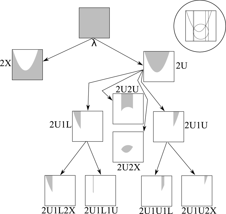
Figure 1: Depicted here is the Open NuCAD graph structure produced by the example run of TI-Open-NuCAD for input formula $F=[16y-16x^{2}-8x-1>0\wedge x^{2}+y^{2}-1>0]$. The leaf nodes are a weak decomposition of $\mathbb{R}^{2}$ into open cylindrical cells in which $F$ is truth-invariant. Also shown (circled) is the truth-invariant CAD for $F$.

Figure 1 shows the NuCAD tree resulting from the above execution of the TI-Open-NuCAD algorithm. There are seven leaf nodes, which mean $\mathbb{R}^{2}$ has been decomposed into seven cells. The standard truth-invariant CAD for input formula $F$ (shown circled in Figure 1) contains 16 open cells in $\mathbb{R}^{2}$. The Open NuCAD fails to be an Open CAD because the projections onto $\mathbb{R}^{1}$ of the cell $2X$ and any other leaf cell are neither disjoint nor identical.

The primary purpose of this example is to illustrate the basic functioning of TI-Open-NuCAD, and to illustrate the Open NuCAD data structure. Hopefully it has been successful in this. There are two important limitations to this example, though. First of all, Step 3, which deals with “fail” results returned by the OC-Merge-Set operation, is not illustrated. Secondly, and more importantly, because this example only involves two variables there is no opportunity to illustrate the reduction in the number and size of projection factor sets that we expect to accompany the model-based approach to CAD construction.

5 The correctness of TI-Open-NuCAD

In this section we sketch a proof of the correctness of TI-Open-NuCAD. In fact, TI-Open-NuCAD clearly meets its specification provided that Split meets its specification, and that termination can be proved. First we prove a lemma that is key to showing the termination of TI-Open-NuCAD.

For Open OneCell $D$ we denote the set of polynomials whose sections define the boundaries of $D$ by $\mbox{bpolys}(D)$ (note that they will be irreducible). For Tarski formula $F$ we denote the set of irreducible factors of polynomials appearing on the left-hand-side of the atomic formulas of $F$ when they are normalized to be of the form $f\ \sigma\ 0$ by $factors(F)$.

Lemma 1

Suppose the call $\mbox{Split}(D,F)$ produces a non-empty queue $Q^{\prime}$. Let $H$ be the closure under the Open McCallum projection of $\mbox{bpolys}(D)\cup factors(F)$. For each cell $C\in Q^{\prime}$, $\mbox{bpolys}(C)\subseteq H$.

Proof. First we note that if Step 2 produces $D^{\prime}=(\textsc{Fail},f)$ then although the sample point $\alpha$ and some of the algebraic numbers in the data-structure may change, the defining formula for $D^{\prime}$ and, therefore, the elements of $\mbox{bpolys}(D)$ remain the same. Next we note that if Step 2 produces a cell $D^{\prime}$ (i.e. does not produce Fail) then the specification of the O-P-Merge algorithm from [1], and by extension the OC-Merge-Set algorithm called in Step 2, guarantees that $\mbox{bpolys}(D^{\prime})$ is a subset of the closure under the Open McCallum projection of $\mbox{bpolys}(D)\cup Q$. Since $Q\subseteq factors(F)$, we have $\mbox{bpolys}(D^{\prime})\subseteq H$. For any cell $C$ enqueued on the output queue, at each level $i$, the boundaries of $C$ are sections of polynomials from the set $\{D[i].l,D^{\prime}[i].l,D^{\prime}[i].u,D[i].u\}$, which is a subset of $H$.          

Lemma 2

The Algorithm $\mbox{Split}(D,F)$ terminates and meets its specification.

Proof. As long as Step 3 only produces new values for point $\alpha$ that are in the cell defined by $D$ and Step 2 eventually produces a non-Fail result, $\mbox{Split}(D,F)$ clearly meets it specification. Moreover, if the body of Step 3 is executed and $\alpha$ is in the cell defined by $D$ (which is certainly true initially), then the new value of $\alpha$ is also in the cell defined by $D$. This is clear because $\gamma_{i}$ is chosen from the interval $(\mbox{max}(\zeta,D[i].L),\alpha_{i})\subset(D[i].L,D[i].U)$, and for $j\in\{i+1,\ldots,n\}$, $\gamma_{j}$ is chosen specifically to satisfy the defining formula

$$root(D[j].l,D[j].L.j,x_{j})<x_{j}<root(D[j].u,D[j].U.j,x_{j}).$$

What remains to be proven is termination, which boils down to showing that the call to OC-Merge-Set in Step 2 eventually returns a non-Fail result. If we were assured that OC-Merge-Set would produce the same projection factors for the perturbed $\alpha$ as for the original, this would be clear. Unfortunately, we cannot be sure of that. Thus, we require a more subtle argument. First, we note that each perturbation leaves the $x_{k}$th coordinate unchanged for all $k<i$, reduces the $i$th coordinates $\alpha_{i}$ so that it changes from a root of $g(\alpha_{1},\ldots,\alpha_{i-1},x_{i})$ to something slightly smaller (Step 3c), and potentially changes the remaining coordinates.

Suppose Split does not terminate. Then there is an infinite sequence of $\alpha$ values and associated $f$’s satisfying $f(\alpha)=0$. Note that all the polynomials $f$ as well as all the elements of the set $L$ constructed from $F$ come from the closure under the McCallum projection of $\mbox{bpolys}(D)\cup\mbox{factors}(F)$, which we’ll denote $P_{MC}$. Let $\alpha^{(0)},\alpha^{(1)},\ldots$ be the infinite sequence of values for $\alpha$ as the process progresses, let $f^{(0)},f^{(1)},\ldots$ be the infinite sequence of associated $f$’s and $L^{(0)},L^{(1)},\ldots$ and $i^{(0)},i^{(1)},\ldots$ be the associated values for $L$ and $i$ arrived at by Step 3b. We note that for any $k$, the elements $L^{(k)}$ all divide $A(i^{(k)},\alpha^{(k)})$, where

$$A(m,\rho)=\prod_{g\in P_{MC}|level(g)=m\wedge g(\rho_{1},\ldots,\rho_{m-1},x_{m})\neq 0}g.$$

We also note that the polynomial set $\{A(m,\rho)|m\in\{1,\ldots,n\}\wedge\rho\in\mathbb{R}^{n}\}$ is finite. So, for each $k$ we have that that $i^{(k)}$th coordinate of $\alpha^{(k)}$ is a zero of some $g\in L^{(k)}$ that is not nullified at $(\alpha_{1}^{(k)},\ldots,\alpha_{i^{(k)}-1}^{(k)})$ and thus is a zero of $A(i^{(k)},\alpha^{(k)})$.

We will show that for each level $r$, there is a value $k$ after which the $r$th coordinate of $\alpha^{(k)}$ never changes. We proceed by induction on $r$.

Consider the case $r=1$. Consider the subsequence $k_{1},k_{2},\ldots$ of all indices $k$ for which $i^{(k)}=1$. For each $k_{j}$ in this subsequence, $\alpha_{1}^{(k_{j})}$ is a zero of $A(1,\alpha^{(k_{j})})$. Moreover, the new value of $\alpha_{1}$ is smaller than the previous value and, since the value of the 1st component of $\alpha$ is otherwise never changed, $\alpha_{1}^{(k)}$ is strictly decreasing over the subsequence $k_{1},k_{2},\ldots$. Since $A(1,\beta)$ is the same for any $\beta\in\mathbb{R}^{n}$, and it has finitely many roots, there are only finitely many elements of the subsequence. In particular, there is a largest index $k^{*}$ in the subsequence ($k^{*}$ can be taken as zero if the subsequence is empty), and $\alpha_{1}$ is constant over all indices greater than $k^{*}$.

Suppose $r>1$. Assume, by induction, that the result holds for all smaller values of $r$. Then there is an index $k^{\prime}$ such that for all $k>k^{\prime}$ the first $r-1$ components of $\alpha^{(k)}$ are constant. So, for all $k>k^{\prime}$, the $r$th component of $\alpha^{(k)}$ is non-increasing. Consider the subsequence $k_{1},k_{2},\ldots$ of all indices $k>k^{\prime}$ for which $i^{(k)}=r$. Note that because the $r$th component of $\alpha$ is reduced at each step for which $i^{(k)}=r$, the sequence of values $\alpha_{r}^{(k_{1})},\alpha_{r}^{(k_{2})},\ldots$ is strictly decreasing. For each $k_{j}$ in the subsequence, $\alpha_{1}^{(k_{j})}$ is a zero of $A(r,\alpha^{(k_{j})})$. Since there are only finitely many polynomials $A(r,\beta)$, where $\beta\in(\alpha_{1}^{(k^{\prime}+1)},\ldots,\alpha_{r-1}^{(k^{\prime}+1)})\times\mathbb{R}^{n-r+1}$, each having only finitely many roots, there are only finitely many elements in the subsequence. In particular, there is a largest index $k^{*}$ in the subsequence ($k^{*}$ can be taken as $k^{\prime}$ if the subsequence is empty), and $\alpha_{r}$ is constant over all indices larger than $k^{*}$.

Thus, we have proven that there is an index $k^{\prime}$ such that for all $k>k^{\prime}$, all coordinates of $\alpha^{(k)}$ are constant. This is a contradiction, since executing Step 3 changes $\alpha$, which means that our assumption that there is an input for which Split does not terminate is invalid. This completes our proof of the termination and correctness of Split.          

Theorem 2

Algorithm TI-Open-NuCAD terminates, and meets its specification.

Proof. Lemma 2 shows that Split terminates and is correct. Lemma 1 shows that the boundary polynomials for the cells returned by Split are elements of the closure under the Open McCallum projection of $\mbox{factors}(F)$. Thus for any cell $D^{\prime}$ returned by Split, and any cell $C$ from the CAD produced by the Open McCallum projection for $F$, either $C\cap D^{\prime}=\emptyset$ or $C\subseteq D^{\prime}$. This means that for each each cell $D$ enqueued on $Q$, we can imagine associating with $D$ the set of cells from the CAD produced by the Open McCallum projection for $F$ that are contained in $D$ — we call this set $M_{D}$. Note that $M_{D}$ is never empty. Recall that when a cell with label ending in $X$ is dequeued from $Q$, no call to Split is made. Define $X_{Q}$ to be the set of cells in $Q$ with label ending in $X$. Consider the quantity

$$c_{Q}=|X_{Q}|+\sum_{E\in Q-X_{Q}}2|M_{E}|^{2}.$$ (2)

We will show that at each iteration of the loop in Step 4 of TI-Open-NuCAD the quantity $c_{Q}$ is reduced. Every iteration, a cell $D$ is dequeued from $Q$ and one of the following occurs:

1. no new cells are enqueued — in which case one of the terms on the right-hand side of (2) gets smaller and the other term is unchanged,

2. a single cell whose label ends in $X$ is enqueued — in which case $|X_{Q}|$ increases by one, but $\sum_{E\in Q-X_{Q}}2|M_{E}|^{2}$ is reduced by $2|M_{D}|^{2}>1$ ,

3. more than one cell is enqueued — in which case the $|X_{Q}|$ term is increased by one, but in the sum the term $2|M_{D}|^{2}$ is replaced by $2|M_{D_{1}}|^{2}+2|M_{D_{2}}|^{2}+\cdots+2|M_{D_{t}}|^{2}$ where $|M_{D}|=|M_{D_{1}}|+|M_{D_{2}}|+\cdots+|M_{D_{t}}|$, $t\geq 2$. So the net change is

   $$1+2|M_{D_{1}}|^{2}+2|M_{D_{2}}|^{2}+\cdots+2|M_{D_{t}}|^{2}-2|M_{D}|^{2}<0.$$

Thus, termination is proven and, as noted previously, correctness is then easily verified.          

6 Advantages of the model-based approach

Further work is required to either produce an implementation of these algorithms and provide a systematic empirical comparison between them and the usual Open CAD construction algorithm, or to provide an analytical comparison. Moreover, in as much as an Open NuCAD is less structured than an Open CAD, it cannot necessarily be used for the same purposes. So yet more work is required to understand the applications and limitations of this new variant of CAD. Given these points, it is worth listing some of the reasons why the model-based approach and Open NuCADs are important and worth developing.

1. The model-based approach produces smaller projection-factor sets and larger sign-invariant cells. This point is demonstrated in [1], and further experiments showing this were presented in the ISSAC 2013 talk accompanying that paper. This is perhaps the most important reason to pursue this new approach, because the reduction in the number of projection factors and the increase in cell size is substantial. For a single cell, experiments point to exponentially smaller projection factor sets and exponentially larger cells.

2. NuCADs allow for truth-invariant decompositions for an input formula using fewer cells than CADs. The example in this paper demonstrates this point, although certainly more analysis, either empirical or analytical, is required to understand how substantial the difference between NuCADs and CADs really is.

3. Model-based construction of NuCADs is incremental. After one loop iteration, which requires a small amount of time and space relative to even just the projection step for CAD construction, the new approach produces a cell in which the input formula is truth-invariant. This is in marked contrast with traditional CAD construction, for which the entire projection must be computed before even the first cell is constructed.

4. Model-based construction of NuCADs is naturally parallelizable. Splitting of one cell in the queue $Q$ is completely independent of splitting other cells, so all the splitting can be done in parallel. In fact, nodes could keep their own queues of cells to split, and would only need to communicate when one node ran out of cells to split and had to steal some from another’s queue. The one kind of information that one would probably want nodes to share would be the results of particularly expensive resultant and discriminant computations and the accompanying factorizations.

Perhaps the most interesting of all, however, is that none of the proofs of the doubly-exponential worst-case running time of CAD apply to NuCADs. [2, 3, 5] all deduce the doubly-exponential worst-case performance of CAD from its connection to quantifier elimination — in particular, quantifier elimination for formulas with many quantifier alternations. NuCADs, however, do not directly allow for quantifier elimination, at least not for formulas with quantifier alternations, so they are not subject to that argument. This leaves open the intriguing possibility that the model-based approach and NuCADs may provide a CAD-style algorithm for satisfiability, existential quantifier elimination, or even full quantifier elimination with an asymptotic complexity competitive with modern QE algorithms, but with the kind of practical utility that has made CAD attractive for smaller problems.

References

- [1] Christopher W. Brown. Constructing a single open cell in a cylindrical algebraic decomposition. In Proceedings of the 38th international symposium on International symposium on symbolic and algebraic computation, ISSAC ’13, pages 133–140, New York, NY, USA, 2013. ACM.
- [2] Christopher W. Brown and James H. Davenport. The complexity of quantifier elimination and cylindrical algebraic decomposition. In ISSAC ’07: Proceedings of the 2007 international symposium on Symbolic and algebraic computation, pages 54–60, New York, NY, USA, 2007. ACM.
- [3] J. H. Davenport and J. Heintz. Real quantifier elimination is doubly exponential. Journal of Symbolic Computation, 5:29–35, 1997.
- [4] Dejan Jovanović and Leonardo de Moura. Solving Non-linear Arithmetic. In Bernhard Gramlich, Dale Miller, and Uli Sattler, editors, Automated Reasoning, volume 7364 of Lecture Notes in Computer Science, pages 339–354. Springer Berlin Heidelberg, 2012.
- [5] V. Weispfenning. The complexity of linear problems in fields. Journal of Symbolic Computation, 5:3–27, 1988.