Credit acceptance process strategy case studies - the power of Credit Scoring

Abstract

The paper is aware of the importance of certain figures that are essential to an understanding of Credit Scoring models in credit acceptance process optimization, namely if the power of discrimination measured by Gini value is increased by 5% then the profit of the process can be increased monthly by about 1 500 kPLN (300 kGBP, 500 kUSD, 350 kEUR). Simple business models of credit loans are also presented: acquisition - installment loan (low price) and cross-sell - cash loans (high price). Scoring models are used to optimize process, to become profitable. Various acceptance strategies with different cut-offs are presented, some are profitable and some are not. Moreover, in a time of prosperity some are preferable whilst the inverse is true during a period of high risk or crisis. To optimize the process four models are employed: three risk models, to predict the probability of default and one typical propensity model to predict the probability of response. It is a simple but very important example of the Customer Lifetime Value (CLTV or CLV) model business, where risk and response models are working together to become a profitable process.

Key words: credit scoring, crisis analysis, banking data generator, retail

portfolio, scorecard building, predictive modeling, credit acceptance process.

1 Introduction

In this paper some typical predictive models called Credit Scoring models or scorecards (Thomas et al., 2002; Anderson, 2007) are considered. These models are created based on logistic regression, especially the most known WoE approach (Siddiqi, 2005). Their construction is very simple and useful in interpretation, so they have become the best tools in the optimization of processes in many financial institutions. For example, they are used in banking (Huang, 2007) to optimize credit acceptance processes and in PD models (probability of default) in regulator recommendations Basel II/III to calculate RWA (Risk Weighted Assets) (BIS-BASEL, 2005).

Credit Scoring models are examples of statistical predictive models for forecasting some events based on collected and available data history. The best way to gauge their value is to wait and test them on real data, or, in other words, to compare the predicted values with observed. Unfortunately, this can take a considerable amount of time. To test the whole process, including the steps necessary in legal collection, can take between 5 and 10 years.

Credit Scoring research as a typical applied statistics field is fully connected with data science and with studies on real data taken from business banking processes. Legal constraints and lack of perspective thinking among data owners can result in very real problems connected to access to real data and almost totally blocks any correctly led research. A change in thinking has occurred in biostatistics where access to real data is now possible, profiting both data scientists and data owners. Even sometimes data are taken from the reality, however, in most cases they are insufficient to provide the complex analyses which are expected.

In the very interesting new paper presented at the conference Credit Scoring and Credit Control XIII in Edinburgh (Lessmanna et al., 2013) all the available data used in the last ten years are presented. Many of them are used only once in order to highlight particular results. Only a few of them can be accessed by the public, but only one dataset has more than twenty variables and another with more than 150k observations. Based on this information it becomes clear that there is a need for new simulated data for the Credit Scoring analyses described by (Kennedy et al., 2011).

Let a set of simulated data be considered. All the rules used for data creating are known. Even if the Monte Carlo simulation, which is based on random numbers, is used repeatedly, all the final numbers are totally deterministic and can be repeated once again with the same number sequences. The following conclusion can, as a result, be reached: that research using this kind of data is ultimately futile, because all the previously held rules confirm only the method of data simulating. It is not true, because the method of data creating are completely different than scoring techniques, so it is nontrivial problem to find out description of the data based on scoring models. Moreover simulated data have many properties not planed and quite interesting. Complexity of the process is too hard to imagine and explain all unexpected behaviour, so also the author of the data can be surprised. There is needed a deeply study to point out total secret structures of new simulated data.

All the above mentioned arguments lead us to focus on simulated data. Furthermore, they also go so far as to suggest a change to a paradigm in applied statistics. Namely there is no requirement to always commence scientific research from the point of access to data. Maybe the question should be formulated as: what data are needed to ensure control of the process being studied in order to predict the future indicators? It can be extremely risky to believe that real data can be sufficient. Observed data does not show latent variables. Simply because it has been observed does not mean that it is possible to explain. It should always be remembered that there is a necessity to focus on the hidden or latent information. It is for this reason that simulated data can be very useful, because invisible numbers, for example, risk measures calculated on rejected applications that are unobservable in reality, can be presented. This is a very valuable rule created by Total Quality Management (TQM) suggesting that decisions should be made on both: visible and invisible numbers.

The need of creating simulated data can also be described in the following way: in the typical credit acceptance process reports are made known such as decline reasons, vintage, flow-rates, profile customer evaluation in the time, segmentations etc. All these reports are the results of observed information. The question what part do the hidden processes play in these results, could be considered.

2 Simulated data creating, instalment loans case

Consumer finance data generator in the first form is described by (Przanowski, 2013). It is dataset dedicated to only one product: an instalment loan. Every client has only one loan. All variables therefore are based only on one account history. The Markov chain and fixed transition matrix with calculated migration coefficients between states defined as a number of delinquent instalments per month is used. For every month on every account dedicated scoring connected with all available history up to current month is calculated. Every succeeding month of data is calculated based on the mentioned matrix and scorings. If an account score is low then in the next month the account under consideration has some due instalments dependent on the scoring bracket, the score belongs to better brackets, then the account remains in the current state or goes into a non-delinquent state.

Dataset contains 2 694 377 rows and 56 columns.

3 Credit acceptance process profitability, predictive power impact

It is obvious that Credit Scoring models are used in banking processes in the optimization purpose. It cannot be questioned, but up to now there have been no direct numbers about the usefulness of scorings presented in references, or about the profit values dependent on the scoring discrimination powers. This is probably due to the secret know how of enterprises. This is why random simulated data can be useful. The case under consideration is not connected with any secret bank indicators, but, on the other hand, some estimated, relatively realistic numbers to imagine the power of scoring models and the main, key success factor in the banking business.

The source simulated data are specially changed to have a global risk, on all rows, at the level of 47%. Following this, a few scoring models are constructed with different discrimination powers measured by Gini statistics (Siddiqi, 2005).

It is not possible to present detailed Profit&Loss (P&L) report without knowledge about certain specific factors connected to the business field and market, but it is sufficient to focus on the main dimensions: incomes coming from interest rates and provisions; and losses calculated by Basel II/III recommendations as an expected loss.

The following definitions are necessary to understand profit notion: ${\rm APR}$ - annual percentage rate for credit loans, $r={{\rm APR}\over 12}$, $p$ - provision for credit granting paid at the beginning, $A_{i}$ - loan amount, $N_{i}$ - number of instalments, where $i$ is index, account ID. Based on current Basel recommendations expected loss (EL) is defined as a multiplication of three factors: probability of default (PD), loss given default (LGD) and exposure at default (EAD). Without any special argumentations, using a conservative approach it can be assumed that: LGD=50% and EAD is the loan amount. Based on historical data, where default events are available, PD can be transformed from expected value into an observed one, namely when a default event is present (it can be written as ${\rm default}_{12}={\rm BAD}$) then PD=100% and where the opposite is the case PD=0%. In this case the observed loss $L_{i}$ is calculated. Incomes $I_{i}$ including provisions are calculated based on compound interest (geometric series). For every $i$ - account:

$$L_{i}=\left\{\begin{array}[]{ll}50\%A_{i},&\textrm{\rm when default}_{12}={\rm BAD},\\ 0,&\textrm{\rm when default}_{12}\neq{\rm BAD}.\end{array}\right.$$

$$I_{i}=\left\{\begin{array}[]{ll}A_{i}p,&\textrm{\rm when default}_{12}={\rm BAD},\\ A_{i}\left(N_{i}r{(1+r)^{N_{i}}\over(1+r)^{N_{i}}-1}+(p-1)\right),&\textrm{\rm when default}_{12}\neq{\rm BAD}.\end{array}\right.$$

The total profit $P$ can be calculated as follows:

$$P= \sum_{i}I_{i}-L_{i}.$$ (3.1)

For every scoring model, with different predictive powers, all the applications can be sorted using score values from the worst, with the highest risk, to the best, with the lowest risk. Based on the cut-off parameter any profit can be calculated on an accepted part and acceptance rate. Repeating that procedure many times for all possible cut-offs and all scoring models defined profit curves are constructed. These are presented in figure 1. Note that all numbers on pictures are presented in PLN, but some important indicators are also recalculated in GBP, USD and EUR. Some of them, for Gini this is usually lower than 50%, never produce profits, for any acceptance rate the total profit is always negative. Based on this, any scoring models with a low power or a low power of all acceptance rules, is not possible to manage the business and be profitable. Moreover, for a scenario when all the accepted applications are present, the profit is likely to be negative: a level of -44,5 mPLN (-9 mGBP, -15 mUSD, -10 mEUR).

The best three curves, with possible profitable scenarios, are presented on figure 2. Scoring models with a power greater than about 50% are able to identify profitable subsets of applications. The better the power, the greater the acceptance rate and profit. In the case of a scoring model with a power of 89%, which is too high to be realistically entertained, can be accepted about 44% of all applications resulting the total profit 10,5 mPLN (2 mGBP, 3.5 mUSD, 2.5 mEUR). These numbers are essential to understand the usage of scoring models. Dependent on the quality of the scoring model and its predictive power, a bank may lose or gain millions of currency units. Scoring is the key success factor in increasing capital for a company.

Profitability connected with correct usage of scoring models can also be presented in the following way. A calculation of the shift of profit and acceptance rate in the credit acceptance process when the increase of predictive power is equalled to 5%, can be seen in table 1. If Gini is increased by 5%, then the profit of the process can be increased monthly by about 1 500 kPLN (300 kGBP, 500 kUSD, 350 kEUR) the acceptance rate can be increased by 3,5%. Alternatively, when an increase of acceptance rate is unnecessary, then a bank may save money only through the use of the better scoring model. Namely, with an acceptance rate set at 20%, losses of approximately 900 kPLN (180 kGBP, 300 kUSD, 210 kEUR) can be saved. In the case of 40% approximately 1 500 kPLN (300 kGBP, 500 kUSD, 350 kEUR) can be saved monthly.

The large amounts of potential profits or saved losses that are here presented may help persuade banks and other financial institutions to retain analytical teams in their employment. They may also help simulate the search for better models and a recognition of the need to test any new model that appears. Finally, they acknowledge the importance of necessity of champion challengers and parallels acceptance scenarios.

The general message seems to indicate that providing the figures quoted above are correct, then any changes in the acceptance rate are influenced by Reject Inference (Huang, 2007). The inability to make correct risk estimations on rejected applications results in a substantially large bias in the profit estimation, so it is by no means straightforward to manage the credit acceptance process. Section 6 deals with it in detail.

Table 1: Shifts for finance indicators dependent on predictive power change.

Indicator	Value
Number of credit applications per month	50 000
Average loan amount	5 000 PLN (1 kGBP, 1.6 kUSD, 1.1 kEUR)
Average number of instalments	36 months
Annual percentage rate	12%
Provision for loan granting	6%
Global portfolio risk	47%
Increase of predictive power	5%
Increase of acceptance rate	3,5%
Increase of monthly profit	1 500 kPLN (300 kGBP, 500 kUSD, 350 kEUR)
Decrease of monthly loss (AR=20%)	900 kPLN (180 kGBP, 300 kUSD, 210 kEUR)
Decrease of monthly loss (AR=40%)	1 500 kPLN (300 kGBP, 500 kUSD, 350 kEUR)

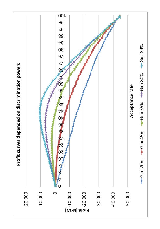
Figure 1: Profit curves.

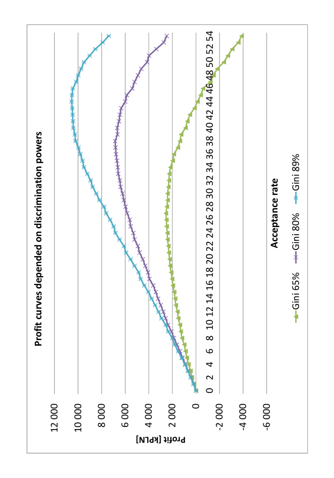
Figure 2: The three best profit curves.

4 Business model: acquisition and cross-sell

The last crisis (between 2008 and 2009) was a period when risk on some credit products, especially cash and revolving loans, dramatically increased. Consequently, many banks decided to decrease production, e.g. acceptance rates, to stabilize risk, trying to not exceed loss values and so become non-profitable. Currently, banks, in the hope that the crisis has passed, have observed very low risk in their portfolios. There are some cases where this is actually lower than prior to the crisis. Consequently, many have taken the decision to increase acceptance rates. In the current climate this has led to a struggle to attract customers. Because the observed risk is presently relatively low, some customers segments are not profitable. In the case where a customer does not want to take a loan credit, the bank is attempting to attract them by minimizing the price (e.g. APR or provision). This sometimes results in no profit gain. A customer desperate for a loan is, in most cases, an extremely risky proposition. The fight is on to find customers with the right level of risk. In order to retain business, banks have to find a balance between profitable and overly risky customers.

The above results in the development or improvement of two-stage business models: the low and attractive model or the null price acquisition model, when a customer is started to establish an emotional relation with our bank, and then provide him many expensive repeat business products, cross-sell.

One of the most well-known two-stage business models in banking is: instalment loan as an acquisition and cash loan as a cross-sell. A Customer purchasing a TV-plasma in a store in small instalments is usually quite satisfied with the arrangement. During the loan cycle the customer gets many cross-sell contacts or offers of cash loans. Some customers decide to purchase a further product and a subset of them are transformed into regular cash loan taking customers a very profitable segment. Even if the business model is known it is not easy to manage it and to maximize a profits. This is the best example of where the importance of Credit Scoring Models can be illustrated.

Simulated data are also very useful in cut-off calculations. It is incorrect thinking to separate model building from its implementation. These two steps are always connected and Credit Scoring research cannot be focused only on various building techniques studies. When we want to build good models we need to test them in real production. Sometimes production results are quite different from those that are expected and an in-depth analysis of this difference is essential in the model building process.

It is an observed fact that future risk and instalment payments are correlated with available historical data on the customer. We can say that the customer’s current ability to pay the next set of instalments is largely dependent upon their previous performance of repayments as well as upon their current financial, employment, home and domestic situation. The customer also has their own priorities in loan repayments; some are paid regularly and some are paid before the due date; sometimes repayments are not made. These priorities are in some part connected with banks processes and collaterals, but the simplest way is to assume that any loan that is taken out alongside another loan will only serve to increase risk. Every customer has an ideal number of loans that they are able to successfully manage, but if the bank allows them to exceed this number, the customer may well default on repayments.

Let us consider one customer with applications for more than one loan. A bank may choose to grant all of them or only a part. As mentioned previously, the repayment of any successive loan is dependent on the history of previous repayments, but on only accepted and financed loans. It is not possible to consider all scenarios and to build model data in that case, but very simple solution is to assume that every application is somewhere accepted and then financed. When the customer applies for a loan for the first time he usually tries to get it from his favourite bank. If his application is rejected, he is likely to approach another bank, but if this application is turned down, then he may approach another type of financial institution or an individual. We can assume that loans are always granted, but not always by the same bank. We can also use the basic economists thesis that expenses are not correlated with incomes. The same may be applied in the case of the granting of loans. The customer takes out a loan for his own individual reasons though these may not be connected to his affordability.

Let the basic assumptions of random data generator for Consumer Finance business model be formulated (acquisition = instalment loans and cross-sell = cash loans):

• The customer can only take out two types of loan: an instalment loan to purchase goods and a cash loan for any other purpose

• Instalments loans are low risk and are not dependent on historical cash loans taken by the same customers

• Cash loans are high risk and are dependent on the individual’s repayment history: instalment and cash loans

• The most risky loan for a customer is the last loan from any outstanding loans

• A cash loan can be granted in a particular month only when in the previous month a customer had some active accounts. In other words, every cash application is linked to publicity material dealing with offers that are only available to the bank’s customers

• In any month there can only be one of two events: payment of several instalments or null payment, in databases information is collected regarding paid and due instalments

• The distributions of characteristics are precisely defined using expert knowledge and are based on various random generators

• If a customer has 7 due instalments on his account (180 past due days), then the account is closed with the status B (Bad) and history is not produced for any succeeding months

• If all payments are made, then account is given a status C (closed correctly) and the history of that account is discontinued

• Payments or non-payments are dependent on three factors: score value calculated on account and customer level (there are about 200 characteristics), transition matrix and macro-economic variable that changes the matrix over time.

All data are created on laptop Dell Latitude (1,67 GHz). Time of processing: 15 hours.

Datasets for instalment loans: Production dataset - 56 335 rows and 20 columns. Transaction dataset - 1 040 807 rows and 8 columns. All months are presented in figure 3, where ${\rm default}_{3}$, ${\rm default}_{6}$, ${\rm default}_{9}$ and ${\rm default}_{12}$ means shares of accounts with 90+ past due days, three due instalments (in case ${\rm default}_{3}$ exceptionally 60+, two due instalments).

Datasets for instalment loans: Production dataset - 60 222 rows and 19 columns. Transaction dataset - 1 023 716 rows and 8 columns. All relevant months are presented in figure 4. Additionally, the time period is divided into two periods: 1975-1987 - modelling dataset, where all parameters are calculated and 1988-1998 for testing.

Stock months are presented in figure 5. The response rate equalled to about 5% calculated as the number of total cash applications in the following month over the total number of active accounts in the potential market in the current month is also presented.

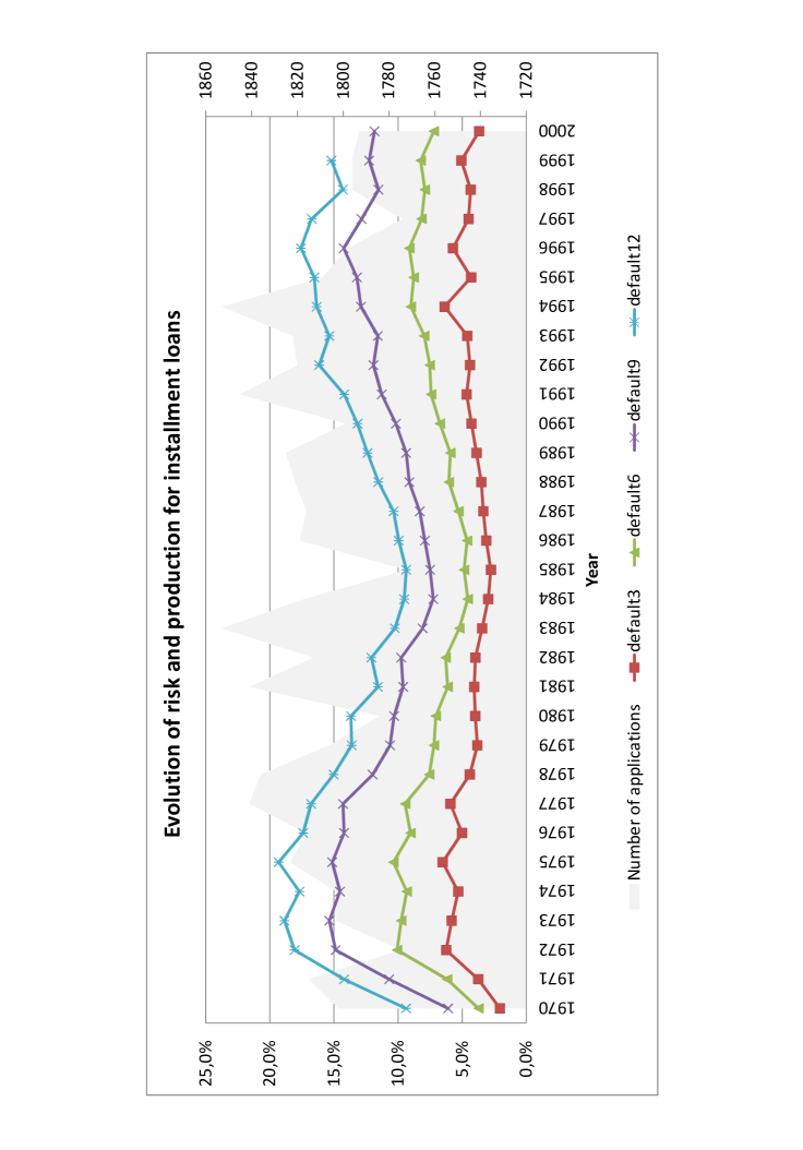
Figure 3: Instalment loan.

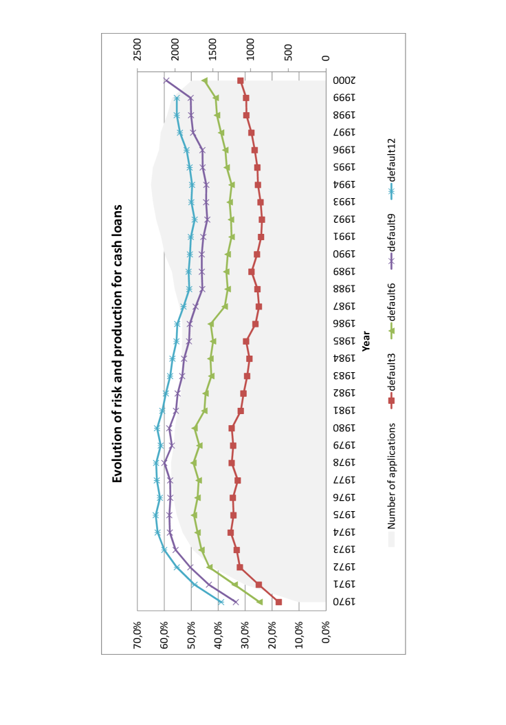
Figure 4: Cash loan.

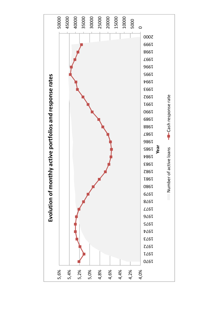
Figure 5: Stock months.

5 Basic parameters calculation

All the simulated data, instalments and cash loans are available for a bank, allowing them the potential to expand on their role in the market. The customer has his own priority regarding repayments, some of their liabilities are prioritised; others are not. A bank can define a proper policy and set of acceptance rules to minimize any loss. Optimization is possible due to scoring models implemented in the decision engine, a specially dedicated IT tool for automatic processing. The bank can only optimize risk by its decisions: to accept or reject a particular applied request. Acceptance implies inserting the whole generated history of processed application into bank’s portfolio. It is assumed that all the account history is calculated before and is unchanging, so the issue is only to make a correct decision at the moment of the application based solely on any available customer history up to date of application. If a decision is negative then the bank does not have the history of that account in its portfolio.

The bank, depending upon its decision, has either a better or poorer knowledge of its customers. This poses an interesting question, which is better? To have available all information about a customer, about all his loan histories, but have a greater loss, or to have less information with lower a loss. Every rejected application of a particular customer results in a worse estimation of risk for future loans of that customer. The sample in the bank’s portfolio of that customer is biased. The problem is called Reject Inference and today is described in many works (Huang, 2007; Anderson et al., 2009; Hand and Henley, 1994; Verstraeten and den Poel, 2005; Finlay, 2010; Banasik and Crook, 2003, 2005, 2007). The bank cannot avoid the above-mentioned problem, it can only minimize it or get more data from credit bureau companies. If the credit bureau in the country is managed properly and has all loans available in the market, then that information can be very useful in minimizing reject inference.

When bank knows more about his customers then it is able to estimate any potential risk in a better way, so it is able to provide its business a more stable and safer manner.

Four models are constructed: three risk models and one response model. All the models are built on the same sample time period 1976-1987:

• PD Ins - PD model to predict probability of instalment ${\rm default}_{12}$.

• PD Css - PD model to predict probability of cash ${\rm default}_{12}$.

• Cross PD Css - PD model to predict probability of future cash ${\rm default}_{12}$ at the time of instalment application.

• PR Css - response model to predict probability of future cash response at the time of instalment application.

Model documentations are presented in 8.2.

The main goal is to make the process profitable and to maximize profit. Simple factors are calculated: income - interest rate incomes and loss - expected loss based on known Basel formula: EL=PD*LGD*EAD see also formula 3.1. Parameters are set as follows:

The annual percentage rate (APR) for an instalment loan is $1\%$, APR for cash loans $18\%$. Average LGD values: $45\%$ for instalment and $55\%$ for cash loans. PD for EL formula is binary variable ${\rm default}_{12}$. To simplify the cross-sell process all cash loans are the same: loan amount $5000$PLN and the number of instalments - $24$.

Financial KPIs for the modelling period 1975-1987 are presented in table 2. Table 3 provides predictive the powers of built and used models, some powers are not realistic, especially for the response model, but that case represents a strategy of full acceptance in $100\%$, which is a fairly unreal scenario and is considered only due to random data. It is useful to study it, because we can observe a case without any reject inference.

Table 2: Finance KPIs for global process, where all applications are accepted (period 1975-1987).

KPI	Instalment	Cash	All
Profit	-7 824 395	-31 627 311	-39 451 706
Income	969 743	10 260 689	11 230 432
Loss	8 794 138	41 888 000	50 682 138

Table 3: Predictive powers (period 1975-1987).

Model	Gini
Cross PD Css	74,01%
PD Css	74,21%
PD Ins	73,11%
PR Css	86,37%

The average risk value of this process is 37,19% and the average probability (PD) - 34,51%, so the expected value is slightly underestimated. The global profit is negative about -40 mPLN. The chance of making a profit is understandably not a straightforward task. However, a solution can be found that is based upon the Customer Lifetime Value (CLTV, or CLV) modelling methods (Ogden, 2009; DeBONIS et al., 2002). It uses a relatively simple version that is based upon one response three risk models.

The goal of maximizing profit can be achieved by finding proper cut-offs for the above-mentioned four models. We should also be aware of the general idea of processing. All customers and their loans with all relevant history are collected in a database that we can call portfolio potential. Our decision engine can only accept or reject loans. If some applications are rejected then some missing information about our customers is present. That missing one has an effect on risk expected values, on score distributions and on the ABT variables distributions described in section 8.1. So on the one hand our bank can have lower risk, because some applications are rejected, but on the other some important information about customers is lost. Moreover, if some loans are not accepted, there may be some other type of value missing present, namely when a cash loan is being taken out. If we do not have a customer with active loans in our portfolio, we are not able to send them cash offers, so we do not know, or rather the customer does not know, they may access to cash in our bank, so we end up losing that customer. That kind of missing information in acceptance strategies is indicated as ’not known customer’.

First we try to optimize all cash loans. Based on a simple profit curve a proper cut-off on PD Css probability values can be found, namely with an acceptance rate of 18,97% we have the best profit = 1 591 633 PLN. In the decision engine we introduce the rule: when $PD\_Css>27,24\%$ then reject.

Following CLTV methodology the sequence of cash loans should be considered which would then be analysed in a more efficient manner to discover the final profit. This exercise is studied only in the case when the first product is an instalment loan. Also considered is the future cash loan for the same customer. Of course, not every customer taking out an instalment loan is taking cash later. Only some of decide to take cash, so some customers, especially those with only instalment loans, are rather non-profit. Our process should be focused on customers with a bigger chance for future cash loan, because only from that kind of customer we can earn money.

Based on models PD Ins and PR Css five (from 0 to 4) segments are created separately. The first, early discovered rule is also considered. For every combination of groups the global profit is calculated taking into account the currently applied instalment loan and future cash loan (see table 4). Based on that table new rules are defined:

• when $PD\_Ins>8,19\%$, then reject

• when $8,19\%>=PD\_Ins>2,18\%$ and $(PR\_Css<2,8\%$ or
  $Cross\_PD\_Css>27,24\%)$, then reject.

It should be emphasized, that the last rule is based not only on risk parameters. It can be interpreted in the following way: if a customer takes only an instalment loan, then the cut-off can be set on a different level than for customers who take cash loans in the future.

All the defined rules should result in 1 686 684 PLN of global profit. If the last rule is omitted, that is with only one acceptance rule: $PD\_Ins\leq 8,19\%$, then the global profit will be 1 212 261 PLN. So we will lose about 470 kPLN, which will be about 30% lower profit.

Unfortunately, the numbers and ideas presented are biased by Reject Inference. To be sure of the final numbers we need to run the acceptance process, calculate once again all the ABT variables, based on new decisions, and then we will be able to get the proper financial KPIs. This is the reason for the various strategy testing in section 6.

The method presented for cut-offs calculation is only an example and can be treated as a nice exercise to learn the complex processes and correlations between many factors. In the real-life situation more correctly defined goals, boundaries, constraints or restrictions should be considered. Nevertheless, the technique is always the same; all the possible scenarios are considered. Only then are the KPIs calculated and the best solution is decided upon. But the problem of reject inference is always present and it is not easy to consider its impact in an appropriate manner.

Table 4: Combinations of segments (groups) and their global profits (period 1975-1987).

GR PR	GR PD	Number	Global	Min	Max	Min	Max
Css	Ins	of Ins applications	profit	PR Css	PR Css	PD Ins	PD Ins
4	0	1 277	372 856	4,81%	96,61%	0,02%	2,18%
4	1	581	96 096	4,81%	96,61%	2,25%	4,61%
1	0	2 452	67 087	1,07%	1,07%	0,32%	2,18%
3	0	907	46 685	2,80%	4,07%	0,07%	2,18%
3	1	734	14 813	2,80%	4,07%	2,25%	4,61%
3	2	307	12 985	2,80%	4,07%	4,76%	7,95%
4	2	361	8 039	4,81%	96,25%	4,76%	7,95%
3	3	446	-1 283	2,80%	4,07%	8,19%	18,02%
4	3	417	-5 774	4,81%	95,57%	8,19%	18,02%
1	1	3 570	-82 886	1,07%	1,07%	2,25%	4,61%
1	2	4 044	-408 644	1,07%	1,07%	4,76%	7,95%
3	4	726	-946 937	2,80%	4,07%	18,50%	99,62%
4	4	1 054	-1 108 313	4,81%	96,25%	18,50%	99,83%
1	3	3 883	-1 270 930	1,07%	1,07%	8,19%	18,02%
1	4	2 878	-4 306 859	1,07%	1,07%	18,50%	97,00%

6 Various strategies study

To understand the complexity of the process four acceptance strategies are presented, see tables 5, 6, 7 and 8.

The first strategy is connected to the cut-offs calculation approach mentioned in section 5. Let we us remember that in the period 1975-1987 the expected total profit is 1 686 684 PLN. After running the process we arrive at 663 327 PLN. There is an error of approximately one million PLN. What is going on? Where is our money? The error is very significant and it is because of rejected applications, 30% of share, and due to not known customer decline reasons, 50% of share. On the other hand, we can content ourselves in the knowledge that our profit is still positive by about 700 kPLN, as opposed to the total acceptance strategy with a negative profit equalling -40 mPLN. Despite this small success the error is too significant to ignore, it persuades us to study further and broaden our minds in order to be aware that building models with large predictive powers is not enough to win an implementation step. Taking into account all the factors and all the steps is also very important.

To be very honest, nobody can guarantee a success in any case where the strategy is dramatically changed. Let we emphasize that the initial strategy is based on the fully acceptance process, so from a 100% acceptance rate is switched to 26% on instalment loans and 16% on cash. Such a radical step plays a profound part in the distributions of our probabilities. To begin with, PD is at a level of 34,51%. In the new process we have 28,87%. Why do we have a difference? It is due to missing information about all of the customer’s accounts. The new strategy accepts less risky applications, so the bank has information only about better loans, so the average PD should be lower, which causes an underestimation of risk regarding our customers.

In the inverse case, based on first strategy, if we want to increase acceptance, we will be in trouble because we will have incorrectly estimated risks parameters. Moreover, we will realise that the properties of the models are also changed, and the predictive powers are lower. Gini of model Cross PD Css from 74% decreased up to 41% on all and to 21% on accepted segment. In reality, only the second value is observed, so we can discuss about the correctness of that model. Why does the model not work? It is really difficult to measure the value of that model after implementation. Probably it will be replaced by another one.

In section 5 the result is also shown in the case of one simple rule without any special rules based on response probabilities. In that case the expected profit is lower by about 470 kPLN. It falls by about 550 kPLN (see strategy 2, table 6), so in estimations of differences we do not have any significant errors.

We can formulate a simple rule: reject inference is difficult to predict, it is proportional to the strength of the acceptance process change. If we change a process significantly, we can also expect significant error in predictions due to rejected applications.

Let we consider another approach. Let’s start from a simple intuition strategy, where we do not accept applications with default events (more than three due instalments) during the last 12 months before the application date. The process is not profitable (see strategy 3, table 7), but acceptance of cash loans is decreased to 45%. The models still work in that case. Repeating the same idea as for cut-offs calculation for the first strategy, we can once again set new cut-offs, but in that case based on a different starting strategy. We have therefore created the next strategy (see strategy 4, table 8).

The profit is 732 kPLN, with 9% acceptance for cash and 26% for instalment loans. We can discuss this strategy further, it is a better solution for the period 1975-1987, but acceptance of cash loans is very small, which is only right for such a period of high risk. Indeed, in the period 1988-1998 we have the invers case: the first strategy has a profit of 1,5 mPLN but the forth a little bit lower 1,3 mPLN.

All the exercises presented give us the opportunity to understand complex problems and to be aware of reject inference in practice.

The most important conclusions are: because we are able to create useful data for Credit Scoring analysis, we can make many strategies, build various models, test CLTV approaches and develop better estimations of reject inference.

Table 5: Strategy 1.

Period	Income	Loss	Profit
1975-1987	3 407 745	2 744 418	663 327
1988-1998	3 761 299	2 246 844	1 514 455

Rule	Description
PD_Ins Cutoff	$PD\_Ins>8,19\%$
PD_Css Cutoff	$PD\_Css>27,24\%$
Special for PD and PR	$8,19\%>=PD\_Ins>2,18\%$ and $(PR\_Css<2,8\%$ or $Cross\_PD\_Css>27,24\%)$

Cash loan

Rule	Number of applications	% of applications	Loan amount	Risk	Profit
PD_Css Cutoff	8 436	32,97%	42 180 000	67,99%	-13 098 591
Not known customer	12 999	50,80%	64 995 000	65,91%	-19 171 357
Accepted	4 152	16,23%	20 760 000	22,35%	642 637
All	25 587	100,00%	127 935 000	59,53%	-31 627 311

Instalment loan

Rule	Number of applications	% of applications	Loan amount	Risk	Profit
PD_Ins Cutoff	9 289	39,30%	60 214 008	26,95%	-7 339 423
Special for PD and PR	8 131	34,40%	31 340 808	5,37%	-505 662
Accepted	6 217	26,30%	22 698 240	2,14%	20 690
All	23 637	100,00%	114 253 056	13,00%	-7 824 395

Average parameter values

Parameter	Accepted	All
PD (combined PD Ins i PD Css)	7,93%	28,87%
PR Css	17,15%	21,76%
Cross PD Css	21,71%	17,73%

Predictive power (Gini)

Model	Accepted	All
Cross PD Css	21,34%	40,72%
PD Css	31,66%	53,28%
PD Ins	41,93%	68,58%
PR Css	72,56%	68,88%

Table 6: Strategy 2.

Period	Income	Loss	Profit
1975-1987	4 008 258	3 896 818	111 441
1988-1998	4 539 328	3 829 634	709 694

Rule	Description
PD_Ins Cutoff	$PD\_Ins>8,19\%$
PD_Css Cutoff	$PD\_Css>27,24\%$

Cash loan

Rule	Number of applications	% of applications	Loan amount	Risk	Profit
PD_Css Cutoff	9 297	36,33%	46 485 000	67,84%	-14 381 482
Not known customer	11 661	45,57%	58 305 000	67,34%	-17 822 432
Accepted	4 629	18,09%	23 145 000	23,16%	576 604
All	25 587	100,00%	127 935 000	59,53%	-31 627 311

Instalment loan

Rule	Number of applications	% of applications	Loan amount	Risk	Profit
PD_Ins Cutoff	9 325	39,45%	60 221 856	26,98%	-7 359 232
Accepted	14 312	60,55%	54 031 200	3,89%	-465 163
All	23 637	100,00%	114 253 056	13,00%	-7 824 395

Average parameter values

Parameter	Accepted	All
PD (combined PD Ins i PD Css)	6,82%	29,05%
PR Css	12,79%	22,89%
Cross PD Css	17,62%	18,34%

Predictive power (Gini)

Model	Accepted	All
Cross PD Css	19,39%	39,86%
PD Css	31,23%	55,05%
PD Ins	41,73%	69,04%
PR Css	80,56%	64,40%

Table 7: Strategy 3.

Period	Income	Loss	Profit
1975-1987	7 496 614	21 801 230	-14 304 616
1988-1998	7 881 992	18 510 342	-10 628 350

Rule	Description
Bad customer	$agr12\_Max\_CMaxA\_Due>3$

Cash loan

Rule	Number of applications	% of applications	Loan amount	Risk	Profit
Bad customer	7 114	27,80%	35 570 000	79,83%	-14 195 320
Not known customer	7 036	27,50%	35 180 000	67,04%	-10 673 871
Accepted	11 437	44,70%	57 185 000	42,28%	-6 758 120
All	25 587	100,00%	127 935 000	59,53%	-31 627 311

Instalment loan

Rule	Number of applications	% of applications	Loan amount	Risk	Profit
Bad customer	483	2,04%	2 047 188	27,74%	-277 899
Accepted	23 154	97,96%	112 205 868	12,69%	-7 546 496
All	23 637	100,00%	114 253 056	13,00%	-7 824 395

Average parameter values

Parameter	Accepted	All
PD (combined PD Ins i PD Css)	21,81%	32,70%
PR Css	21,79%	28,83%
Cross PD Css	43,09%	24,48%

Predictive power (Gini)

Model	Accepted	All
Cross PD Css	64,83%	63,59%
PD Css	63,67%	64,82%
PD Ins	71,94%	72,56%
PR Css	79,96%	64,72%

Table 8: Strategy 4.

Period	Income	Loss	Profit
1975-1987	2 010 242	1 278 361	731 882
1988-1998	2 452 716	1 134 729	1 317 986

Rule	Description
Bad customer	$agr12\_Max\_CMaxA\_Due>3$
PD_Ins Cutoff	$PD\_Ins>7,95\%$
PD_Css Cutoff	$PD\_Css>19,13\%$
Special for PD and PR	$7,95\%>=PD\_Ins>2,8\%$ and $(PR\_Css<2,8\%lubCross\_PD\_Css>19,13\%)$

Cash loan

Rule	Number of applications	% of applications	Loan amount	Risk	Profit
Bad customer	2 253	8,81%	11 265 000	74,26%	-4 026 033
PD_Css Cutoff	5 375	21,01%	26 875 000	53,66%	-5 462 687
Not known customer	15 739	61,51%	78 695 000	65,29%	-22 845 756
Accepted	2 220	8,68%	11 100 000	17,97%	707 165
All	25 587	100,00%	127 935 000	59,53%	-31 627 311

Instalment loan

Rule	Number of applications	% of applications	Loan amount	Risk	Profit
Bad customer	209	0,88%	891 720	27,75%	-121 550
PD_Ins Cutoff	9 253	39,15%	60 130 704	26,46%	-7 208 030
Special for PD and PR	8 029	33,97%	31 118 232	5,49%	-519 531
Accepted	6 146	26,00%	22 112 400	2,05%	24 717
All	23 637	100,00%	114 253 056	13,00%	-7 824 395

Average parameter values

Parameter	Accepted	All
PD (combined PD Ins i PD Css)	4,24%	25,17%
PR Css	11,37%	15,68%
Cross PD Css	17,02%	14,61%

Predictive power (Gini)

Model	Accepted	All
Cross PD Css	3,23%	19,19%
PD Css	33,15%	47,81%
PD Ins	36,79%	67,67%
PR Css	70,59%	64,89%

7 Conclusions

Credit Scoring models in credit acceptance process are the best tools for optimization and maximisation of outcome profit. Profitability connected with correct usage of scoring models can be presented in the following way. If predictive power measured in Gini statistic is increased by 5% then the profit of the process can be increased monthly by about 1 500 kPLN (300 kGBP, 500 kUSD, 350 kEUR) and acceptance rate by 3,5%. In other words, predictive power of scoring models is an important factor to earn millions of currency units monthly.

Risk estimation is very difficult to predict of a significant change of the acceptance process. In that case impact of rejected applications, called Reject Inference is difficult to predict and all estimations are made on biased sample.

Usage of simulated data in credit acceptance process research can reveal some hidden, invisible numbers, like the risk value that is present on rejected applications, and allows us to imagine the complexity of the process and internal relations.

Existence of credit bureau institutions are the best tools within a country to minimize reject inference bias and help stabilize the banking business and make it more inherently safe.

8 Appendix

8.1 ABT dataset, variables descriptions

All variables are described in tables 9, 10, 11, 12 i 13. Only target variables are omitted.

Table 9: ABT variables, part 1

Nr	Name	Description
1	cid	Id of application
2	aid	Id of Cust.
3	period	Year, month in format YYYYMM
4	act_age	Actual Cust. age
5	act_cc	Actual credit capacity (installment plus spendings) over income
6	act_loaninc	Loan amount over income
7	app_income	Cust. income
8	app_loan_amount	Loan amount
9	app_n_installments	Number of installments
10	app_number_of_children	Number of children
11	app_spendings	Spendings
12	app_installment	Installment amount
13	app_char_branch	Branch
14	app_char_gender	Gender
15	app_char_job_code	Job code
16	app_char_marital_status	Marital status
17	app_char_city	City type
18	app_char_home_status	Home status
19	app_char_cars	Cars
20	act_call_n_loan	Actual Cust. loan number
21	act_ccss_n_loan	Actual Cust. loan number of Css product
22	act_cins_n_loan	Actual Cust. loan number of Ins product
23	act_ccss_maxdue	Cust. actual maximal due installments on product css
24	act_cins_maxdue	Cust. actual maximal due installments on product ins
25	act_ccss_n_loans_act	Cust. actual number of loans on product css
26	act_cins_n_loans_act	Cust. actual number of loans on product ins
27	act_ccss_utl	Cust. actual utilization rate on product css
28	act_cins_utl	Cust. actual utilization rate on product ins
29	act_call_cc	Cust. credit capacity (all installments plus spendings) over income
30	act_ccss_cc	Cust. credit capacity (installment plus spendings) over income on product css
31	act_cins_cc	Cust. credit capacity (installment plus spendings) over income on product ins
32	act_ccss_dueutl	Cust. due installments over all installments rate on product css
33	act_cins_dueutl	Cust. due installments over all installments rate on product ins
34	act_cus_active	Cust. had active (status=A) loans one month before
35	act_ccss_n_statB	Cust. historical number of finished loans with status B on product css
36	act_cins_n_statB	Cust. historical number of finished loans with status B on product ins
37	act_ccss_n_statC	Cust. historical number of finished loans with status C on product css
38	act_cins_n_statC	Cust. historical number of finished loans with status C on product ins
39	act_ccss_n_loans_hist	Cust. historical number of loans on product css
40	act_cins_n_loans_hist	Cust. historical number of loans on product ins

Table 10: ABT variables, part 2

Nr	Name	Description
41	act_ccss_min_lninst	Cust. minimal number of left installments on product css
42	act_cins_min_lninst	Cust. minimal number of left installments on product ins
43	act_ccss_min_pninst	Cust. minimal number of paid installments on product css
44	act_cins_min_pninst	Cust. minimal number of paid installments on product ins
45	act_ccss_min_seniority	Cust. minimal seniority on product css
46	act_cins_min_seniority	Cust. minimal seniority on product ins
47	act3_n_arrears	Cust. number in arrears on all loans during the last 3 months
48	act6_n_arrears	Cust. number in arrears on all loans during the last 6 months
49	act9_n_arrears	Cust. number in arrears on all loans during the last 9 months
50	act12_n_arrears	Cust. number in arrears on all loans during the last 12 months
51	act3_n_arrears_days	Cust. number of days greter than 15 on all loans during the last 3 months
52	act6_n_arrears_days	Cust. number of days greter than 15 on all loans during the last 6 months
53	act9_n_arrears_days	Cust. number of days greter than 15 on all loans during the last 9 months
54	act12_n_arrears_days	Cust. number of days greter than 15 on all loans during the last 12 months
55	act3_n_good_days	Cust. number of days lower than 15 on all loans during the last 3 months
56	act6_n_good_days	Cust. number of days lower than 15 on all loans during the last 6 months
57	act9_n_good_days	Cust. number of days lower than 15 on all loans during the last 9 months
58	act12_n_good_days	Cust. number of days lower than 15 on all loans during the last 12 months
59	act_ccss_seniority	Cust. seniority on product css
60	act_cins_seniority	Cust. seniority on product ins
61	ags12_Max_CMaxC_Days	Max calc. on last 12 mths on max Cust. days for Css product
62	ags12_Max_CMaxI_Days	Max calc. on last 12 mths on max Cust. days for Ins product
63	ags12_Max_CMaxA_Days	Max calc. on last 12 mths on max Cust. days for all product
64	ags12_Max_CMaxC_Due	Max calc. on last 12 mths on max Cust. due for Css product
65	ags12_Max_CMaxI_Due	Max calc. on last 12 mths on max Cust. due for Ins product
66	ags12_Max_CMaxA_Due	Max calc. on last 12 mths on max Cust. due for all product
67	agr12_Max_CMaxC_Days	Max calc. on last 12 mths on unmissing max Cust. days for Css product
68	agr12_Max_CMaxI_Days	Max calc. on last 12 mths on unmissing max Cust. days for Ins product
69	agr12_Max_CMaxA_Days	Max calc. on last 12 mths on unmissing max Cust. days for all product
70	agr12_Max_CMaxC_Due	Max calc. on last 12 mths on unmissing max Cust. due for Css product
71	agr12_Max_CMaxI_Due	Max calc. on last 12 mths on unmissing max Cust. due for Ins product
72	agr12_Max_CMaxA_Due	Max calc. on last 12 mths on unmissing max Cust. due for all product
73	ags3_Max_CMaxC_Days	Max calc. on last 3 mths on max Cust. days for Css product
74	ags3_Max_CMaxI_Days	Max calc. on last 3 mths on max Cust. days for Ins product
75	ags3_Max_CMaxA_Days	Max calc. on last 3 mths on max Cust. days for all product
76	ags3_Max_CMaxC_Due	Max calc. on last 3 mths on max Cust. due for Css product
77	ags3_Max_CMaxI_Due	Max calc. on last 3 mths on max Cust. due for Ins product
78	ags3_Max_CMaxA_Due	Max calc. on last 3 mths on max Cust. due for all product
79	agr3_Max_CMaxC_Days	Max calc. on last 3 mths on unmissing max Cust. days for Css product
80	agr3_Max_CMaxI_Days	Max calc. on last 3 mths on unmissing max Cust. days for Ins product

Table 11: ABT variables, part 3

Nr	Name	Description
81	agr3_Max_CMaxA_Days	Max calc. on last 3 mths on unmissing max Cust. days for all product
82	agr3_Max_CMaxC_Due	Max calc. on last 3 mths on unmissing max Cust. due for Css product
83	agr3_Max_CMaxI_Due	Max calc. on last 3 mths on unmissing max Cust. due for Ins product
84	agr3_Max_CMaxA_Due	Max calc. on last 3 mths on unmissing max Cust. due for all product
85	ags6_Max_CMaxC_Days	Max calc. on last 6 mths on max Cust. days for Css product
86	ags6_Max_CMaxI_Days	Max calc. on last 6 mths on max Cust. days for Ins product
87	ags6_Max_CMaxA_Days	Max calc. on last 6 mths on max Cust. days for all product
88	ags6_Max_CMaxC_Due	Max calc. on last 6 mths on max Cust. due for Css product
89	ags6_Max_CMaxI_Due	Max calc. on last 6 mths on max Cust. due for Ins product
90	ags6_Max_CMaxA_Due	Max calc. on last 6 mths on max Cust. due for all product
91	agr6_Max_CMaxC_Days	Max calc. on last 6 mths on unmissing max Cust. days for Css product
92	agr6_Max_CMaxI_Days	Max calc. on last 6 mths on unmissing max Cust. days for Ins product
93	agr6_Max_CMaxA_Days	Max calc. on last 6 mths on unmissing max Cust. days for all product
94	agr6_Max_CMaxC_Due	Max calc. on last 6 mths on unmissing max Cust. due for Css product
95	agr6_Max_CMaxI_Due	Max calc. on last 6 mths on unmissing max Cust. due for Ins product
96	agr6_Max_CMaxA_Due	Max calc. on last 6 mths on unmissing max Cust. due for all product
97	ags9_Max_CMaxC_Days	Max calc. on last 9 mths on max Cust. days for Css product
98	ags9_Max_CMaxI_Days	Max calc. on last 9 mths on max Cust. days for Ins product
99	ags9_Max_CMaxA_Days	Max calc. on last 9 mths on max Cust. days for all product
100	ags9_Max_CMaxC_Due	Max calc. on last 9 mths on max Cust. due for Css product
101	ags9_Max_CMaxI_Due	Max calc. on last 9 mths on max Cust. due for Ins product
102	ags9_Max_CMaxA_Due	Max calc. on last 9 mths on max Cust. due for all product
103	agr9_Max_CMaxC_Days	Max calc. on last 9 mths on unmissing max Cust. days for Css product
104	agr9_Max_CMaxI_Days	Max calc. on last 9 mths on unmissing max Cust. days for Ins product
105	agr9_Max_CMaxA_Days	Max calc. on last 9 mths on unmissing max Cust. days for all product
106	agr9_Max_CMaxC_Due	Max calc. on last 9 mths on unmissing max Cust. due for Css product
107	agr9_Max_CMaxI_Due	Max calc. on last 9 mths on unmissing max Cust. due for Ins product
108	agr9_Max_CMaxA_Due	Max calc. on last 9 mths on unmissing max Cust. due for all product
109	ags12_Mean_CMaxC_Days	Mean calc. on last 12 mths on max Cust. days for Css product
110	ags12_Mean_CMaxI_Days	Mean calc. on last 12 mths on max Cust. days for Ins product
111	ags12_Mean_CMaxA_Days	Mean calc. on last 12 mths on max Cust. days for all product
112	ags12_Mean_CMaxC_Due	Mean calc. on last 12 mths on max Cust. due for Css product
113	ags12_Mean_CMaxI_Due	Mean calc. on last 12 mths on max Cust. due for Ins product
114	ags12_Mean_CMaxA_Due	Mean calc. on last 12 mths on max Cust. due for all product
115	agr12_Mean_CMaxC_Days	Mean calc. on last 12 mths on unmissing max Cust. days for Css product
116	agr12_Mean_CMaxI_Days	Mean calc. on last 12 mths on unmissing max Cust. days for Ins product
117	agr12_Mean_CMaxA_Days	Mean calc. on last 12 mths on unmissing max Cust. days for all product
118	agr12_Mean_CMaxC_Due	Mean calc. on last 12 mths on unmissing max Cust. due for Css product
119	agr12_Mean_CMaxI_Due	Mean calc. on last 12 mths on unmissing max Cust. due for Ins product
120	agr12_Mean_CMaxA_Due	Mean calc. on last 12 mths on unmissing max Cust. due for all product

Table 12: ABT variables, part 4

Nr	Name	Description
121	ags3_Mean_CMaxC_Days	Mean calc. on last 3 mths on max Cust. days for Css product
122	ags3_Mean_CMaxI_Days	Mean calc. on last 3 mths on max Cust. days for Ins product
123	ags3_Mean_CMaxA_Days	Mean calc. on last 3 mths on max Cust. days for all product
124	ags3_Mean_CMaxC_Due	Mean calc. on last 3 mths on max Cust. due for Css product
125	ags3_Mean_CMaxI_Due	Mean calc. on last 3 mths on max Cust. due for Ins product
126	ags3_Mean_CMaxA_Due	Mean calc. on last 3 mths on max Cust. due for all product
127	agr3_Mean_CMaxC_Days	Mean calc. on last 3 mths on unmissing max Cust. days for Css product
128	agr3_Mean_CMaxI_Days	Mean calc. on last 3 mths on unmissing max Cust. days for Ins product
129	agr3_Mean_CMaxA_Days	Mean calc. on last 3 mths on unmissing max Cust. days for all product
130	agr3_Mean_CMaxC_Due	Mean calc. on last 3 mths on unmissing max Cust. due for Css product
131	agr3_Mean_CMaxI_Due	Mean calc. on last 3 mths on unmissing max Cust. due for Ins product
132	agr3_Mean_CMaxA_Due	Mean calc. on last 3 mths on unmissing max Cust. due for all product
133	ags6_Mean_CMaxC_Days	Mean calc. on last 6 mths on max Cust. days for Css product
134	ags6_Mean_CMaxI_Days	Mean calc. on last 6 mths on max Cust. days for Ins product
135	ags6_Mean_CMaxA_Days	Mean calc. on last 6 mths on max Cust. days for all product
136	ags6_Mean_CMaxC_Due	Mean calc. on last 6 mths on max Cust. due for Css product
137	ags6_Mean_CMaxI_Due	Mean calc. on last 6 mths on max Cust. due for Ins product
138	ags6_Mean_CMaxA_Due	Mean calc. on last 6 mths on max Cust. due for all product
139	agr6_Mean_CMaxC_Days	Mean calc. on last 6 mths on unmissing max Cust. days for Css product
140	agr6_Mean_CMaxI_Days	Mean calc. on last 6 mths on unmissing max Cust. days for Ins product
141	agr6_Mean_CMaxA_Days	Mean calc. on last 6 mths on unmissing max Cust. days for all product
142	agr6_Mean_CMaxC_Due	Mean calc. on last 6 mths on unmissing max Cust. due for Css product
143	agr6_Mean_CMaxI_Due	Mean calc. on last 6 mths on unmissing max Cust. due for Ins product
144	agr6_Mean_CMaxA_Due	Mean calc. on last 6 mths on unmissing max Cust. due for all product
145	ags9_Mean_CMaxC_Days	Mean calc. on last 9 mths on max Cust. days for Css product
146	ags9_Mean_CMaxI_Days	Mean calc. on last 9 mths on max Cust. days for Ins product
147	ags9_Mean_CMaxA_Days	Mean calc. on last 9 mths on max Cust. days for all product
148	ags9_Mean_CMaxC_Due	Mean calc. on last 9 mths on max Cust. due for Css product
149	ags9_Mean_CMaxI_Due	Mean calc. on last 9 mths on max Cust. due for Ins product
150	ags9_Mean_CMaxA_Due	Mean calc. on last 9 mths on max Cust. due for all product
151	agr9_Mean_CMaxC_Days	Mean calc. on last 9 mths on unmissing max Cust. days for Css product
152	agr9_Mean_CMaxI_Days	Mean calc. on last 9 mths on unmissing max Cust. days for Ins product
153	agr9_Mean_CMaxA_Days	Mean calc. on last 9 mths on unmissing max Cust. days for all product
154	agr9_Mean_CMaxC_Due	Mean calc. on last 9 mths on unmissing max Cust. due for Css product
155	agr9_Mean_CMaxI_Due	Mean calc. on last 9 mths on unmissing max Cust. due for Ins product
156	agr9_Mean_CMaxA_Due	Mean calc. on last 9 mths on unmissing max Cust. due for all product
157	ags12_Min_CMaxC_Days	Min calc. on last 12 mths on max Cust. days for Css product
158	ags12_Min_CMaxI_Days	Min calc. on last 12 mths on max Cust. days for Ins product
159	ags12_Min_CMaxA_Days	Min calc. on last 12 mths on max Cust. days for all product
160	ags12_Min_CMaxC_Due	Min calc. on last 12 mths on max Cust. due for Css product

Table 13: ABT variables, part 5

Nr	Name	Description
161	ags12_Min_CMaxI_Due	Min calc. on last 12 mths on max Cust. due for Ins product
162	ags12_Min_CMaxA_Due	Min calc. on last 12 mths on max Cust. due for all product
163	agr12_Min_CMaxC_Days	Min calc. on last 12 mths on unmissing max Cust. days for Css product
164	agr12_Min_CMaxI_Days	Min calc. on last 12 mths on unmissing max Cust. days for Ins product
165	agr12_Min_CMaxA_Days	Min calc. on last 12 mths on unmissing max Cust. days for all product
166	agr12_Min_CMaxC_Due	Min calc. on last 12 mths on unmissing max Cust. due for Css product
167	agr12_Min_CMaxI_Due	Min calc. on last 12 mths on unmissing max Cust. due for Ins product
168	agr12_Min_CMaxA_Due	Min calc. on last 12 mths on unmissing max Cust. due for all product
169	ags3_Min_CMaxC_Days	Min calc. on last 3 mths on max Cust. days for Css product
170	ags3_Min_CMaxI_Days	Min calc. on last 3 mths on max Cust. days for Ins product
171	ags3_Min_CMaxA_Days	Min calc. on last 3 mths on max Cust. days for all product
172	ags3_Min_CMaxC_Due	Min calc. on last 3 mths on max Cust. due for Css product
173	ags3_Min_CMaxI_Due	Min calc. on last 3 mths on max Cust. due for Ins product
174	ags3_Min_CMaxA_Due	Min calc. on last 3 mths on max Cust. due for all product
175	agr3_Min_CMaxC_Days	Min calc. on last 3 mths on unmissing max Cust. days for Css product
176	agr3_Min_CMaxI_Days	Min calc. on last 3 mths on unmissing max Cust. days for Ins product
177	agr3_Min_CMaxA_Days	Min calc. on last 3 mths on unmissing max Cust. days for all product
178	agr3_Min_CMaxC_Due	Min calc. on last 3 mths on unmissing max Cust. due for Css product
179	agr3_Min_CMaxI_Due	Min calc. on last 3 mths on unmissing max Cust. due for Ins product
180	agr3_Min_CMaxA_Due	Min calc. on last 3 mths on unmissing max Cust. due for all product
181	ags6_Min_CMaxC_Days	Min calc. on last 6 mths on max Cust. days for Css product
182	ags6_Min_CMaxI_Days	Min calc. on last 6 mths on max Cust. days for Ins product
183	ags6_Min_CMaxA_Days	Min calc. on last 6 mths on max Cust. days for all product
184	ags6_Min_CMaxC_Due	Min calc. on last 6 mths on max Cust. due for Css product
185	ags6_Min_CMaxI_Due	Min calc. on last 6 mths on max Cust. due for Ins product
186	ags6_Min_CMaxA_Due	Min calc. on last 6 mths on max Cust. due for all product
187	agr6_Min_CMaxC_Days	Min calc. on last 6 mths on unmissing max Cust. days for Css product
188	agr6_Min_CMaxI_Days	Min calc. on last 6 mths on unmissing max Cust. days for Ins product
189	agr6_Min_CMaxA_Days	Min calc. on last 6 mths on unmissing max Cust. days for all product
190	agr6_Min_CMaxC_Due	Min calc. on last 6 mths on unmissing max Cust. due for Css product
191	agr6_Min_CMaxI_Due	Min calc. on last 6 mths on unmissing max Cust. due for Ins product
192	agr6_Min_CMaxA_Due	Min calc. on last 6 mths on unmissing max Cust. due for all product
193	ags9_Min_CMaxC_Days	Min calc. on last 9 mths on max Cust. days for Css product
194	ags9_Min_CMaxI_Days	Min calc. on last 9 mths on max Cust. days for Ins product
195	ags9_Min_CMaxA_Days	Min calc. on last 9 mths on max Cust. days for all product
196	ags9_Min_CMaxC_Due	Min calc. on last 9 mths on max Cust. due for Css product
197	ags9_Min_CMaxI_Due	Min calc. on last 9 mths on max Cust. due for Ins product
198	ags9_Min_CMaxA_Due	Min calc. on last 9 mths on max Cust. due for all product
199	agr9_Min_CMaxC_Days	Min calc. on last 9 mths on unmissing max Cust. days for Css product
200	agr9_Min_CMaxI_Days	Min calc. on last 9 mths on unmissing max Cust. days for Ins product
201	agr9_Min_CMaxA_Days	Min calc. on last 9 mths on unmissing max Cust. days for all product
202	agr9_Min_CMaxC_Due	Min calc. on last 9 mths on unmissing max Cust. due for Css product
203	agr9_Min_CMaxI_Due	Min calc. on last 9 mths on unmissing max Cust. due for Ins product
204	agr9_Min_CMaxA_Due	Min calc. on last 9 mths on unmissing max Cust. due for all product

8.2 Models documentations

All models are quick and dirty scorecards based on WoE logistic regression approach (Siddiqi, 2005) made by the author’s own SAS 4GL codes. For every model there a brief of the documentation is presented that consists of: a calibration formula, transforming score value into the probability of the modeling event (based on inverse logit function and regression coefficients calculated by Logistic regression model), Gini values for training and validating datasets, lift statistics (how many times model is better than random one on 1, 5, 10 and 20 percentiles). Finally the scorecard is presented. All partial scores are well calibrated to always have the same value for the worst risky segment (attribute). It results in a simple way to identify the strongest variable in the model, namely the variable with the biggest partial score is the most important in the model.

8.2.1 Risk PD model for instalment loans (PD Ins)

Scorecard and some KPIs are presented in table 14. Value PD_Ins is calibrated as follows:

pd_ins=1/(1+exp(-(-0.032205144*risk_ins_score+9.4025558419)));

Table 14: Model PD Ins.

Gini (train)	Gini (Valid)	Lift1	Lift5	Lift10	Lift20
73,37%	73,37%	7,62	5,59	4,52	3,34

Scorecard

Variable	Condition	Partial score
ACT_CC	1.0535455861 $<$ ACT_CC	-1
	0.857442348 $<$ ACT_CC $\leq$ 1.0535455861	29
	0.3324658426 $<$ ACT_CC $\leq$ 0.857442348	40
	0.248125937 $<$ ACT_CC $\leq$ 0.3324658426	49
	ACT_CC $\leq$ 0.248125937	61
ACT_CINS_MIN_SENIORITY	ACT_CINS_MIN_SENIORITY $\leq$ 22	-1
	22 $<$ ACT_CINS_MIN_SENIORITY $\leq$ 36	50
	missing ACT_CINS_MIN_SENIORITY	53
	36 $<$ ACT_CINS_MIN_SENIORITY $\leq$ 119	76
	119 $<$ ACT_CINS_MIN_SENIORITY	99
ACT_CINS_N_LOAN	1 $<$ ACT_CINS_N_LOAN	-1
	ACT_CINS_N_LOAN $\leq$ 1	57
ACT_CINS_N_STATC	ACT_CINS_N_STATC $\leq$ 0	-1
	0 $<$ ACT_CINS_N_STATC $\leq$ 1	49
	missing ACT_CINS_N_STATC	49
	1 $<$ ACT_CINS_N_STATC $\leq$ 2	54
	2 $<$ ACT_CINS_N_STATC	87
APP_CHAR_JOB_CODE	Contract	-1
	Owner company	58
	Retired	76
	Permanent	81
APP_CHAR_MARITAL_STATUS	Single	-1
	Divorced	40
	Maried	55
	Widowed	57
APP_LOAN_AMOUNT	11376 $<$ APP_LOAN_AMOUNT	-1
	8880 $<$ APP_LOAN_AMOUNT $\leq$ 11376	21
	7656 $<$ APP_LOAN_AMOUNT $\leq$ 8880	30
	4824 $<$ APP_LOAN_AMOUNT $\leq$ 7656	35
	1920 $<$ APP_LOAN_AMOUNT $\leq$ 4824	51
	APP_LOAN_AMOUNT $\leq$ 1920	57
APP_NUMBER_OF_CHILDREN	APP_NUMBER_OF_CHILDREN $\leq$ 0	-1
	0 $<$ APP_NUMBER_OF_CHILDREN $\leq$ 1	23
	1 $<$ APP_NUMBER_OF_CHILDREN	57

8.2.2 Risk model PD for cash loans (PD Css)

Scorecard and some KPIs are presented in table 15. Value PD_Css is calibrated as follows:

pd_css=1/(1+exp(-(-0.028682728*risk_css_score+8.1960829753)));

Table 15: Model PD Css.

Gini (train)	Gini (Valid)	Lift1	Lift5	Lift10	Lift20
74,06%	74,06%	1,77	1,67	1,63	1,64

Scorecard

Variable	Condition	Partial score
ACT_AGE	50 $<$ ACT_AGE $\leq$ 61	24
	62 $<$ ACT_AGE $\leq$ 68	34
	ACT_AGE $\leq$ 50	33
	68 $<$ ACT_AGE $\leq$ 80	44
	61 $<$ ACT_AGE $\leq$ 62	46
	80 $<$ ACT_AGE	70
ACT_CALL_CC	1.5775700935 $<$ ACT_CALL_CC $\leq$ 2.0091145833	24
	2.0091145833 $<$ ACT_CALL_CC	34
	1.4502074689 $<$ ACT_CALL_CC $\leq$ 1.5775700935	43
	1.1900674433 $<$ ACT_CALL_CC $\leq$ 1.4502074689	51
	ACT_CALL_CC $\leq$ 1.1900674433	64
ACT_CCSS_DUEUTL	0.0416666667 $<$ ACT_CCSS_DUEUTL $\leq$ 0.21875	24
	0.21875 $<$ ACT_CCSS_DUEUTL	29
	0.025 $<$ ACT_CCSS_DUEUTL $\leq$ 0.0416666667	33
	0.0208333333 $<$ ACT_CCSS_DUEUTL $\leq$ 0.025	41
	ACT_CCSS_DUEUTL $\leq$ 0.0208333333	54
	missing ACT_CCSS_DUEUTL	57
ACT_CCSS_MIN_LNINST	1 $<$ ACT_CCSS_MIN_LNINST $\leq$ 7	24
	7 $<$ ACT_CCSS_MIN_LNINST $\leq$ 11	26
	ACT_CCSS_MIN_LNINST $\leq$ 0	31
	11 $<$ ACT_CCSS_MIN_LNINST	32
	0 $<$ ACT_CCSS_MIN_LNINST $\leq$ 1	40
	missing ACT_CCSS_MIN_LNINST	47
ACT_CCSS_N_STATC	0 $<$ ACT_CCSS_N_STATC $\leq$ 4	24
	ACT_CCSS_N_STATC $\leq$ 0	32
	4 $<$ ACT_CCSS_N_STATC $\leq$ 10	34
	10 $<$ ACT_CCSS_N_STATC $\leq$ 21	51
	missing ACT_CCSS_N_STATC	53
	21 $<$ ACT_CCSS_N_STATC	82
AGS3_MEAN_CMAXA_DUE	1.333 $<$ AGS3_MEAN_CMAXA_DUE	24
	0.666 $<$ AGS3_MEAN_CMAXA_DUE $\leq$ 1.333	47
	0.333 $<$ AGS3_MEAN_CMAXA_DUE $\leq$ 0.666	62
	AGS3_MEAN_CMAXA_DUE $\leq$ 0.333	73
APP_NUMBER_OF_CHILDREN	APP_NUMBER_OF_CHILDREN $\leq$ 0	24
	0 $<$ APP_NUMBER_OF_CHILDREN $\leq$ 1	33
	1 $<$ APP_NUMBER_OF_CHILDREN	57

8.2.3 Risk model PD for future cash loans at the time of instalment application (Cross PD Css)

cross_pd_css=1/(1+exp(-(-0.028954669*cross_css_score+8.2497434934)));

Table 16: Model Cross PD Css.

Gini (train)	Gini (Valid)	Lift1	Lift5	Lift10	Lift20
73,77%	73,77%	1,80	1,50	1,52	1,48

Scorecard

Variable	Condition	Partial score
ACT12_N_GOOD_DAYS	4 $<$ ACT12_N_GOOD_DAYS $\leq$ 8	29
	3 $<$ ACT12_N_GOOD_DAYS $\leq$ 4	34
	8 $<$ ACT12_N_GOOD_DAYS	34
	2 $<$ ACT12_N_GOOD_DAYS $\leq$ 3	37
	ACT12_N_GOOD_DAYS $\leq$ 2	45
	missing ACT12_N_GOOD_DAYS	54
ACT_CCSS_MAXDUE	1 $<$ ACT_CCSS_MAXDUE $\leq$ 4	29
	4 $<$ ACT_CCSS_MAXDUE	37
	0 $<$ ACT_CCSS_MAXDUE $\leq$ 1	45
	ACT_CCSS_MAXDUE $\leq$ 0	59
	missing ACT_CCSS_MAXDUE	71
ACT_CCSS_N_STATC	ACT_CCSS_N_STATC $\leq$ 4	29
	4 $<$ ACT_CCSS_N_STATC $\leq$ 6	40
	6 $<$ ACT_CCSS_N_STATC $\leq$ 15	54
	missing ACT_CCSS_N_STATC	79
	15 $<$ ACT_CCSS_N_STATC $\leq$ 26	85
	26 $<$ ACT_CCSS_N_STATC	125
ACT_CCSS_UTL	ACT_CCSS_UTL $\leq$ 0.4083333333	29
	0.4083333333 $<$ ACT_CCSS_UTL $\leq$ 0.4479166667	32
	0.4479166667 $<$ ACT_CCSS_UTL $\leq$ 0.4895833333	36
	0.4895833333 $<$ ACT_CCSS_UTL $\leq$ 0.5208333333	40
	0.5208333333 $<$ ACT_CCSS_UTL $\leq$ 0.5347222222	44
	missing ACT_CCSS_UTL	57
	0.5347222222 $<$ ACT_CCSS_UTL	58
AGS3_MEAN_CMAXA_DUE	1 $<$ AGS3_MEAN_CMAXA_DUE $\leq$ 3	29
	3 $<$ AGS3_MEAN_CMAXA_DUE	33
	0.6666666667 $<$ AGS3_MEAN_CMAXA_DUE $\leq$ 1	39
	AGS3_MEAN_CMAXA_DUE $\leq$ 0.6666666667	49
	missing AGS3_MEAN_CMAXA_DUE	60
APP_INCOME	APP_INCOME $\leq$ 411	29
	411 $<$ APP_INCOME $\leq$ 573	42
	3872 $<$ APP_INCOME	52
	573 $<$ APP_INCOME $\leq$ 1049	60
	1049 $<$ APP_INCOME $\leq$ 3872	77

8.2.4 Propensity model, probability of future cash response (PR) at the time of first credit application (PR Css)

pr_css=1/(1+exp(-(-0.035007455*response_score+10.492092793)));

Table 17: Model PR Css.

Gini (train)	Gini (Valid)	Lift1	Lift5	Lift10	Lift20
86,22%	86,22%	4,36	3,03	2,79	2,60

Scorecard

Variable	Condition	Partial score
ACT_CCSS_MIN_SENIORITY	ACT_CCSS_MIN_SENIORITY $\leq$ 4	51
	4 $<$ ACT_CCSS_MIN_SENIORITY $\leq$ 7	60
	30 $<$ ACT_CCSS_MIN_SENIORITY	64
	7 $<$ ACT_CCSS_MIN_SENIORITY $\leq$ 9	65
	9 $<$ ACT_CCSS_MIN_SENIORITY $\leq$ 30	76
	missing ACT_CCSS_MIN_SENIORITY	96
ACT_CCSS_N_LOAN	5 $<$ ACT_CCSS_N_LOAN	51
	4 $<$ ACT_CCSS_N_LOAN $\leq$ 5	59
	2 $<$ ACT_CCSS_N_LOAN $\leq$ 4	80
	1 $<$ ACT_CCSS_N_LOAN $\leq$ 2	108
	ACT_CCSS_N_LOAN $\leq$ 0	124
	0 $<$ ACT_CCSS_N_LOAN $\leq$ 1	131
ACT_CCSS_N_STATC	12 $<$ ACT_CCSS_N_STATC	51
	7 $<$ ACT_CCSS_N_STATC $\leq$ 12	60
	3 $<$ ACT_CCSS_N_STATC $\leq$ 7	68
	ACT_CCSS_N_STATC $\leq$ 3	78
	missing ACT_CCSS_N_STATC	106
ACT_CINS_N_STATC	5 $<$ ACT_CINS_N_STATC	51
	3 $<$ ACT_CINS_N_STATC $\leq$ 5	54
	1 $<$ ACT_CINS_N_STATC $\leq$ 3	59
	0 $<$ ACT_CINS_N_STATC $\leq$ 1	64
	ACT_CINS_N_STATC $\leq$ 0	75
	missing ACT_CINS_N_STATC	103

9 Some additional files

The example of SAS dataset calculated for the first strategy and more detailed strategy reports can be found on the web adress:

http://kprzan.w.interia.pl/ThePowerOfCreditScoring.rar

References

- Anderson et al. (2009) Anderson B, Haller S and Siddiqi N (2009). Reject inference techniques implemented in credit scoring for sas enterprise miner. SAS Working paper, 305. URL http://support.sas.com/resources/papers/proceedings09/305-2009.pdf, access 2014-03-23.
- Anderson (2007) Anderson R (2007). The Credit Scoring Toolkit: Theory and Practice for Retail Credit Risk Management and Decision Automation. Oxford University Press.
- Banasik and Crook (2003) Banasik J and Crook J (2003). Lean models and reject inference. Credit Scoring & Credit Control VIII, Edinburgh.
- Banasik and Crook (2005) Banasik J and Crook J (2005). Credit scoring, augmentation and lean models. Journal of the Operational Research Society, 56(9): pages 1072 –81.
- Banasik and Crook (2007) Banasik J and Crook J (2007). Reject inference, augmentation, and sample selection. European Journal of Operational Research, 183(3): pages 1582 –94.
- BIS-BASEL (2005) BIS-BASEL (2005). International convergence of capital measurement and capital standards. Technical report, Basel Committee on Banking Supervision, Bank For International Settlements. URL http://www.bis.org, access 2012-08-30.
- DeBONIS et al. (2002) DeBONIS J N, BALINSKI E and ALLEN P (2002). Value-Based Marketing for Bottom-Line Success 5 Steps to Creating Customer Value. AmericanMarketing Association. The McGraw-HIll Companies, Inc.
- Finlay (2010) Finlay S (2010). Credit Scoring, Response Modelling and Insurance Rating. PALGRAVE MACMILLAN.
- Hand and Henley (1994) Hand D J and Henley W E (1994). Can reject inference ever work? IMA Journal of Mathematics Applied in Business & Industry, 5: pages 45–55.
- Huang (2007) Huang E (2007). Scorecard specification, validation and user acceptance: A lesson for modellers and risk managers. Credit Scoring Conference CRC, Edinburgh. URL http://www.business-school.ed.ac.uk/crc/conferences/conference- archive?a=45487, access 2012-08-30.
- Kennedy et al. (2011) Kennedy K, Delany S J and Namee B M (2011). A framework for generating data to simulate application scoring. Credit Scoring Conference CRC, Edinburgh. URL http://arrow.dit.ie/scschcomcon/96/, access 2013-09-23.
- Lessmanna et al. (2013) Lessmanna S, Seowb H V, Baesenscd B and Thomasd L C (2013). Benchmarking state–of–the–art classification algorithms for credit scoring: A ten–year update. Credit Scoring Conference CRC, Edinburgh. URL http://www.business-school.ed.ac.uk/crc/conferences/, access 2013-09-23.
- Ogden (2009) Ogden D C (2009). Customer lifetime value (clv). a methodology for quantifying and managing future cash flows. SAS Working paper. URL http://www.sas.com/offices/NA/canada/downloads/CValue11/ Customer-Lifetime-Value-David-Ogden-Nov2009.pdf, dost p 2014-02-19.
- Przanowski (2013) Przanowski K (2013). Banking retail consumer finance data generator - credit scoring data repository. e-FINANSE, 9(1): pages 44–59. URL http://www.e-finanse.com/artykuly_eng/241.pdf, access 2012-08-30.
- Siddiqi (2005) Siddiqi N (2005). Credit Risk Scorecards: Developing and Implementing Intelligent Credit Scoring. Wiley and SAS Business Series.
- Thomas et al. (2002) Thomas L C, Edelman D B and Crook J N (2002). Credit Scoring and Its Applications. Society for Industrial and Applied Mathematics, Philadelfia.
- Verstraeten and den Poel (2005) Verstraeten G and den Poel D V (2005). The impact of sample bias on consumer credit scoring performance and profitability. Journal of the Operational Research Society, 56: pages 981 –992.