Computation of the Memory Functions in the Generalized Langevin Models for Collective Dynamics of Macromolecules

Abstract

We present a numerical method to compute the approximation of the memory functions in the generalized Langevin models for collective dynamics of macromolecules. We first derive the exact expressions of the memory functions, obtained from projection to subspaces that correspond to the selection of coarse-grain variables. In particular, the memory functions are expressed in the forms of matrix functions, which will then be approximated by Krylov-subspace methods. It will also be demonstrated that the random noise can be approximated under the same framework, and the fluctuation-dissipation theorem is automatically satisfied. The accuracy of the method is examined through several numerical examples.

I Introduction

Direct numerical approaches based on molecular interactions have become standard computational, as well as modeling, tools nowadays for modeling molecular structures. For dynamics problems, the trajectory of each atom can be described by the Newton’s equations of motion,

$$\left\{\begin{aligned} \dot{\bm{x}}_{i}&=\bm{v}_{i},\\ m_{i}\dot{\bm{v}}_{i}&=-\frac{\partial V}{\partial\bm{x}_{i}}=\bm{f}_{i}(\bm{x}).\end{aligned}\right.$$ (1)

This approach is the essences of the molecular dynamics (MD) modeling. The interatomic potential $V=V(x_{1},x_{2},\cdots,x_{3N})$ embodies the interactions between particles (atoms) through the changes of bond lengths, bond angles, dihedral angles, electrostatics, van der Waals etc Schlick (2002).

Direct MD simulations capture all the physics in a biological system, but they particularly suited for studying small scale transitions due to the computational complexity. Meanwhile, most biological processes are intrinsically multiscale: The overall dynamics consists of large number of atoms associated with many different types of motions, spanning a wide range of time scales Schlick (2002). In fact, typical biological functions begin at the $10^{-5}$s time scale, which is far beyond the reach of direct MD simulations.

To overcome this significant modeling difficulty, much effort has been devoted to developing coarse-grained (CG) molecular models to access processes on a longer time scale. Problems of this type have been identified as one of the most important and challenging problems in molecule modeling Leach (2001). One of the key components in a CG model is to find out the direct interaction of the CG variables, represented, e.g., by the many-body potential of mean force (PMF) Baaden and Marrink (2013); Gohlke and Thorpe (2006); Noid (2013); Noid et al. (2008); Praprotnik, Site, and Kremer (2008); Riniker, Allison, and van Gunsteren (2012); Rudzinski and Noid (2012). In a CG approach, this interaction, in terms of forces, can in principle be obtained by integrating out the remaining degrees of freedom Noid (2013). However in practice, approximation schemes have to be introduced, and the main issue for PMF is to ensure the consistency with the original full molecular interaction as well as to control the accuracy. We refer to the reviews Noid (2013); Riniker, Allison, and van Gunsteren (2012) for the recent progress and existing issues.

The calculation of PMF is often formulated based on a thermodynamic consideration. In particular, one considers a system where the remaining degrees of freedom are at a conditional equilibrium. Another remarkable approach is through the generalized Langevin equations (GLE) , which can be derived directly from the equations of motion (1) using the Mori-Zwanzig (MZ) projection formalism Chorin, Kast, and Kupferman (1998); Chorin, Hald, and Kupferman (2002); Mori (1965); Zwanzig (1973). The mode has been considered by many researchers over the years Berkowitz, Morgan, and McCammon (1983); Bu and Straub (2003); Izvekov and Voth (2006); Kamberaj (2011); Lange and Grubmüller (2006); Oliva et al. (2000); Sagnella, Straub, and Thirumalai (2000); Stepanova (2007); Zwanzig (1961); Li (2010). The MZ projection procedure, when the conditional expectation is used as projector, yields an averaged force, which is consistent with that in the PMF approach Chorin, Hald, and Kupferman (2002); Chorin and Stinis (2005); Lange and Grubmüller (2006). In addition, the formalism gives rise to a history-dependent term, which with reasonable approximations, simplifies to a linear convolutional term with a memory function, and a random noise term, which is consistent with the memory function via the second fluctuation-dissipation theorem (FDT) Kubo (1966).

The main practical difficulty in implementing the GLE is the computation of the memory function. In some cases, Markovian approximations can be made Hijón, Serrano, and Español (2006); Kauzlarić et al. (2011, 2012) to reduce the GLE to Langevin equation, or one may simply use exponential functions Oliva et al. (2000), assuming a rapid decay. However, it is difficult to quantify and control the modeling error in such an ad hoc approximation. A more systematic approach is to related the memory function to correlation functions, e.g., the velocity auto-correlation function (VACF), which is computed from equilibrium MD simulations. For instance, Berkowitz et al Berkowitz et al. (1981) considered a GLE where the mean force term is linear, and then derived an integral equation of Volterra type for the memory function. As input of the integral equation, the correlation function of the velocity and position are obtained from MD experiments. This has been the approach followed by many other groups Kamberaj (2011); Lange and Grubmüller (2006); Sagnella, Straub, and Thirumalai (2000). In general, the calculation of VACF tends to be expensive due to the large size of the system. More importantly, the sampling of the random noise is still a challenge. In this paper, we propose a more efficient approach to obtain the memory functions without performing direct MD simulations. The method for computing the kernel functions is based on the Krylov-subspace method, motivated by the numerical methods for evaluating matrix functions. We will present the algorithm, and detailed implementation procedure. As will be shown, this approach offers the added advantage that the random force term can be approximated in the same subspace, and it automatically satisfy the second FDT. It is important to point out that the memory functions will depend on how the CG variables are selected, and what reduction procedure is used. The point will be illustrated and clarified using two reduction methods, and three different selection schemes for the CG variables.

The rest of the paper is organized as follows: We first discuss the reduction method of Mori-Zwanzig, from which we derive the exact expression of the memory functions. Then, we present an efficient numerical algorithm to compute these functions. Examples are given in the following section to demonstrate the effectiveness of the methods.

II The derivation of Generalized Langevin models

The generalized Langevin (GLE) models can be derived from many different coarse graining procedures, e.g., by using appropriate linearization procedure Stepanova (2007). A more systematic procedure is the Mori-Zwanzig projection formalism Zwanzig (1973); Mori (1965). Here we will consider two different projection operators, and derive two types of GLEs models. In particular, we derive an explicit expression for the memory function.

We start with the full molecular dynamics (MD) model,

$$m_{i}\ddot{\bm{x}}_{i}=\bm{f}_{i}(\bm{x}).$$ (2)

Here $\bm{x}=(x_{1},x_{2},\cdots,x_{3N})$ denotes the position of all the atoms. Further, we let $\bm{v}=\dot{\bm{x}}$ be the velocity.

Let us introduce a scaling,

$$\bm{x}\to{m}^{\frac{1}{2}}\bm{x},\quad\bm{v}\to{m}^{\frac{1}{2}}\bm{v},\quad\bm{f}\to m^{-\frac{1}{2}}\bm{f}.$$ (3)

This reduces the equation (2) to

$$\ddot{\bm{x}}=\bm{f}(\bm{x}),$$ (4)

which is expressed in a vector form. The coarse-graining procedure will be applied to these rescaled equations. In particular, the position will be mass weighted.

The collective motions are often represented in terms of the dynamics of a number of coarse-grained variables. We will define such variables through a projection to a subspace. Toward this end, we let $X=\mathbb{R}^{3N}$ be the entire configuration space, and $Y\subset X$ be a subspace with dimension $M$; $M\ll 3N$. Specific examples of such subspaces will be discussed later. To derive explicit formulas, let us choose a set of orthonormal basis vectors of $Y$, denoted here by $(\varphi_{1},\varphi_{2},\cdots,\varphi_{M}).$ By grouping these vectors, we form a $3N\times M$ matrix $\Phi$. Further, we let $(\psi_{1},\psi_{2},\cdots,\psi_{3N-M})$ be an orthonormal basis for the orthogonal complement of the subspace $Y$, denoted by $Y^{\perp}$. They form a $3N\times(3N-M)$ matrix $\Psi$. In practice, it is often difficult, if not impossible, to construct the matrix $\Psi$. Nevertheless, we will use this set of basis to express certain functions, and then we will discuss how to approximate these functions without actually computing $\Psi$.

To proceed, we define the CG variables through the projection to the subspace $Y$:

$$\bm{q}= \Phi^{T}\bm{u},$$ (5)

$$\bm{p}= \Phi^{T}\bm{v},$$

where $\bm{u}=\bm{x}-\bm{x}^{0}$ is the displacement to the equilibrium state $\bm{x}^{0}$. The displacement is often easier to work with, and we further switch the notation $\bm{f}(\bm{x})$ to $\bm{f}(\bm{u}).$ Since all the columns in $\Phi$ are unit vectors, $\bm{q},\bm{p}\in\mathbb{R}^{M}$ can be regarded as average position and average velocity, respectively. Similarly, one can define $\bm{\xi}=\Psi^{T}\bm{u}$ and $\bm{\eta}=\Psi^{T}\bm{v}$; $\bm{\xi},\bm{\eta}\in\mathbb{R}^{3N-M}$. They represent the additional degrees of freedom, referred to as under-resolved variables, and they will not appear explicitly in the CG models.

It is clear now that for any $\bm{u}$ or $\bm{v}$, we have a unique decomposition in the form of,

$$\bm{u}= \Phi\bm{q}+\Psi\bm{\xi},$$ (6)

$$\bm{v}= \Phi\bm{p}+\Psi\bm{\eta}.$$

The first step of the MZ reduction procedure is to express the time evolution of the CG variables. This is best represented by a semi-group operator, i.e., for any dynamical variable $\bm{y}(t)$, we have $\bm{y}(t)=e^{t\mathcal{L}}\bm{y}$, where the operator $\mathcal{L}$ is given by,

$$\mathcal{L}={\bm{v}}\cdot\frac{\partial}{\partial\bm{x}}+\bm{f}\cdot\frac{\partial}{\partial\bm{v}}.$$ (7)

As is customary in statistical mechanics theory, we use $\bm{y}$ to denote the initial value, i.e., $\bm{y}=\bm{y}(0)$, and these differential operators are defined with respect to the initial coordinate and momentum Balescu (1976); Evans and Morriss (2008); Zwanzig (2001). More specifically, the solution ($\bm{x}(t)$ and $\bm{v}(t)$) of the MD model (1) at time $t$ depends on the initial condition $\bm{x}$ and $\bm{v}$. Such dependence defines a symplectic mapping Arnol’d (1989). As a result, any dynamic variable $\bm{y}$, as a function of $\bm{x}(t)$ and $\bm{v}(t)$, are also functions of $\bm{x}$ and $\bm{v}$. The partial derivatives in $\mathcal{L}$ should be calculated with respect to the initial condition.

In order to distinguish thermodynamic forces of different nature, one defines a projection operator $\mathcal{P}$, with its complementary operator given by $\mathcal{Q}=I-\mathcal{P}$. It can either be defined as a projection to a subspace Mori (1965) or a conditional average Zwanzig (1973); Chorin, Kast, and Kupferman (1998). This will be discussed separately in the next section.

Once the dynamic variables and the projection are defined, the Mori-Zwanzig procedure yields the effective model Mori (1965); Zwanzig (1973),

$$\frac{d}{dt}\bm{y}(t)=e^{t{\mathcal{L}}}{\mathcal{PL}}\bm{y}+\int_{0}^{t}e^{(t-s){\mathcal{L}}}K(s)ds+R(t),$$ (8)

where,

$$R(t)=e^{t{\mathcal{QL}}}{\mathcal{QL}}\bm{y},$$ (9)

and,

$$\quad K(t)={\mathcal{PL}}R(t).$$ (10)

The first term on the right hand side of (8) is typically considered as the reversible thermodynamic force. The second term represents the history dependence and provides a more general form of frictional forces. It dictates the strong coupling with the under-resolved variables. The last term, $R(t)$, takes into account the influence of the under-resolved variables, in the form of a random force. Next, we discuss the specific forms of the memory function and the random noise for different choices of the projection operator.

II.1 Orthogonal Projection

Here we choose the following projection: For any function $g(\bm{u})$, or $g(\bm{v}),$ we define,

$$\mathcal{P}g(\bm{u})=g(\Phi\bm{q}),\quad\mathcal{P}g(\bm{v})=g(\Phi\bm{p}).$$ (11)

The operator is a projection since $\Phi^{T}\Phi=I.$ This is motivated by the Galerkin method for coarse-graining MD models Li (2014).

If $\bm{y}=\bm{q},$ the MZ equation is reduced to,

$$\frac{d}{dt}\bm{q}(t)=\bm{p}(t).$$ (12)

No memory term arises from this equation.

Next, we let $\bm{y}=\bm{p}$. We will derive the CG model in several steps. First we start with the random noise $R(t)$. At $t=0$, we find $R={\mathcal{QL}}\bm{p}(0)$ from (9).

$$R=\mathcal{Q}\Phi^{T}\bm{f}=\Phi^{T}\Big{[}\bm{f}(\bm{u})-\bm{f}(\Phi\bm{q})\Big{]}.$$

In order to simplify this term, we introduce the approximation,

$$\bm{f}(\bm{u})\approx\bm{f}(\Phi\bm{q})-A\Psi\bm{\xi}.$$ (13)

In principle, one can choose $A=-\nabla\bm{f}(\Phi\bm{q})$. But here we let $A=-\nabla f(\bm{0})$, i.e., the hessian matrix of the potential energy at a local minimum $\bm{x}^{0}$, which has the same second order accuracy of approximation near the reference position.

With this approximation, we find that, $R\approx-\Phi^{T}A\Psi\bm{\xi}.$ Applying the operator $\mathcal{QL}$, we get, $\mathcal{QL}R\approx-\Phi^{T}A\Psi\bm{\eta}.$ We proceed to compute $(\mathcal{QL})^{2}R$. A direct calculation yields, $(\mathcal{QL})^{2}R\approx-\mathcal{Q}\Phi^{T}A\Psi\Psi^{T}\bm{f}(\bm{u}),$ which by a similar approximation (13), can be written as, $(\mathcal{QL})^{2}R\approx\Phi^{T}A\Psi\Psi^{T}A\Psi\bm{\xi}.$ Similarly,

$$(\mathcal{QL})^{3}R\approx\Phi^{T}A\Psi\Psi^{T}A\Psi\bm{\eta},$$

$$(\mathcal{QL})^{4}R\approx-\Phi^{T}A\Psi\Psi^{T}A\Psi\Psi^{T}A\Psi\bm{\xi}.$$

Repeating such calculations, we find that the random noise can be approximated by

$$R(t)\approx-\Phi^{T}A\Psi\Big{[}\cos\big{(}\Omega t\big{)}\bm{\xi}+\Omega^{-1}\sin\big{(}\Omega t\big{)}\bm{\eta}\Big{]},$$ (14)

where $\Omega=\widehat{A}^{\frac{1}{2}}$ with $\widehat{A}=\Psi^{T}A\Psi$. This can be verified by examining the Taylor expansion of the trigonometric functions.

We now turn to the function $K(t)=\mathcal{PL}R(t).$ With the approximation of $R(t)$, we obtain,

$$K(t)\approx-\Phi^{T}A\Psi\Omega^{-1}\sin\big{(}\Omega t\big{)}\Psi^{T}\bm{f}(\Phi\bm{q}).$$ (15)

To further simplify this, we make another approximation that $\bm{f}(\Phi\bm{q})\approx-A\Phi\bm{q}$ in this expression , which leads to,

$$K(t)\approx\Phi^{T}A\Psi\Omega^{-1}\sin\big{(}\Omega t\big{)}\Psi^{T}A\Phi\bm{q}.$$

This simplifies the integral to a convolutional form,

$$\int_{0}^{t}\beta(s)\bm{q}(t-s)ds,$$

where the $M\times M$ matrix function $\beta$ is given by,

$$\beta(t)=\Phi^{T}A\Psi\Omega^{-1}\sin\big{(}\Omega t\big{)}\Psi^{T}A\Phi.$$ (16)

Collecting terms, we obtain the GLE,

$$\ddot{\bm{q}}=F(\bm{q})+\int_{0}^{t}\beta(t-s)\bm{q}(s)ds+R(t).$$ (17)

The first term in the GLE (17) is related to the inter-molecular force as follows:

$$F(\bm{q})=\Phi^{T}\bm{f}(\Phi\bm{q}).$$ (18)

II.2 Projection via Conditional Expectation

Another choice of the projection operator is the conditional expectative, which for the canonical ensemble, is given by,

$$\begin{split}&\mathcal{P}g(\bm{x},\bm{v})=E\Big{[}g(\bm{x},\bm{v})|\bm{q},\bm{p}\Big{]}\\ &\stackrel{{\scriptstyle\text{def}}}{{=}}\frac{\displaystyle\int_{\mathbb{R}^{6N}}g(\bm{x},\bm{v})e^{-\beta[V(\bm{x})+\frac{1}{2}\bm{v}^{2}]}\delta(\bm{q}-\Phi^{T}\bm{x})\delta(\bm{p}-\Phi^{T}\bm{v})d\bm{x}d\bm{v}}{\displaystyle\int_{\mathbb{R}^{6N}}e^{-\beta[V(\bm{x})+\frac{1}{2}\bm{v}^{2}]}\delta(\bm{q}-\Phi^{T}\bm{x})\delta(\bm{p}-\Phi^{T}\bm{v})d\bm{x}d\bm{v}}\end{split}$$ (19)

Here $\beta=\frac{1}{k_{B}T}$ is the inverse temperature, and the delta functions are introduced to enforce the given conditions.

Again we start with the construction of the random noise in the MZ equation (8). Here we introduce two approximations. First, we let $A\approx-\nabla\bm{f}$ be an approximate hessian of the potential energy, and we approximate the projection by,

$$\begin{split}&\mathcal{P}g(\bm{x},\bm{v})\approx\\ &\frac{\displaystyle\int_{\mathbb{R}^{6N}}g(\bm{x},\bm{v})e^{-\beta[\frac{1}{2}\bm{x}^{T}A\bm{x}+\frac{1}{2}\bm{v}^{2}]}\delta(\bm{q}-\Phi^{T}\bm{x})\delta(\bm{p}-\Phi^{T}\bm{v})d\bm{x}d\bm{v}}{\displaystyle\int_{\mathbb{R}^{6N}}e^{-\beta[\frac{1}{2}\bm{x}^{T}A\bm{x}+\frac{1}{2}\bm{v}^{2}]}\delta(\bm{q}-\Phi^{T}\bm{x})\delta(\bm{p}-\Phi^{T}\bm{v})d\bm{x}d\bm{v}}.\end{split}$$ (20)

As a result, the expectation is with respect to a multi-variant Gaussian distribution.

The second approximation also involves the same linearization used in the previous section,

$$\bm{f}(\bm{x})\approx\bm{f}(\Phi\bm{q})-A\Psi\bm{\xi}.$$ (21)

To facilitate the following calculations, we define projection matrices Yanai, Takeuchi, and Takane (2011); Li (2010),

$$P_{v}= \Phi\Phi^{T},\quad Q_{v}=I-P_{v}=\Psi\Psi^{T},$$ (22)

$$P_{x}= A^{-1}\Phi\big{(}\Phi^{T}A^{-1}\Phi\big{)}^{-1}\Phi^{T},\quad Q_{x}=I-P_{x}.$$

In particular, we have $\mathcal{P}\bm{v}=P_{v}\bm{v}$, and with the approximation (20), we have,

$$\mathcal{P}\bm{x}\approx P_{x}\bm{x}.$$

Therefore, the projection operator has been turned into a matrix-vector multiplication.

The following identities can be easily verified,

$$P_{v}P_{x}=P_{v},$$ (23)

$$Q_{x}Q_{v}=Q_{v},$$ (24)

$$Q_{x}P_{v}=Q_{x}-Q_{v}=P_{v}-P_{x}.$$ (25)

We proceed to compute the random noise. At $t=0$, $\mathcal{QL}\bm{p}=\mathcal{Q}\Phi^{T}\bm{f}(\bm{x}).$ By invoking the two approximations, we find that,

$$\begin{split}R&=\mathcal{QL}\bm{p}\\ &\approx\mathcal{Q}\Phi^{T}\big{(}\bm{f}(\Phi\bm{q})-AQ_{v}\bm{x}\big{)}\\ &\approx-\Phi^{T}AQ_{v}Q_{x}\bm{x}\\ &=-\Phi^{T}A\Psi\Psi^{T}Q_{x}\bm{x}.\end{split}$$ (26)

In addition, we have,

$$\mathcal{QL}R\approx-\Phi^{T}A\Psi\Psi^{T}\bm{v}.$$

Repeating these steps, we have,

$$(\mathcal{QL})^{2}R \approx\Phi^{T}A\Psi\Psi^{T}A\Psi\Psi^{T}Q_{x}\bm{x}=\Phi^{T}A\Psi\widehat{A}\Psi^{T}Q_{x}\bm{x},$$

$$(\mathcal{QL})^{3}R \approx\Phi^{T}A\Psi\widehat{A}\Psi^{T}\bm{v},$$

$$(\mathcal{QL})^{4}R \approx\Phi^{T}A\Psi\widehat{A}^{2}\Psi^{T}Q_{x}\bm{x},...$$

Again we defined $\widehat{A}=\Psi^{T}A\Psi$. These calculations suggest that the random noise may be approximated by,

$$\begin{split}&R(t)\approx\\ &-\Phi^{T}A\Psi\Big{[}\cos(\Omega t)\Psi^{T}Q_{x}\bm{x}+\Omega^{-1}\sin(\Omega t)\Psi^{T}\bm{v}\Big{]},\end{split}$$ (27)

which can be validated by checking each term in the Taylor series.

With the approximation of $R(t)$, we can approximate $K(t)$ by,

$$K(t)\approx \Phi^{T}A\Psi\cos(\Omega t)\Psi^{T}A^{-1}\Phi(\Phi^{T}A^{-1}\Phi)^{-1}\bm{p}$$ (28)

$$-\Phi^{T}A\Psi\Omega^{-1}\sin(\Omega t)\Psi^{T}\big{(}\bm{f}(\Phi\bm{q})+A\Phi\bm{q}\big{)}.$$

Here we have used the first and third identities in (23).

Similar to the previous section, we neglect the second term using (21) . As a result, we obtain a memory function,

$$\theta(t)=-\Phi^{T}A\Psi\cos(\Omega t)\Psi^{T}A^{-1}\Phi(\Phi^{T}A^{-1}\Phi)^{-1}.$$ (29)

Further, the memory term is reduced to a convolutional integral,

$$-\int_{0}^{t}\theta(s)\bm{p}(t-s)ds.$$ (30)

Notice that the memory function involves the coarse-grained momentum instead of the coarse-grained coordinate.

Using the matrix identity Li (2010),

$$A^{-1}\Phi(\Phi^{T}A^{-1}\Phi)^{-1}=\Phi-\Psi(\Psi^{T}A\Psi)^{-1}\Psi^{T}A\Phi,$$ (31)

we can simplify the memory function to,

$$\theta(t)=\Phi^{T}A\Psi\cos(\Omega t)\Omega^{-2}\Psi^{T}A\Phi.$$ (32)

To get some insight, we let the eigenvalues of $\widehat{A}$ be $\lambda_{i}$, and let $\bm{w}_{i}$ be the associated eigenvectors. Then, we can express the kernel function as follows,

$$\theta(t)=\sum_{\lambda\in\sigma(\widehat{A})}\frac{1}{\lambda_{i}}\cos(\sqrt{\lambda_{i}}t)(\Phi^{T}A\Psi_{i}\bm{w}_{i})\otimes(\Phi^{T}A\Psi\bm{w}_{i}).$$ (33)

Further, let $\bm{r}_{i}=A\Psi_{i}\bm{w}_{i}-\lambda_{i}\Psi_{i}\bm{w}_{i}$. This can be interpreted as the residual error, when $\lambda_{i}$ is viewed as the approximate eigenvalue of $A$ obtained by a projection to the orthogonal complement. A direct substitution yields,

$$\theta(t)=\sum_{\lambda\in\sigma(\widehat{A})}\frac{1}{\lambda_{i}}\cos(\sqrt{\lambda_{i}}t)(\Phi^{T}\bm{r}_{i})\otimes(\Phi^{T}\bm{r}_{i}).$$ (34)

Intuitively, when the eigenvalues are well approximated within the initial subspace $Y$, they make less contribution to the memory function.

With the condition expectation chosen as the projection operator, the first term in the MZ equation (8) has a natural interpretation. To explain this, we define the free energy by integrating out the under-resolved variables,

$$W(\bm{q},k_{B}T)=-k_{B}T\text{ln}Z$$ (35)

$$Z=\int_{\mathbb{R}^{3N}}e^{-\beta V(\bm{x})}\delta(\bm{q}-\Phi^{T}\bm{x})d\bm{x}.$$ (36)

Then the first term in (8) coincides with the mean force $-\nabla_{\bm{q}}W(\bm{q},k_{B}T)$.

Now we can collect all the terms and the GLE is expressed as,

$$\ddot{\bm{q}}=-\nabla_{\bm{q}}W(\bm{q},k_{B}T)-\int_{0}^{t}\theta(t-s)\dot{\bm{q}}(s)ds+R(t).$$ (37)

With the approximation of the probability density, we see that $\bm{\xi}$ and $\bm{\eta}$ follow the conditional distribution,

$$(\bm{\xi},\bm{\eta})\sim e^{-\beta\Big{[}\bm{\zeta}^{T}\Psi^{T}A\Psi\bm{\zeta}+\bm{\eta}^{T}\Psi^{T}\Psi\bm{\eta}\Big{]}},$$ (38)

where $\bm{\zeta}=\Big{(}\bm{\xi}+(\Psi^{T}A\Psi)^{-1}\Psi^{T}A\Phi^{T}\bm{q}\Big{)}$.

In addition, we have

$$Q_{x}\bm{x}=\Psi\big{(}\bm{\xi}+(\Psi^{T}A\Psi)^{-1}\Psi^{T}A\Phi^{T}\bm{q}\big{)}.$$

Therefore, the random process $R(t)$ in (27) is a Gaussian process. Furthermore, with direct calculation, we can verify that it is stationary with zero mean and it satisfies the second fluctuation-dissipation theorem (FDT) Kubo (1966),

$$\Big{\langle}R(t)R(s)^{T}\Big{\rangle}=k_{B}T\theta(t-s).$$ (39)

Based on the theory of Gaussian processes Doob (1944), $R(t)$ is uniquely determined by the correlation function. Thus, the GLE is closed. The FDT a critical property of the generalized Langevin model. It is a necessary condition to ensure that the system will approach to a thermodynamic equilibrium Kubo (1966). Therefore, it is also important to preserve this condition at the level of numerical approximations. This will be discussed in the next section.

In contrast, the random noise derived from the previous section is not stationary. However, notice that

$$\dot{\theta}(t)=-\beta(t).$$ (40)

Using integration by parts, one can show that the memory functions and random noises in the GLEs (17) and (37) can be related to one another. For the rest of the paper, we will focus on the GLE (37) and the memory function $\theta(t)$. The function $\beta(t)$ can be computed using a similar procedure.

III A Krylov subspace approximation of the kernel function

In most of previous works, the memory functions are computed from molecular dynamics simulations. In this paper, we present another approach, based on the analytical expression of the kernel (34). Due to the matrix function form, we will use the Krylov subspace approximation, a popular method for computing matrix functions Saad (1992); Diele, Moret, and Ragni (2009). Next, we explain the general idea, and address some implementation issues.

III.1 Approximation using the Krylov spaces

We first consider the approximation of $\theta(0)$ to illustrate the idea. Recall that $\widehat{A}=\Psi^{T}A\Psi$, and so

$$\theta(0)=\Phi^{T}A\Psi\widehat{A}^{-1}\Psi^{T}A\Phi.$$

Consider the vector $\bm{b}=\Psi^{T}A\varphi_{k}$ for some $k$, $1\leq k\leq M$, and we define the Krylov subspace with order $m$,

$$K_{m}\big{(}\widehat{A},\bm{b}\big{)}=\text{span}\Big{\{}\bm{b},\widehat{A}\bm{b},\cdots,\widehat{A\,}^{m}\bm{b}\Big{\}}.$$ (41)

With the standard Lanczos algorithm Saad (2003), we can construct orthogonal basis vectors $B_{m}=[\bm{b}_{1},\bm{b}_{2},\cdots,\bm{b}_{m}]$ for $K_{m}\big{(}\widehat{A},\bm{b}\big{)}$. Further, it reduces the matrix $\widehat{A}$ to the form,

$$\widehat{A}B_{m}=B_{m}T_{m}+\gamma_{m+1}\bm{b}_{m+1}\bm{\epsilon}_{m}^{T}.$$ (42)

The last term, which is a rank-one matrix, contains the error.

As a result, we make the approximation

$$\widehat{A}^{-1}\bm{b}\approx||\bm{b}||_{2}B_{m}T_{m}^{-1}\bm{e}_{1}.$$ (43)

Therefore, the $(k,k)$ entry of $\theta(0)$ can be approximated by,

$$\theta_{k,k}(0)=\bm{b}^{T}\widehat{A}^{-1}\bm{b}\approx||\bm{b}||^{2}_{2}\bm{e}_{1}^{T}T_{m}^{-1}\bm{e}_{1}.$$ (44)

The vector $\bm{e}_{1}$ is the standard basis vector. Consequently, the computation of the inverse of a large matrix is reduced to the inversion of a much smaller, tri-diagonal, matrix $T_{m}$ Saad (2003).

For the present problem, several issues arise:

1. Both $||\bm{b}||^{2}_{2}$ and the matrix $\widehat{A}$ are difficult to compute directly, since the basis functions $\psi_{i}$ are usually not available;

2. There are a number of basis vectors $\varphi_{i}$ to begin with, and we need to compute the entire matrix $\theta(t)$. The standard Krylov space method has to be implemented multiple times to obtain the entire matrix.

To overcome the first difficulty, we introduce a mathematically equivalent procedure based on the following observation. Recall that $Q_{v}=\Psi\Psi^{T}$, and we now define $\widetilde{A}=Q_{v}AQ_{v}$, and $\bm{w}=A\varphi_{k}$. It can be directly verified that,

$$\Psi K_{m}\big{(}\widehat{A},\bm{b}\big{)}=\text{span}\Big{\{}\bm{w},\widetilde{A}\bm{w},\cdots,\widetilde{A}^{m}\bm{w}\Big{\}}=K_{m}\big{(}\widetilde{A},\bm{w}\big{)}.$$ (45)

In addition,

Remark 1

The Lanczos algorithm, when applied to the subspace $\Psi K_{m}\big{(}\widehat{A},b\big{)}$, yields the same results as those obtained from the Lanczos algorithm applied to the subspace $K_{m}\big{(}\widetilde{A},w\big{)}.$

Now in the Krylov space $K_{m}\big{(}\widetilde{A},w\big{)}$, $\Psi$ is not involved. Further, $Q_{v}=I-P_{v}=I-\Phi\Phi^{T}$. This can be drastically simplified when the basis functions in $\Phi$ are localized. One such example is the rotational-translational block method (RTB) Li and Cui (2002); F. Tama and Sanejouand (2000), which divides the entire molecule into non-overlapping blocks. In each block, the rotational and translational degrees of freedom can be selected as basis functions. The explicit formulas can be found in Demerdash and Mitchell (2012); Wilson, Decius, and Cross (1980). When such basis functions are used, the matrix $P_{v}$ is block diagonal, and the matrix $Q$ can be easily computed. In fact, the implementation of the above algorithm only involves the product of $Q$ with another vector. The multiplication can be done separately in each block.

To address the second issue, we employ the block Krylov method and block Lanszos method. The application of the block Krylov method can be found in Ye (1996). Here we provide some details.

We first let $V=A\Phi,$ and define,

$$K_{m}\big{(}\widehat{A},V\big{)}=\text{span}\Big{\{}V,\widehat{A}V,\cdots,\widehat{A}^{m}V\Big{\}}.$$ (46)

The right hand side is interpreted as the linear combination of the columns of the matrices. It is a natural generalization of the Krylov space (41). To obtain orthonormal basis for the subspace, we follow the steps below:
Algorithm. (Block Lanczos) Set $V_{0}=0$, $Z_{0}=V$ and $p_{0}=M$. For $j=1,2,\cdots,m$, repeat:

• Step 1. Rank revealing QR factorization of the $n\times p_{j-1}$ matrix $Z_{j-1}$: $Z_{j-1}=Q_{j}R_{j-1}$. $R_{j-1}$ may be a permuted upper triangular matrix.

• Step 2. Let $p_{j}=\text{rank}(Z_{j-1}),$ $V_{j}$ be the first $p_{j}$ columns of $Q_{j}$, and $B_{j-1}$ be the first $p_{j}$ rows of $R_{j-1}$;

• Step 3. $Z_{j}\longleftarrow AV_{j}-V_{j-1}B_{j-1}^{T}$;

• Step 4. $A_{j}\longleftarrow V_{j}^{T}Z_{j}$;

• Step 5. $Z_{j}\longleftarrow Z_{j}-V_{j}A_{j}$.

Let $E_{1}=[I\;0\;\cdots\;0]^{T}$. We then have

$$\theta(0)\approx B^{T}_{0}E_{1}^{T}T_{m}^{-1}E_{1}B_{0},B_{0}=(V^{T}V)^{\frac{1}{2}}.$$ (47)

Similarly, we have,

$$\theta(t)\approx\widehat{\theta}(t)\stackrel{{\scriptstyle def}}{{=}}B^{T}_{0}E_{1}^{T}T_{m}^{-1}\cos(T_{m}^{\frac{1}{2}}t)E_{1}B_{0}.$$ (48)

III.2 Approximation of the random noise

We now turn to the random noise $R(t)$, which can also be sampled within the Krylov subspace. More precisely, we state that,

Remark 2

Let $\widehat{R}(t)$ be given by,

$$\widehat{R}(t)=E_{1}^{T}\cos(T_{m}^{\frac{1}{2}}t)\widehat{\bm{\xi}}+E_{1}^{T}\sin(T_{m}^{\frac{1}{2}}t)T^{-\frac{1}{2}}\widehat{\bm{\eta}},$$ (49)

where $\widehat{\bm{\xi}}$ and $\widehat{\bm{\eta}}$ are independent normal random variables with zero mean and variance $k_{B}TT_{m}^{-1}$ and $k_{B}TI$, respectively, then $\widehat{R}(t)$ is stationary random noise with zero mean and the correlation is given by,

$$\Big{\langle}\widehat{R}(t)\widehat{R}(s)^{T}\Big{\rangle}=k_{B}T\widehat{\theta}(t-s).$$ (50)

As a result, the sampling of the random force is reduced to the sampling of low-dimensional quantities $\widehat{\bm{\xi}}$ and $\widehat{\bm{\eta}}$. More importantly, the approximate random force $\widehat{R}(t)$ and memory function $\widehat{\theta}(t)$ still satisfy the fluctuation-dissipation theorem.

IV Examples

Figure 1: Cartoon picture of the structure of protein HIV-1 protease (PDB id:1DIF).

In this section, we present some numerical results. As an example, we choose a HIV-1 protease whose PDB id is 1DIF. The protein contains 198 residues and 3128 atoms. The cartoon picture of the structure is shown in Fig. 1.

The kernel functions depend on the choice of the coarse-grained variables. In particular, it depends on the initial subspace. Here, three different subspaces are considered:

• Subspace-I: The subspace spanned by the RTB basis corresponding to the translations and rotations of rigid blocks. The partition of the blocks is obtained from the partition scheme FIRST Jacobs et al. (2001). The implementation was done by using the software PROFLEX. The dimension of the subspace is 380.

• Subspace-II: The subspace generated by the RTB basis functions with each residue as a rigid block. There are 1188 basis functions in total.

• Subspace-III: The subspace spanned by 540 low frequency modes, obtained from the principle component analysis (PCA) Tatsuoka (1988). To obtain the basis functions, trajectories are generated from direct molecular dynamics simulations. These basis functions may not be localized. Nonetheless, we still choose this subspace due to its importance in dimension reduction.

For each subspace, we use the Krylov subspace methods and compute the approximate memory functions in (48). For comparison, we also computed the exact memory function (32) using brutal force. The kernel functions have the unit of $\rm{eV/\AA^{2}}$.

In Fig. 2 - 6, we show the profiles of the entries $\theta_{11}(t)$, $\theta_{12}(t)$ and $\theta_{44}(t)$, $\theta_{45}(t)$ of the kernel function $\theta(t)$ within a time period of 0.1ps obtained from different computational methods and different coarse grained subspaces. Based on these figures, we can see that the Krylov space method produces good approximations of the kernel functions, especially at the beginning period. Another observation is that these memory functions do not exhibit fast decay at this scale. Instead, they exhibit many oscillations, which indicate that a Markovian or exponential approximation is premature. Currently the order of the Krylov subspace in these examples are 4. If we increase the order of the Krylov subspace, the approximations will further improve, see Fig. 7.

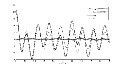
Figure 2: Profiles of the kernels function for subspace-I: The first two entries $\theta_{11}(t)$ and $\theta_{12}(t)$ of the exact kernel function (lines without markers) produced by brutal-force computation according to (32) and approximated kernel (48) using the Krylov space method (lines with markers) with order 4. These two entries are corresponding to the correlations of the noises in the first two translational modes of the first rigid block.

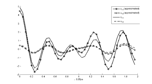
Figure 3: Profiles of the kernels function for subspace-II: The first two entries of the exact kernel function (lines without markers) produced by directly computation according to (32) and the approximated kernel (48) using the Krylov space method and subspace-II (lines with markers). These two entries are corresponding to the correlations of the noises in the first two translational modes of the first rigid block. The order of the Krylov space is 4.

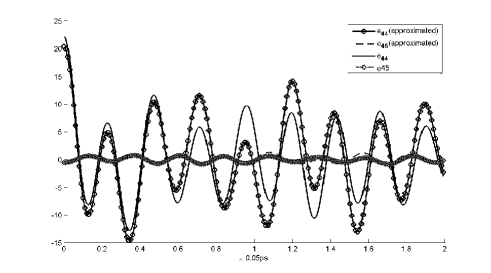
Figure 4: Profiles of the kernels function for subspace-I: The first two entries of the exact kernel function (lines without markers) produced by brutal-force computation and the approximated kernel (48) using Krylov space method (lines with markers) with order 4. These two entries are corresponding to the correlations of the noises in the first two rotational modes of the first rigid block.

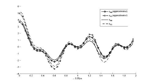
Figure 5: Profiles of the kernels function for subspace-II: Two entries of the kernel function (lines without markers) produced by directly computation and the the approximated kernel using Krylov space method (lines with markers). These two entries are corresponding to the correlations of the noises in the first two rotational modes of the first rigid block. The order of the Krylov space is 4.

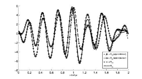
Figure 6: Profiles of the kernels function for subspace-III: The first two entries of the exact kernel function produced by directly computation (lines without markers) and the approximated kernel using the Krylov space method (lines with markers) using subspace-III. The order of the Krylov space is 4.

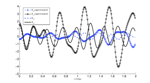
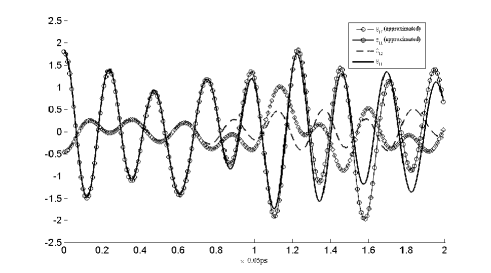
Figure 7: Profiles of the first two entries of the exact kernel function produced by directly computation (lines without markers) and the approximated kernel using the Krylov method (lines with markers) for subspace-I. Top: Krylov space with order 2; Bottom: Krylov space with order 6.

Fig. 3 also indicates that the memory functions for the residue-based subspaces look smoother. This is because the residue-based subspaces admit more low frequency modes than those of rigid bodies from the partitions of PROFLEX.

Next, we consider the same type of partitions (subspace -II based on residues), but with different block sizes. In particular, we first start with a fine partition, in which each residue is a block. We then form a coarser partition, where there are 3 residues in each block (It is clear that this partition is not based on the flexibility of the molecule). One observes from Fig. 8 that the memory functions become smaller for the coarser partition.

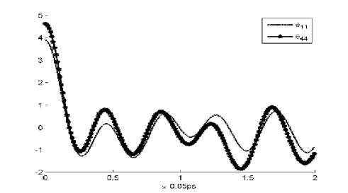
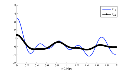
Figure 8: Profiles of the two entries of the exact kernel function produced by directly computation. The coarse grained subspace are spanned by the RTB basis corresponding to the following partition. Top: 1 residue as a rigid block; Bottom: 3 residues in each block.

To further confirm this observation, we divide the entire system equally into 22 blocks with 9 residues in each block. We also form a 6-block partition, each of which contains 33 residues. The results, shown in Fig. 9, exhibit the same trend: as we coarse-grain more and more, the memory functions become smaller and smaller.

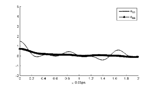
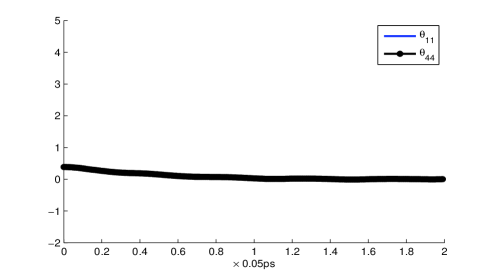
Figure 9: Profiles of the first two entries of the exact kernel function produced by directly computation. The coarse grained subspace are spanned by the RTB basis corresponding to the following partition. Top 33: residues in each block; Bottom: 9 residues in one rigid block.

V Discussion

In this paper, we have presented a methodology to compute memory functions which are important parameters in the generalized Langevin model. Computing such memory functions directly from molecular dynamics simulations would require extensive effort. In contrast, the method proposed here relies on a technique in numerical linear algebra, and it can be implemented without performing molecular simulations.

We have also demonstrated that under the current framework, the random noise term in the generalized Langevin equation can be consistently approximated. To our knowledge, none of the existing methods offers such advantage. Together with the average force $F(\bm{q})$, the generalized Langevin equation can be solved to describe the collective motion of the system. This is work in progress.

VI Acknowledgement

The work has been partially supported by NSF grants DMS–1109107, DMS-1216938, and DMS-1159937. This work was initialized during Chen’s visitation to the Department of Mathematics, at the Pennsylvania State University. He would like to thank the hospitality of the department. M.X. Chen was supported by the China NSF (NSFC11301368) and the NSF of Jiangsu Province (BK20130278).

References

- Schlick (2002) T. Schlick, Molecular Modeling and Simulation: An Interdisciplinary Guide (Springer-Verlag, 2002).
- Leach (2001) A. Leach, Molecular Modelling: Principles and Applications (Prentice Hall, 2001).
- Baaden and Marrink (2013) M. Baaden and S. J. Marrink, “Coarse-grain modelling of protein-protein interactions,” Curr. Opin. Struct. Biol. In press. (2013).
- Gohlke and Thorpe (2006) H. Gohlke and M. Thorpe, “A natural coarse graining for simulating large biomolecular motion,” Biophys. J. 91, 2115–2120 (2006).
- Noid (2013) W. G. Noid, “Perspective: coarse-grained models for biomolecular systems,” J. Chem. Phys. 139, 090901 (2013).
- Noid et al. (2008) W. G. Noid, J.-W. Chu, G. S. Ayton, V. Krishna, S. Izvekov, G. A. Voth, A. Das, and H. C. Andersen, “The multiscale coarse-graining method. I. a rigorous bridge between atomistic and coarse-grained models,” J. Chem. Phys. 128, 244114 (2008).
- Praprotnik, Site, and Kremer (2008) M. Praprotnik, L. D. Site, and K. Kremer, “Multiscale simulation of soft matter: from scale bridging to adaptive resolution,” Annu. Rev. Phys. Chem. 59, 545–571 (2008).
- Riniker, Allison, and van Gunsteren (2012) S. Riniker, J. R. Allison, and W. F. van Gunsteren, “On developing coarse-grained models for biomolecular simulation: a review,” Phys. Chem. Ch. Ph. 14, 12423 (2012).
- Rudzinski and Noid (2012) J. F. Rudzinski and W. G. Noid, “The role of many-body correlations in determining potentials for coarse-grained models of equilibrium structure,” J. Phys. Chem. B 116, 8621–8635 (2012).
- Chorin, Kast, and Kupferman (1998) A. J. Chorin, A. Kast, and R. Kupferman, “Optimal prediction of underresolved dynamics,” Proc. Nat. Acad. Sci. USA 96, 4094 – 4098 (1998).
- Chorin, Hald, and Kupferman (2002) A. J. Chorin, O. H. Hald, and R. Kupferman, “Optimal prediction with memory,” Phys. D 166, 239–257 (2002).
- Mori (1965) H. Mori, “Transport, collective motion, and Brownian motion,” Prog. Theor. Phys. 33, 423 – 450 (1965).
- Zwanzig (1973) R. Zwanzig, “Nonlinear generalized Langevin equations,” J. Stat. Phys. 9, 215 – 220 (1973).
- Berkowitz, Morgan, and McCammon (1983) M. Berkowitz, J. Morgan, and J. A. McCammon, “Generalized Langevin dynamics simulations with arbitrary time-dependent memory kernels,” J. Chem. Phys. 78, 3256 (1983).
- Bu and Straub (2003) L. Bu and J. E. Straub, “Vibrational frequency shifts and relaxation rates for a selected vibrational mode in cytochrome c,” Biophys. J. 85, 1429–1439 (2003).
- Izvekov and Voth (2006) S. Izvekov and G. A. Voth, “Modeling real dynamics in the coarse-grained representation of condensed phase systems,” J. Chem. Phys. 125, 151101–151104 (2006).
- Kamberaj (2011) H. Kamberaj, “A theoretical model for the collective motion of proteins by means of principal component analysis,” Cent. Eur. J. Phys. 9, 96–109 (2011).
- Lange and Grubmüller (2006) O. F. Lange and H. Grubmüller, “Collective Langevin dynamics of conformational motions in proteins,” J. Chem. Phys. 124, 214903 (2006).
- Oliva et al. (2000) B. Oliva, X. Daura, E. Querol, F. X. Avilés, and O. Tapia, “A generalized langevin dynamics approach to model solvent dynamics effects on proteins via a solvent-accessible surface. the carboxypeptidase a inhibitor protein as a model,” Theor. Chem. Acc. 105, 101–109 (2000).
- Sagnella, Straub, and Thirumalai (2000) D. E. Sagnella, J. E. Straub, and D. Thirumalai, “Time scales and pathways for kinetic energy relaxation in solvated proteins: Application to carbonmonoxy myoglobin,” J. Chem. Phys. 113, 7702 (2000).
- Stepanova (2007) M. Stepanova, “Dynamics of essential collective motions in proteins: Theory,” Phys. Rev. E 76, 051918 (2007).
- Zwanzig (1961) R. Zwanzig, “Statistical mechanics of irreversiblity,” Lectures in Theoretical Physics 3, 106–141 (1961).
- Li (2010) X. Li, “A coarse-grained molecular dynamics model for crystalline solids,” Int. J. Numer. Meth. Engng. 83, 986–997 (2010).
- Chorin and Stinis (2005) A. J. Chorin and P. Stinis, “Problem reduction, renormalization, and memory,” Comm. Appl. Math. Comp. Sc. 1, 1–27 (2005).
- Kubo (1966) R. Kubo, “The fluctuation-dissipation theorem,” Rep. Prog. Phys. 29(1), 255 – 284 (1966).
- Hijón, Serrano, and Español (2006) C. Hijón, M. Serrano, and P. Español, “Markovian approximation in a coarse-grained description of atomic systems,” J. Chem. Phys. 125, 204101 (2006).
- Kauzlarić et al. (2011) D. Kauzlarić, J. T. Meier, P. Español, S. Succi, A. Greiner, and J. G. Korvink, “Bottom-up coarse-graining of a simple graphene model: The blob picture,” J. Chem. Phys. 134, 064106–064106 (2011).
- Kauzlarić et al. (2012) D. Kauzlarić, P. Español, A. Greiner, and S. Succi, “Markovian dissipative coarse grained molecular dynamics for a simple 2d graphene model,” The Journal of chemical physics 137, 234103 (2012).
- Berkowitz et al. (1981) M. Berkowitz, J. D. Morgan, D. J. Kouri, and J. A. McCammon, “Memory kernels from molecular dynamics,” J. Chem. Phys. 75, 2462–2463 (1981).
- Balescu (1976) R. Balescu, Equilibrium and Nonequilibrium Statistical Mechanics (John Wiley & Sons, 1976).
- Evans and Morriss (2008) D. J. Evans and G. P. Morriss, Statistical Mechanics of Nonequilibrium Liquids (ACADEMIC PRESS, 2008).
- Zwanzig (2001) R. Zwanzig, Nonequilibrium Statistical Mechanics (Oxford University Press, 2001).
- Arnol’d (1989) V. I. Arnol’d, Mathematical methods of classical mechanics, Vol. 60 (Springer, 1989).
- Li (2014) X. Li, “Coarse-graining molecular dynamics models using an extended Galerkin projection,” Int. J. Numer. Meth. Engng. to appear (2014).
- Note (1) This linearization is again the reference position, in which case the matrix is the hessian of the potential energy. This seems to be the only way to obtain a linear convolutional form of the memory function.
- Yanai, Takeuchi, and Takane (2011) H. Yanai, K. Takeuchi, and Y. Takane, Projection Matrices (Springer, 2011).
- Note (2) Otherwise a nonlinear convolution term appear. Such an approximation is appropriate when the system is around the reference position. But the error would be large during structural change, in which case it would be necessary to keep this term.
- Doob (1944) J. L. Doob, “The elementary gaussian processes,” Ann. Math. Stat. 15, 229–282 (1944).
- Saad (1992) Y. Saad, “Analysis of some Krylov subspace approximations to the matrix exponential operator,” SIAM J. Numer. Anal. 29, 209–228 (1992).
- Diele, Moret, and Ragni (2009) F. Diele, I. Moret, and S. Ragni, “Error estimates for polynomial Krylov approximations to matrix functions,” SIAM J. Matrix Anal. Appl. 30, 1546–1565 (2009).
- Saad (2003) Y. Saad, Iterative Methods for Sparse Linear Systems, second edition ed. (SIAM, 2003).
- Li and Cui (2002) G. Li and Q. Cui, “A coarse-grained normal mode approach for macromolecules: an efficient implementation and application to -atpase,” Biophys. J. 83, 2457–2474 (2002).
- F. Tama and Sanejouand (2000) O. M. F. Tama, F. X. Gadea and Y. Sanejouand, “Building-block approach for determining low-frequency normal modes of macromolecules,” Proteins 41, 1–7 (2000).
- Demerdash and Mitchell (2012) O. N. A. Demerdash and J. C. Mitchell, “Density-cluster nma: A new protein decomposition technique for coarse-grained normal mode analysis,” Proteins 80, 1766–1779 (2012).
- Wilson, Decius, and Cross (1980) E. B. Wilson, J. C. Decius, and P. C. Cross, Molecular Vibrations: The Theory of Infrared and Raman Vibrational Spectra (Dover, 1980).
- Ye (1996) Q. Ye, “An adaptive block Lanczos algorithm,” Numer. Algorithms 12, 97–110 (1996).
- Jacobs et al. (2001) D. J. Jacobs, A. J. Rader, L. A. Kuhn, and M. F. Thorpe, “Protein flexibility predictions using graph theory,” Proteins 44, 150–165 (2001).
- Tatsuoka (1988) M. M. Tatsuoka, Multivariate Analysis (Macmillian, New York, 1988).