Metric Space Formulation of Quantum Mechanical Conservation Laws

Abstract

We show that conservation laws in quantum mechanics naturally lead to metric spaces for the set of related physical quantities. All such metric spaces have an “onion-shell” geometry. We demonstrate the power of this approach by considering many-body systems immersed in a magnetic field, with a finite ground state current. In the associated metric spaces we find regions of allowed and forbidden distances, a “band structure” in metric space directly arising from the conservation of the $z$ component of the angular momentum.

I Introduction

Conservation laws are a central tenet of our understanding of the physical world. Their tight relationship to natural symmetries was demonstrated by Noether in 1918 Noether (1918) and has since been a fundamental tool for developing theoretical physics. In this paper we demonstrate how these laws induce appropriate “natural” metrics on the related physical quantities. Conservation laws are central to the behavior of physical systems and we show how this relevant physics is translated into the metric analysis. We argue that this alternative picture provides a new powerful tool to study certain properties of many-body systems, which are often complex and hardly tractable when considered within the usual coordinate space-based analysis, while may become much simpler when analyzed within metric spaces. We exemplify this concept by considering functional relationships fundamental to current density functional theory (CDFT) Vignale and Rasolt (1987, 1988).

We will first introduce a way to derive appropriate “natural” metrics from a system’s conservation laws. Second, as an example application of the approach, we will explicitly consider an important class of systems – systems with applied external magnetic fields. In contrast with those to which standard density functional theory (DFT) Dreizler and Gross (1990) can be applied, systems subject to external magnetic fields are not simply characterized by their particle densities as even their ground states may display a finite current Vignale and Rasolt (1987, 1988). These systems are of great importance, e.g., due to the emerging quantum technologies of spintronics and quantum information where, for example, few electrons in nano- or microstructures immersed in magnetic fields are proposed as hardware units Takahashi et al. (2010); Dias da Silva et al. (2009); Brandner et al. (2013); Amaha et al. (2013); Castellanos-Beltran et al. (2013).

To analyze systems immersed in a magnetic field, we will introduce a metric associated with the paramagnetic current density, which can be associated with the angular momentum components. We will show that, at least for systems which preserve the $z$ component of the angular momentum, the paramagnetic current density metric space displays an “onion-shell” geometry, directly descending from the related conservation law. In recent work D’Amico et al. (2011a); Artacho (2011); D’Amico et al. (2011b) appropriate metrics for characterizing wavefunctions and particle densities within quantum mechanics were introduced. It was shown that wavefunctions and their particle densities both form metric spaces with an “onion-shell” structure D’Amico et al. (2011a). We will show that, within the same general procedure used for the paramagnetic current, these metrics descend from the respective conservation laws. We will then focus on ground states and characterize them not only through the mapping between wavefunctions and particle densities, but importantly through mappings involving the paramagnetic current density. In fact, for systems with an applied magnetic field, ground state wavefunctions are characterized uniquely only by knowledge of both particle and paramagnetic current densities (and vice versa), as demonstrated within CDFT Vignale and Rasolt (1987, 1988).

The rest of this paper is organized as follows: In Sec. II we introduce our general approach to derive metric spaces from conservation laws. We demonstrate the application of this approach to wavefunctions, particle densities, and paramagnetic current densities in Sec. III. We consider systems subject to magnetic fields in Sec. IV. Here we use the metrics derived from our approach to study the fundamental theorem of CDFT. We present our conclusions in Sec. V.

II Derivation of Metric Spaces from Conservation Laws

A metric or distance function $D$ over a set $X$ satisfies the following axioms for all $x,y,z\in X$ Megginson (1998); Sutherland (2009):

$$D(x,y) \geqslant 0\ \text{and}\ D(x,y)=0\iff x=y,$$ (1)

$$D(x,y) =D(y,x),$$ (2)

$$D(x,y) \leqslant D(x,z)+D(z,y),$$ (3)

with (3) known as the triangle inequality. The set $X$ with the metric $D$ forms the metric space $(X,D)$. It can be seen from the axioms (1) - (3) that many metrics could be devised for the same set, some trivial. Here we introduce “natural” metrics associated to conservation laws: this will avoid arbitrariness and in turn will ensure that the proposed metrics stem from core characteristics of the systems analyzed and contain the related physics.

In quantum mechanics, many conservation laws take the form

$$\int\left|f(x)\right|^{p}dx=c$$ (4)

for $0<c<\infty$. For each value of $1\leqslant p<\infty$, the entire set of functions that satisfy (4) belong to the $L^{p}$ vector space, where the standard norm is the $p$ norm Megginson (1998)

$$\left|\left|f(x)\right|\right|_{p}=\left[\int\left|f(x)\right|^{p}dx\right]^{\frac{1}{p}}.$$ (5)

From any norm a metric can be introduced in a standard way as $D(x,y)=\left|\left|x-y\right|\right|$ so that with $p$ norms we get

$$D_{f}(f_{1},f_{2}):=\left|\left|f_{1}-f_{2}\right|\right|_{p}.$$ (6)

However before assuming this metric for the physical functions related to the conservation laws, an important consideration must be made: Eq. (6) has been derived assuming the ensemble $\{f\}$ to be a vector space; this is in fact necessary to introduce a norm. If we want to retain the metric (6), but restrict it to the ensemble of physical functions satisfying (4), which does not necessarily form a vector space, we must show that (6) is a metric for this restricted function set. This can be done using the general theory of metric spaces: given a metric space $(X,D)$ and $S$ a non empty subset of $X$, $(S,D)$ is itself a metric space with the metric $D$ inherited from $(X,D)$. The metric axioms (1) - (3) automatically hold for $(S,D)$ because they hold for $(X,D)$ Megginson (1998); Sutherland (2009). Hence, we have a metric for the functions of interest, as their sets are non empty subsets of the respective $L^{p}$ sets.

The metric (6) is then the one that directly descends from the conservation law (4). Conversely any conservation law which can be recast as (4) (for example conservation of quantum numbers) can be interpreted as inducing a metric on the appropriate, physically relevant, subset of $L^{p}$ functions. This provides a general procedure to derive “natural” metrics from physical conservation laws.

III Applications of the Metric Space Approach

We now consider specific quantum mechanical functions and conservation laws. Following Ref. D’Amico et al. (2011a) we use a convention where wavefunctions are normalized to the particle number $N$ . Then the particle density of an $N$-particle system and its paramagnetic current density are defined as

$$\rho(\mathbf{r}) =\int\left|\psi\left(\mathbf{r},\mathbf{r}_{2},\ldots,\mathbf{r}_{N}\right)\right|^{2}d\mathbf{r}_{2}\ldots d\mathbf{r}_{N},$$ (7)

$$\mathbf{j}_{p}(\mathbf{r}) =-\frac{i}{2}\int\left(\psi^{\ast}\nabla\psi-\psi\nabla\psi^{\ast}\right)d\mathbf{r}_{2}\ldots d\mathbf{r}_{N}.$$ (8)

First of all we note that $\psi\left(\mathbf{r}_{1},\mathbf{r}_{2},\ldots,\mathbf{r}_{N}\right)$ and $\rho(\mathbf{r})$ are subject to the following conservation laws (wavefunction norm and particle conservation):

$$\int\left|\frac{\psi\left(\mathbf{r}_{1},\mathbf{r}_{2},\ldots,\mathbf{r}_{N}\right)}{\sqrt{N}}\right|^{2}d\mathbf{r}_{1}\ldots d\mathbf{r}_{N}=1,$$ (9)

$$\int\rho(\mathbf{r})d\mathbf{r}=N.$$ (10)

Similarly the paramagnetic current density $\mathbf{j}_{p}(\mathbf{r})$ obeys

$$\int\left[\mathbf{r}\times\mathbf{j}_{p}(\mathbf{r})\right]_{z}d\mathbf{r}=\langle\psi|\hat{L}_{z}|\psi\rangle.$$ (11)

For eigenstates of systems for which the $z$ component of the angular momentum is preserved we then have $\langle\hat{L}_{z}\rangle=m$, with $m$ an integer, and (11) can be recast as

$$\int\left|\left[\mathbf{r}\times\mathbf{j}_{p}(\mathbf{r})\right]_{z}\right|d\mathbf{r}=\left|m\right|.$$ (12)

For wavefunctions and particle densities our procedure leads to the metrics introduced in Ref. D’Amico et al. (2011a) ($N$ fixed) Artacho (2011); D’Amico et al. (2011b)

$$D_{\psi}(\psi_{1},\psi_{2})= \left[\int\left(\left|\psi_{1}\right|^{2}+\left|\psi_{2}\right|^{2}\right)d\mathbf{r}_{1}\ldots d\mathbf{r}_{N}\right.$$

$$-\left.2\left|\int\psi_{1}^{*}\psi_{2}d\mathbf{r}_{1}\ldots d\mathbf{r}_{N}\right|\right]^{\frac{1}{2}},$$ (13)

$$D_{\rho}(\rho_{1},\rho_{2})= \int\left|\rho_{1}(\mathbf{r})-\rho_{2}(\mathbf{r})\right|d\mathbf{r};$$ (14)

for the paramagnetic current density, our procedure introduces the following metric:

$$D_{\mathbf{j}_{p_{\perp}}}(\mathbf{j}_{p,1},\mathbf{j}_{p,2})=\int\left|\left\{\mathbf{r}\times\left[\mathbf{j}_{p,1}(\mathbf{r})-\mathbf{j}_{p,2}(\mathbf{r})\right]\right\}_{z}\right|d\mathbf{r}.$$ (15)

We note that $D_{\mathbf{j}_{p_{\perp}}}$ will be a distance between equivalence classes of paramagnetic currents, each class characterized by current densities having the same transverse component $\mathbf{j}_{p_{\perp}}\equiv(j_{p,x},j_{p,y})$. $D_{\mathbf{j}_{p_{\perp}}}$ is gauge invariant provided that $\mathbf{j}_{p,1}$ and $\mathbf{j}_{p,2}$ are within the same gauge and $[\hat{L_{z}},\hat{H}]=0$.

Next we show that conservation laws naturally build within the related metric spaces a hierarchy of concentric spheres, or “onion-shell” geometry. If we set as the center of each sphere the zero function $f^{(0)}(x)\equiv 0$, and consider the distance between it and any other element in the metric space, we recover the $p$-norm expressions (5) directly descending from the related conservation laws. This procedure induces in the related metric spaces a structure of concentric spheres with radii, in the cases considered here, of natural numbers to the power of $1/p$: all functions corresponding to the same value of a certain conserved quantity will lay on the surface of the same sphere. Specifically, for systems of $N$ particles, wavefunctions lie on spheres of radius $\sqrt{N}$, and particle densities on spheres of radius $N$; for the metric space of paramagnetic current densities, all paramagnetic current densities with a $z$ component of the angular momentum equal to $\pm m$ lie on spheres of radius $\left|m\right|$.

The first axiom of a metric (1) guarantees that the minimum value for all distances is $0$, and that this value is attained for two identical states. The onion-shell geometry guarantees that, for functions on the surface of the same sphere, i.e., which satisfy a certain conservation law with the same value, there is also an upper limit for their distance associated with the diameter of the sphere. From (15) we see that for paramagnetic current densities this upper limit is achieved in the limit of currents which do not spatially overlap. This is also the case for particle densities, as seen in (14).

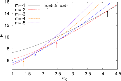
Figure 1: (Color online) For the ISI system energy is plotted against the confinement frequency for several values of the angular momentum quantum number $m$ (as labeled), and with constant cyclotron frequency and interaction strength. Arrows indicate where the value of $m$ for the ground state changes.

Interestingly, and in contrast to wavefunctions and particle densities D’Amico et al. (2011a), even when considering systems with the same number of particles it may be necessary to consider paramagnetic current densities with different values of $m$; in terms of their metric space geometry, current densities that have different values of $\left|m\right|$ lie on different spheres. Therefore, the maximum value for the distance between paramagnetic current densities of a system of $N$ particles is related to the upper limit of the number of spheres in the onion-shell geometry. Using the triangle inequality we have in fact

$$D_{\mathbf{j}_{p_{\perp}}}(\mathbf{j}_{p,m_{1}},\mathbf{j}_{p,m_{2}}) \leqslant D_{\mathbf{j}_{p_{\perp}}}(\mathbf{j}_{p,m_{1}},\mathbf{j}^{(0)}_{p})+D_{\mathbf{j}_{p_{\perp}}}(\mathbf{j}^{(0)}_{p},\mathbf{j}_{p,m_{2}})$$

$$=\left|m_{1}\right|+\left|m_{2}\right|\leqslant l_{1}+l_{2},$$ (16)

where $l_{i}$ is the quantum number related to the total angular momentum of system $i$.

IV Study of Model Systems

We now concentrate on the sets of ground state wavefunctions, related particle densities, and related paramagnetic current densities. Since ground states are non empty subsets of all states, ground-state-related functions form metric spaces with the metrics (13), (14), and (15). The importance of characterizing ground states and their properties has been highlighted by the huge success of DFT (in all its flavors) as a method to predict devices’ and material properties Dreizler and Gross (1990); Ullrich and Yang (2013). Standard DFT is built on the Hohenberg-Kohn (DFT-HK) theorem Hohenberg and Kohn (1964), which demonstrates a one-to-one mapping between ground state wavefunctions and their particle densities. This theorem is highly complex and nonlinear in coordinate space. However, Ref. D’Amico et al. (2011a) showed that the DFT-HK theorem is a mapping between metric spaces, and may be very simple when described in these terms, becoming monotonic and almost linear for a wide range of parameters and for the systems there analyzed. CDFT is a formulation of DFT for systems in the presence of an external magnetic field. In CDFT Vignale and Rasolt (1987, 1988) the original HK mapping is extended (CDFT-HK theorem) to demonstrate that $\psi$ is uniquely determined only by knowledge of both $\rho(\mathbf{r})$ and $\mathbf{j}_{p}(\mathbf{r})$ (and vice versa). This is the theorem we will consider in this section.

To further our analysis, we now explicitly examine two model systems with applied magnetic fields. They both consist of two electrons parabolically confined that interact via different potentials, Coulomb (magnetic Hooke’s atom) Taut et al. (2009) and inverse square interaction (ISI) Quiroga et al. (1993), respectively. Both systems may be used to model electrons confined in quantum dots. The Hamiltonians for the magnetic Hooke’s atom and the ISI system are

$$\hat{H}_{HA} =\sum_{i=1}^{2}\left\{\frac{1}{2}\left[\hat{\mathbf{p}}_{i}+\mathbf{A}\left(\mathbf{r}_{i}\right)\right]^{2}+\frac{1}{2}\omega_{0}^{2}r_{i}^{2}\right\}+\frac{1}{\left|\mathbf{r}_{2}-\mathbf{r}_{1}\right|},$$ (17)

$$\hat{H}_{ISI} =\sum_{i=1}^{2}\left\{\frac{1}{2}\left[\hat{\mathbf{p}}_{i}+\mathbf{A}\left(\mathbf{r}_{i}\right)\right]^{2}+\frac{1}{2}\omega_{0}^{2}r_{i}^{2}\right\}+\frac{\alpha}{\left(\mathbf{r}_{1}-\mathbf{r}_{2}\right)^{2}},$$ (18)

(atomic units, $\hbar=m_{e}=e=1$). Here $\alpha$ is a positive constant, $\mathbf{A}=\frac{1}{2}\mathbf{B}\times\mathbf{r}$ (symmetric gauge), and $\mathbf{B}=\omega_{c}c\mathbf{\hat{z}}$ is a homogeneous, time-independent external magnetic field. For these systems $\langle\hat{L}_{z}\rangle$ is a conserved quantity. Following Refs. Vignale and Rasolt (1987); Taut et al. (2009) we disregard spin to concentrate on the features of the orbital currents. For Hooke’s atom, we obtain highly precise numerical solutions following the method in Ref. Coe et al. (2008). The ISI system is solved exactly Quiroga et al. (1993).

Figure 2: Results for ground states. Top: Hooke’s atom (reference state ${\omega}_{0}=0.5,{\omega}_{c}=5,m_{ref}=-5$). Bottom: ISI system (reference state ${\omega}_{0}=0.62,{\omega}_{c}=5.5,{\alpha}=5,m_{ref}=-10$). Panels (a) and (b): $D_{\rho}$ vs $D_{\psi}$; (c) and (d): rescaled $D_{\mathbf{j}_{p_{\perp}}}$ vs $D_{\psi}$; (e) and (f): rescaled $D_{\mathbf{j}_{p_{\perp}}}$ vs $D_{\rho}$. Frequencies smaller than the reference are labeled with circles, larger with triangles.

To produce families of ground states, for each system we systematically vary the value of $\omega_{0}$ (while keeping all other parameters constant), and for each value we calculate the ground state wavefunction, particle density, and paramagnetic current density. A reference state is determined by choosing a specific $\omega_{0}$ value, and the appropriate metric is then used to calculate the distances between it and each member of the family. To ensure that we select ground states, varying $\omega_{0}$ may require varying the quantum number $m$ Taut et al. (2009); Quiroga et al. (1993). This is shown for the ISI system in Fig. 1. Here, as $\omega_{0}$ increases, we must decrease the value of $\left|m\right|$ in order to remain in the ground state. As a result of this property, within each family of ground states, paramagnetic current densities will “jump” from one sphere of the onion-shell geometry to another [see Fig. 3(a), where the reference state is the ‘north pole’ of its sphere]. To obtain ground states with nonzero paramagnetic currents, we must use $\omega_{0}$ values corresponding to $m<0$ Taut et al. (2009); Quiroga et al. (1993).

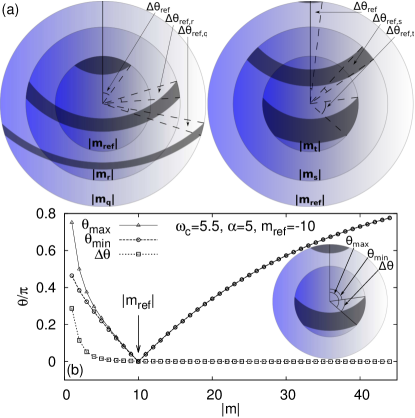
Figure 3: (Color online) (a) Sketch of the onion-shell geometry of the metric space for paramagnetic current densities, where $\left|m_{q}\right|>\left|m_{r}\right|>\left|m_{ref}\right|$ (left) and $\left|m_{ref}\right|>\left|m_{s}\right|>\left|m_{t}\right|$ (right). The reference state is at the north pole on the reference sphere. The dark gray areas denote the regions where ground state currents are located (‘bands’), with dashed lines indicating their widths. (b) Results of the angular displacement of ground state currents for the ISI system. Lines are a guide to the eye. Inset: Definition of relevant angles.

In Fig. 2, we plot each pair of distances for the two systems. The reference states have been chosen so that most of the available distance range can be explored both for the case of increasing and for the case of decreasing values of $\omega_{0}$. When considering the relationship between ground state wavefunctions and related particle densities, Figs. 2(a) and 2(b), our results confirm the findings in Ref. D’Amico et al. (2011a): a monotonic mapping, linear for low to intermediate distances, and where vicinities are mapped onto vicinities; also curves for increasing and decreasing $\omega_{0}$ collapse onto each other. However closer inspection reveals a fundamental difference with Ref. D’Amico et al. (2011a), the presence of a “band structure.” By this we mean regions of allowed (“bands”) and forbidden (“gaps”) distances, whose widths depend, for the systems considered here, on the value of $\left|m\right|$. This structure is due to the changes in the value of the quantum number $m$, which result in a substantial modification of the ground state wavefunction (and therefore density) and a subsequent large increase in the related distances.

When we focus on the plots of paramagnetic current densities’ against wavefunctions’ distances, Figs. 2(c) and 2(d), we find that the “band structure” dominates the behavior. Here the change in $\left|m\right|$ has an even stronger effect, in that $dD_{\mathbf{j}_{p_{\perp}}}/dD_{\psi}$ is noticeably discontinuous when moving from one sphere to the next in $\mathbf{j}_{p}$ metric space. This discontinuity is more pronounced for the path $\left|m\right|<\left|m_{ref}\right|$ than for the path $\left|m\right|>\left|m_{ref}\right|$. Similarly to Figs. 2(a) and 2(b), the mapping of $D_{\psi}$ onto $D_{\mathbf{j}_{p_{\perp}}}$ maps vicinities onto vicinities and remains monotonic, but for small and intermediate distances it is only piecewise linear. In contrast with $D_{\rho}$ vs $D_{\psi}$, curves corresponding to increasing and decreasing $\omega_{0}$ do not collapse onto each other.

Figures 2(e) and 2(f) show the mapping between particle and paramagnetic current density distances: this has characteristics similar to the one between $D_{\psi}$ and $D_{\mathbf{j}_{p_{\perp}}}$, but remains piecewise linear even at large distances.

We will now concentrate on the $\mathbf{j}_{p}$ metric space to characterize the “band structure” observed in Fig. 2. Within the metric space geometry, we consider the polar angle $\theta$ between the reference $\mathbf{j}_{p,ref}$ and the paramagnetic current density $\mathbf{j}_{p}$ of angular momentum $\left|m\right|$. Using the law of cosines, $\theta$ is given by

$$\cos{\theta}=\frac{m_{ref}^{2}+m^{2}-D_{\mathbf{j}_{p_{\perp}}}^{2}(\mathbf{j}_{p,ref},\mathbf{j}_{p})}{2\left|m_{ref}\right|\left|m\right|}.$$ (19)

We define the polar angles corresponding to the two extremes of a given band as $\theta_{min}$ and $\theta_{max}$ (inset of Fig. 3). The width of each band is then ${\Delta}{\theta}={\theta}_{max}-{\theta}_{min}$, and its position defined by $\theta_{min}$. Now we can calculate the bands’ widths and positions by sweeping, for each $\left|m\right|$, the values of $\omega_{0}$ corresponding to ground states (Fig. 3).

For both systems under study, we find that as $\left|m\right|$ increases from $\left|m_{ref}\right|$, both ${\theta}_{max}$ and ${\theta}_{min}$ increase. This has the effect of the bands moving from the north pole to the south pole as we move away from the reference. Additionally, we find that the bandwidth ${\Delta}{\theta}$ decreases as $\left|m\right|$ increases [sketched in Fig. 3(a), left]. As $\left|m\right|$ decreases from $\left|m_{ref}\right|$, we again find that both ${\theta}_{max}$ and ${\theta}_{min}$ increase, with the bands moving from the north pole to the south pole. However, this time, as $\left|m\right|$ decreases, ${\Delta}{\theta}$ increases, meaning that the bands get wider as we move away from the reference [sketched in Fig. 3(a), right].

Quantitative results for the ISI system are shown in Fig. 3(b). We obtain similar results for Hooke’s atom (not shown). The band on the surface of each sphere indicates where all ground state paramagnetic current densities lie within that sphere. In contrast with particle densities or wavefunctions, we find that, at least for the systems at hand, ground state currents populate a well-defined, limited region of each sphere, whose size and position display monotonic behavior with respect to the quantum number $m$. This regular behavior is not at all expected, as the CDFT-HK theorem does not guarantee monotonicity in metric space, and not even that the mapping of $D_{\psi}$ to $D_{\mathbf{j}_{p_{\perp}}}$ is single valued. In the CDFT-HK theorem ground state wavefunctions are uniquely determined only by particle and paramagnetic current densities together. In this sense we can look at the panels in Fig. 2 as projections on the axis planes of a 3-dimensional $D_{\psi}D_{\rho}D_{\mathbf{j}_{p_{\perp}}}$ relation. The complexity of the mapping due to the application of a magnetic field – the changes in quantum number $m$ – is fully captured by $D_{\mathbf{j}_{p_{\perp}}}$ only, as this is related to the relevant conservation law. However the mapping from $D_{\rho}$ to $D_{\psi}$ inherits the “band structure,” showing that the two mappings $D_{\mathbf{j}_{p_{\perp}}}$ to $D_{\psi}$ and $D_{\rho}$ to $D_{\psi}$ are not independent.

V Conclusion

In conclusion we showed that conservation laws induce related metric spaces with an “onion-shell” geometry and that they may induce a “band structure” in ground state metric spaces, a signature of the enhanced constraints due to the system conservation laws on the relation between wavefunctions and the relevant physical quantities.

The method proposed may help with understanding extended HK theorems, such as, in the case at hand, the CDFT-HK theorem. In this respect we find that in metric spaces and for the systems considered, the relevant mappings display distinctive signatures, including (piecewise) linearity at short and medium distances, the mapping between ground state $\psi$ and $\mathbf{j}_{p}$ resembling the one between $\rho$ and $\mathbf{j}_{p}$, and the mapping between ground state $\psi$ and $\mathbf{j}_{p}$ showing different trajectories for increasing or decreasing Hamiltonian parameters, in contrast with the mapping between $\psi$ and $\rho$. Features like this could be used to build or test (single-particle) approximate solutions to many-body problems, e.g., within DFT schemes.

Our results show that using conservation laws to derive metrics makes these metrics a powerful tool to study many-body systems governed by integral conservation laws.