Abstract

We present a solution of the quantum mechanics problem of the allowable energy levels of a bound particle in a one-dimensional finite square well. The method is a geometric-analytic technique utilizing the conformal mapping $w\to z=we^{w}$ between two complex domains. The solution of the finite square well problem can be seen to be described by the images of simple geometric shapes, lines and circles, under this map and its inverse image. The technique can also be described using the Lambert W function. One can work in either of the complex domains, thereby obtaining additional insight into the finite square well problem and its bound energy states. There are many opportunities to follow up, and we present the method in a pedagogical manner to stimulate further research in this and related avenues.

1 Introduction

Quantum well models are important for the design of semiconductor devices, such as the quantum well infrared photodetector (QWIP) which is used for infrared imaging applications; see Schneider and Liu [1] for an overview. The QWIP relies upon a quantum well which has been sized so that the energy of an electron in the first excited state is quite near the threshold of confinement in the well. The QWIP is therefore very sensitive to the arrival of a single photon. There are many other uses of quantum well models in nanostructures; the textbook by Harrison [2] is a good survey of the field.

The one-dimensional quantum finite square well (FSW) model is a familiar topic in most introductory quantum mechanics books; see for instance Bransden and Joachain [3], section 4.6. After deriving a pair of equations to describe the bound energy levels within the well, the solution is carried out by graphical or computational methods. It is sometimes said that the FSW problem does not have an exact solution, but there are in fact exact solutions as presented in the papers of Burniston and Siewert [4, 5, 6] and others [7, 8, 9, 10, 11, 12]. Those exact methods generally rely upon contour integration in the complex plane.

We have found a simple geometric method which can be used to describe the solutions of the one-dimensional finite square well problem. Our approach is analytic, using complex variables, but does not rely upon contour integration as such. We instead make a strong appeal to geometric imagination. We focus on the description of the solution set via conformal mapping of simple geometric shapes (lines and circles) between two complex domains, using the mapping given by $w\to z=w\,e^{w}$. Thus our solution might be described as “geometric-analytic”.

In the rest of this introductory section we will describe the motivation of this note. In section 2 we will show the mathematical details of the FSW solution. That solution will be presented at a gradual pace, to introduce the technique and so that it may also be used for teaching if desired.

Motivation

When solving the one-dimensional FSW problem, after some initial definitions and discussion, a textbook will arrive at the task of finding solutions to one of the two equations

$$v\,\mathrm{tan}\,v=u$$ (1)

or

$$v\,\mathrm{cot}\,v=-u$$ (2)

together with the constraint

$$u^{2}+v^{2}=R^{2}.$$ (3)

Here $u$ and $v$ are positive reals which are related to the allowed bound energy levels which are to be found. $R$ is a unitless parameter of the problem which is determined only by the dimensions of the potential well – that is, its (spatial) width and (potential) depth – and independent of the energy level of the bound state. Bransden and Joachain call the parameter $R$ the “strength parameter” of the problem, and we will also use that terminology.

One is often shown graphical solutions of the pair of simultaneous equations (1) and (3), or of the pair (2) and (3), and is encouraged to use a computer to find numerical solutions. The allowable energy levels for the bound particle are then calculated from the values of $u$ or $v$.

In this note, we will show that the solutions of the FSW problem can be described using the Lambert W function [13, 14, 15]. This alternative solution may provide some insight into the FSW problem. Sometimes having a solution determined by an analytic function, instead of graphically or numerically, can make it easier to use that solution in subsequent work – for instance, if it is desirable to determine the sensitivity of the solution to changes in a parameter.

In contrast to the contour integral methods, our geometric-analytic method is quite simple to describe. The only concept which may cause a student some concern will be the use of the Lambert W function, and we have tried to motivate that in context. It may be that the student will find this solution of a practical problem, the quantum square well, provides a comprehensible introduction to the Lambert W function as one of the family of special functions which are useful not only for quantum problems but for an immense variety of problems in diverse fields.

2 Solution using Lambert W

This presentation of the solution of the finite square well (FSW) problem will move fairly rapidly through the parts of the solution process which are familiar from standard textbooks, and more gradually through the novel parts of the solution. We will write the solution in terms of complex variables as long as feasible, rather than introducing real and imaginary components too early.

Suppose a bound particle in a 1-dimensional finite square well potential $V(x)$, which is given by $V(x)=0$ for $x<-L$ or $L<x$, and by $V(x)=-V_{0}$ for $-L<x<L$. Here $L$ and $V_{0}$ are positive reals, $L$ being (half) the width of the well, and $V_{0}$ being the depth. The particle has energy $-E$, where $E$ is a positive real between 0 and $V_{0}$. The particle’s wave function $\psi(x)$ satisfies the time-independent Schrödinger equation (TISE),

$$\Big{(}-{\frac{\hbar^{2}}{2m}}\Big{)}\,\,\psi^{{}^{\prime\prime}}(x)\,\,+V(x)\,\psi(x)=-E\,\psi(x)$$ (4)

There are three regions: region 1 is $x<-L$, with wave function $\psi_{1}$; region 2 is $-L<x<L$, with wave function $\psi_{2}$; region 3 is $L<x$, with wave function $\psi_{3}$.

In region 2, the TISE becomes

$$\psi^{{}^{\prime\prime}}(x)+\alpha^{2}\,\psi(x)=0$$ (5)

where $\alpha^{2}={(2m/\hbar^{2})}\,(V_{0}-E)$ and the wave function satisfies the equation

$$\psi_{2}(x)=A\,e^{-i\alpha x}+B\,e^{i\alpha x}$$ (6)

for some complex constants $A$ and $B$, to be determined. The value of $\alpha$ is real, and we can take it to be positive.

In regions 1 and 3, the TISE becomes

$$\psi^{{}^{\prime\prime}}(x)-\beta^{2}\,\psi(x)=0$$ (7)

where $\beta^{2}={(2m/\hbar^{2})}\,E$ The value of $\beta$ can be taken to be positive real. The wave function satisfies the equation

$$\psi_{1}(x)=D\,e^{\beta x}$$ (8)

in region 1, and the equation

$$\psi_{3}(x)=C\,e^{-\beta x}$$ (9)

in region 3, for some complex constants $C$ and $D$, to be determined.

The continuity constraints can be expressed as four equations:

$$\psi_{2}(L) =A\,e^{-i\alpha L}+B\,e^{i\alpha L}$$ (10)

$$=C\,e^{-\beta L}=\psi_{3}(L)$$

$$\psi_{2}(-L) =A\,e^{i\alpha L}+B\,e^{-i\alpha L}$$ (11)

$$=D\,e^{-\beta L}=\psi_{1}(-L)$$

$$\psi_{2}^{\prime}(L) =-i\alpha\,A\,e^{-i\alpha L}+i\alpha\,B\,e^{i\alpha L}$$ (12)

$$=-\beta\,C\,e^{-\beta L}=\psi_{3}^{\prime}(L)$$

$$\psi_{2}^{\prime}(-L) =-i\alpha\,A\,e^{i\alpha L}+i\alpha\,B\,e^{-i\alpha L}$$ (13)

$$=\beta\,D\,e^{-\beta L}=\psi_{1}^{\prime}(-L)$$

Form linear combinations of these equations as follows: $i\alpha$ times equation (10) plus or minus equation (12), and $i\alpha$ times equation (11) plus or minus equation (13). Conceptually, those manipulations correspond to factoring

$$-\big{(}\alpha^{2}\psi+{\psi^{\prime}}^{2}\big{)}=\big{(}i\alpha\psi+\psi^{\prime}\big{)}\,\big{(}i\alpha\psi-\psi^{\prime}\big{)}$$ (14)

and requiring that one of the right-hand factors be zero, when evaluated at each of the points $x=-L$ and $x=L$. We obtain four new equations:

$$2i\alpha B\,e^{i\alpha L}=(i\alpha-\beta)\,C\,e^{-\beta L}$$ (15)

$$2i\alpha A\,e^{-i\alpha L}=(i\alpha+\beta)\,C\,e^{-\beta L}$$ (16)

$$2i\alpha B\,e^{-i\alpha L}=(i\alpha+\beta)\,D\,e^{-\beta L}$$ (17)

$$2i\alpha A\,e^{i\alpha L}=(i\alpha-\beta)\,D\,e^{-\beta L}$$ (18)

One way to proceed is to divide equation (15) by equation (18), and realize that $B/A$ and $C/D$ are equal. Let $\epsilon$ denote $B/A$. Similarly, dividing equation (16) by equation (17) shows that $A/B$ also equals $C/D$. Hence $\epsilon$ equals $1/\epsilon$, which leads to two cases: $\epsilon$ is either 1 or -1.

That corresponds to the conclusion, in the textbook solution, that $\psi$ must be either an even function or an odd function. If $\epsilon$ is 1, then

$$\psi_{2}(x)=A(\,e^{-i\alpha x}+e^{i\alpha x}),$$ (19)

which is the even function $\mathrm{cos}(\alpha x)$ times a complex constant $2A$, whose phase may be chosen arbitrarily. If $\epsilon$ is -1, then

$$\psi_{2}(x)=A(\,e^{-i\alpha x}-e^{i\alpha x}),$$ (20)

which is the odd function $\mathrm{sin}(\alpha x)$ times a complex constant $-2iA$, whose phase may be chosen arbitrarily.

In the solution of Bransden and Joachain [3], section 4.6, which works with real values and hence trigonometric functions, that dichotomy eventually results in the two distinct equations (1) and (2). Here, we continue with a complex valued approach to the FSW problem to get the insights that brings. So we will simply for the time being let $\epsilon$ denote a value which, in the solution, will be either 1 or -1. That is, $\epsilon$ represents either of the two square roots of unity.

The four equations (15) thru (18) reduce to two equations:

$$2i\alpha\epsilon A\,e^{i\alpha L}=(i\alpha-\beta)\,C\,e^{-\beta L}$$ (21)

$$2i\alpha A\,e^{-i\alpha L}=(i\alpha+\beta)\,C\,e^{-\beta L}$$ (22)

Dividing equation (21) by (22) gives (since $\epsilon=\pm 1$, $-\epsilon=\pm 1$)

$$\epsilon\,e^{2i\alpha L}={\frac{\beta-i\alpha}{\beta+i\alpha}}$$ (23)

Introduce variables $u=\beta L$ and $v=\alpha L$ to express (23) as

$$\epsilon\,e^{2iv}={\frac{u-iv}{u+iv}}={\frac{(u-iv)^{2}}{u^{2}+v^{2}}}$$ (24)

The values of $u$ and $v$ are related to the energy $E$ via $u^{2}={(2m/\hbar^{2})}\,EL^{2}$, and $v^{2}={(2m/\hbar^{2})}\,(V_{0}-E)L^{2}$, so if we know $u$ or $v$, then the energy $E$ can be determined. Moreover, $u^{2}+v^{2}={(2m/\hbar^{2})}\,{V_{0}}L^{2}=R^{2}$, say. The values of $u$ and $v$ lie on an $R$-circle. Here $R$ does not depend upon the energy, but is a parameter of the FSW problem, depending only on the (spatial) width and (energy) depth of the potential well. Bransden and Joachain call $R$ the “strength parameter”. $R$ is unitless, and as will be seen, the number of solutions of the FSW problem will increase as the value of $R$ gets larger.

Equation (24) thus simplifies to

$$(u-iv)^{2}=\epsilon R^{2}e^{2iv}$$ (25)

Now we wish to introduce the Lambert W function. Some references to Lambert W properties and applications are [13, 14, 15]. For the present purpose, it suffices to know that Lambert $W(z)$ is the analytic multi-branch solution of $W(z)e^{W(z)}=we^{w}=z$, where $z$ is the complex argument of $W(z)$. That is, if we can manipulate an equation into the form $we^{w}=z$, then the solution will be one or all of the branches of $w=W(z)$.

Comparing the Lambert function with the natural logarithm function $\mathrm{log}(z)$, we observe that they are closely related; $w=\mathrm{log}(z)$ is the multi-branch analytic function which solves the equation $e^{\mathrm{log}(z)}=e^{w}=z$. The natural logarithm is very familiar, and it has many useful properties. Lambert W is similarly useful, once one learns to recognize problem situations where it has application.

Take the square root of equation (25), to obtain

$$u-iv=\pm\sqrt{\epsilon}Re^{iv}=\gamma Re^{iv}$$ (26)

Here we have let $\gamma$ represent the square root of $\epsilon$, as well as a $\pm 1$ factor which comes from taking the square root of $e^{2iv}$. That is, there are four alternatives; $\gamma$ may be any of $\pm 1$ or $\pm i$. Letting $\gamma$ represent an arbitrary member of that set of four alternatives is convenient, since for instance the conjugate, reciprocal or negative of the symbol $\gamma$ is just $\gamma$, that is, another representative of that set of four alternatives. So we may take the conjugate in equation (26), replace the conjugate $\gamma^{*}$ by $\gamma$ (since $\gamma$ represents any one of the four complex roots of unity), and transfer the exponential to the left hand side, to obtain a simpler-looking equation

$$(u+iv)e^{iv}=\gamma R$$ (27)

At this point we could, if we wished, replace $e^{iv}$ by $\mathrm{cos}\,v+i\,\mathrm{sin}\,v$, and obtain

$$(u+iv)(\mathrm{cos}\,v+i\,\mathrm{sin}\,v)=\gamma R$$ (28)

Suppose for instance that $\gamma=1$. Taking the imaginary part of equation (28) gives

$$v\,\mathrm{cos}\,v+u\,\mathrm{sin}\,v=0$$ (29)

That equation (29) is simply

$$v\,\mathrm{cot}\,v=-u$$

which, together with the constraint that $u$ and $v$ lie on the circle of radius $R$, is the textbook version of the FSW solution. However, we would like to keep the solution process general for a bit longer.

We are almost there. Consider the geometric content of equation (27). Write $w=u+iv$, which, since we have chosen $u$ and $v$ to be positive, lies in the first quadrant. Further, we know that the magnitude of $w$ is $R$, since $u^{2}+v^{2}=R^{2}$. The effect of the factor $e^{iv}$ in equation (27) is to rotate $w$ counterclockwise by an angle of at most $R$ radians, so that the product $we^{iv}$ can lie in any quadrant. However, the condition that $we^{iv}$ equal $\gamma$ (one of the four fourth roots of unity) times the real number $R$, means that only certain rotational angles $v$ are allowable as solutions of equation (27). The point $we^{iv}$ cannot lie “within” a quadrant; it must lie on either the real or the imaginary axis. That of course is the resonance phenomenon which is familiar with regard to stabilizing the values of quantum mechanical observables.

Now, can we relate this to the Lambert W function? Suppose we consider the real and imaginary parts of the expression $z=we^{w}$ where $w=u+iv$. We have

$$z=we^{w}=(u+iv)\,e^{u+iv}=e^{u}\,(u+iv)\,e^{iv}$$

$$=e^{u}\,(u+iv)\,(\mathrm{cos}\,v+i\,\mathrm{sin}\,v)$$

$$=e^{u}\,\big{(}u\,\mathrm{cos}\,v-v\,\mathrm{sin}\,v\big{)}+i\,e^{u}\,\big{(}u\,\mathrm{sin}\,v+v\,\mathrm{cos}\,v\big{)}$$

Imagine the mappings between the $z$-plane and the $w$-plane. The map $z=we^{w}$ carries the $w$-plane to the $z$-plane, and the inverse map (multi-branch) is the Lambert W function, carrying the $z$-plane to the $w$-plane. The two rays from the origin in the $z$-plane along the imaginary axis, are the values of $\gamma r$ when $\gamma=\pm i$ and $r$ is a positive real. Those rays in the $z$-plane correspond to the $w$-plane values for which

$$u\,\mathrm{cos}\,v-v\,\mathrm{sin}\,v=0$$

which is equivalent to the equation

$$v\,\mathrm{tan}\,v=u$$

Similarly, the two rays from the origin in the $z$-plane along the real axis, are the values of $\gamma r$ when $\gamma=\pm 1$ and $r$ is a positive real. Those rays in the $z$-plane corresponds to the $w$-values for which

$$u\,\mathrm{sin}\,v+v\,\mathrm{cos}\,v=0$$

which is equivalent to the equation

$$v\,\mathrm{cot}\,v=-u$$

Finally, the $R$-circle in the $w$-plane, under the mapping $z=we^{w}$, has its image as a closed (multi-loop self-intersecting) curve in the $z$-plane.

Those set correspondences show how to visualize the solution of the FSW problem in terms of the Lambert W function. There are two alternative approaches:

(A) Start with the axes (both real and imaginary) of the $z$-plane excluding the point at the origin. Let’s call those two axes the sets $X$ and $Y$, and let their union be $S=X\cup Y$. That is, the set $S$ is four axial rays from the origin in the $z$-plane. Map the axial rays to the $w$-plane via the multi-branch Lambert W function, obtaining the set $W(S)=W(X)\cup W(Y)$ as a family of lines in the $w$-plane – one line for each combination of an axial ray and a branch of the Lambert W function. Intersect that set $W(S)$, in the $w$-plane, with the circle $|w|=R$. That is the solution set of the FSW problem.
or

(B) Start with the circle $|w|=R$ in the $w$-plane, let’s call it $P$. Map that circle to the $z$-plane via $z=we^{w}$, to obtain a set, let’s say $Q$ in the $z$-plane. In a set-wise notation, we might write $Q=P\,e^{P}$. Intersect that set with the axes $X$ and $Y$ in the $z$-plane. That also is the solution of the FSW problem, with the solution set represented in the $z$-plane.

It is useful to see these two approaches in graphical form.

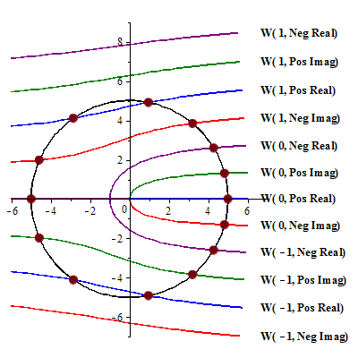
Figure 1: Solution in w-plane. $W(k,$ray$)$ means branch $k$ image of axial ray.

As an illustration, suppose that $R=5$. We will start with approach A, and observe that it reproduces the textbook solution. Figure 1 shows the $w$-plane. The circle $|w|=5$ is shown, along with maps of the real and imaginary axes as transformed by the Lambert W function. Various branches of the Lambert W function have been shown, for branch numbers 1 to -1 (using the conventional definitions of branch numbers from Corless, et al [13]). Only the branch numbers 1, 0 and -1 intersect the circle $|w|=5$. The first quadrant of figure 1, for $u>0$ and $v>0$, is readily seen to be equivalent to the textbook diagram, with the $u$ and $v$ axes flipped. Compare for instance figure 4.11 of Bransden and Joachain [3]; the authors, in their figure, use symbols $\xi$ for $v$, $\eta$ for $u$, and $\gamma$ for $R$. Their $\gamma=5$ curve shows the four bound state solutions, two even states and two odd states, as visible in the first quadrant of our figure 1.

Now, what happens if instead we use approach B to look at the solution for the $R=5$ example, working in the $z$-plane? Instead of the circle $P:\,|w|=5$ in the $w$-plane we have its transform $Q$ under the map $z=we^{w}$, which gives a closed curve in the $z$-plane, with multiple loops around the origin. We are interested in the places where that curve crosses one of the axes, since those are the possible solutions of the finite square well problem. Figures 2 to 5 show that curve, the whole of the $Q$ curve in figure 2, with magnifications in figures 3 to 5 to exhibit the fine details.

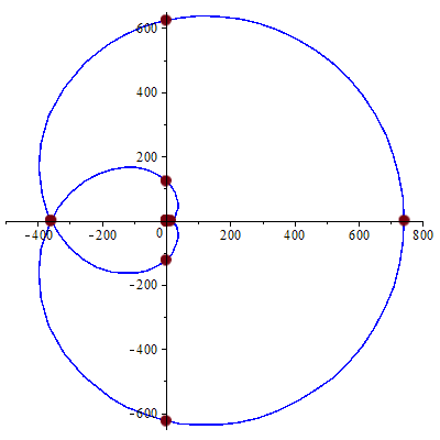
Figure 2: Solution in $z$-plane.

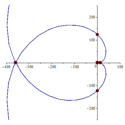
Figure 3: Solution in $z$-plane, magnified.

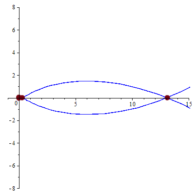
Figure 4: Solution in $z$-plane, magnified.

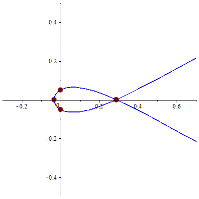
Figure 5: Solution in $z$-plane, magnified.

The $Q$ curve crosses the axes 14 times, counting multiplicities, ie crossings at the same coordinates but with different trajectories. Those correspond to the 14 solutions, the circle intersections in figure 1, of the problem visualized in the $w$-plane. To express those solutions in terms of the phase $\theta$ of the $w$ variable, write $w=R\,\mathrm{exp}(i\theta)$. Then the solutions (the phase angle $\theta$ parameter values when the curve $Q$ crosses one of the axes) are: x-axis crossings at $\theta=$ 0.000, 0.546, 1.377, 2.179, 3.142, 4.105, 4.906, 5.737, and y-axis crossings at $\theta=$ 0.264, 0.875, 2.735, 3.548, 5.408, 6.019.

To obtain the solutions in the first quadrant, that is with $u$ and $v$ required to be positive, we can simply restrict the $\theta$ phase to be between 0 and $\pi/2$, and exclude the case $\theta=0$ as not being physical. That produces the standard textbook results.

As one can see the Lambert W function, considered as a mapping between two planes, provides a visualization of the solution of the finite square well problem in terms of simple geometric objects: the real and imaginary axes, and circles around the origin. The area of the circle around the origin corresponds to the dimensions of the finite square well, and is proportional to the square of the strength parameter, that is, to the depth of the well and to the square of its linear dimension; in symbols, $R^{2}\sim V_{0}L^{2}$. The proportionality constant is $2m/{\hbar}^{2}$, and the units of that constant cancel the units of $V_{0}L^{2}$, resulting in $R^{2}$, and hence $R$, being unitless.

3 Discussion

The Lambert W description of the finite square well problem is best visualized as a conformal map between two complex planes, produced by the mapping $w\to z=w\,e^{w}$, the Lambert W function being the multi-branch inverse of that mapping.

The axial rays in the $z$-plane map to the Lambert W lines in the $w$-plane, whose intersections with the circle of radius $R$ about the origin give the solutions to the FSW problem. Alternatively, the circle of radius $R$ about the origin in the $w$-plane maps to a multi-loop closed curve in the $z$-plane, whose intersections with the axial rays also give the solutions to the FSW problem. Thus one may approach the problem situation working in either the $w$-plane (as is traditional), or in the $z$-plane – the choice of plane being determined by the convenience of other aspects of the particular problem which may be simpler in one or the other of those representations.

This technique bears some similarities to the method used in [15] to determine the fringing fields of a parallel plate capacitor.

Because the mapping is conformal, the angles between the circle in figure 1 and the various Lambert W lines are equal to the angles of the corresponding intersections in figure 2 of the multi-loop image of the circle and the axial rays. That suggests some possibilities for design of materials to be sensitive to slight changes in their environment, and leads back to the topic of the quantum well infrared photodetector (QWIP) with which we introduced this paper.

It is worth noting that the finite square well is “realistic” despite its simplicity, and continues to find use in contemporary research. For instance, Deshmukh, et al [16] use a 3-dimensional radial finite square well model to characterize the attosecond-scale time delays of the photoionization of an atom of Xenon trapped within a C60 fullerine molecule. Kocabas, et al [17], in a study of mathematical models for metal-insulator-metal waveguides, note (pages 13-14 of their paper) that there is a close relationship between the one-dimensional Schrödinger equation and the electromagnetic wave equation in layered media, and mention several ideas for investigation. They write “It is intriguing to ask whether such studies [of FSW solutions and their relationship to changes in reflection spectra of wells] could be useful in optics for the investigation of the effects of material interfaces”. Thus there is plenty of opportunity to do interesting work even with as old and familiar a topic as the finite square well.

There is a relationship of the solutions of the finite square well to the quadratix of Hippias, which is the solutions in the $(x,y)$ plane of the equation $x=y\,\mathrm{cot}\,y$. You can flip the axes or make translations to get other similar expressions of the relationship between the two variables. See Corless, et al [13], page 344.

The quadratix of Hippias can be used to solve various problems, such as the trisection of an arbitrary angle. Harper and Driskell [18] have an enjoyable description of construction of the quadratix, using interactive software for geometric constructions, and show how to use the quadratix to multiply an angle by any factor which can be expressed as a ratio of the lengths of two straight lines. That raises the entertaining possibility that one could perhaps present quantum mechanics in the language of Euclidean geometry. Physics textbooks could return to the geometric methods utilized by Sir Isaac Newton in his Principia! That is a somewhat lighthearted suggestion, essentially an entertainment, but it also represents a serious alternative view – and we may gain new insights. Quantum mechanics is already often described with a visual, diagrammatic language.

We anticipate there may be other interesting aspects of this geometric-analytic solution technique, for future exploration.

4 Conclusion

We have presented a solution of the quantum mechanics problem of the allowable energy levels of a bound particle in a 1-dimensional finite square well potential. The solution is a “geometric-analytic” technique utilizing the Lambert W function. The solutions can be represented in either of two domains, and a representation in the transformed domain has a particularly simple geometry. There are many opportunities to follow up. More work on this vibrant field of the application of the Lambert W function is anticipated.

SRV thanks King’s University College for their generous support.

References

- [1] Harald Schneider, Hui Chun Liu, Quantum Well Infrared Photodetectors: Physics and Applications, Springer, 2007.
- [2] P. Harrison, Quantum Wells, Wires and Dots: Theoretical and Computational Physics of Semiconductor Nanostructures, 3rd edition, Wiley, 2009.
- [3] B. H. Bransden, C. J. Joachain, Introduction to Quantum Mechanics, 2nd edition, Prentice-Hall, 2000.
- [4] E. E. Burniston, C. E. Siewert, “The use of Riemann problems in solving a class of transcendental equations”, Proceedings of the Cambridge Philosophical Society, vol 73 (1973), pp 111-118.
- [5] C. E. Siewert, E. E. Burniston, “Exact Analytical Solutions of ”, Journal of Mathematical Analysis and Applications, vol 43 (1973), pp 626-632.
- [6] C. E. Siewert, “Explicit results for the quantum-mechanical energy states basic to a finite square-well potential”, Journal of Mathematical Physics, vol 19, no 2 (February 1978), pp 434-435.
- [7] Prabasaj Paul, Daniel Nkemzi, “On the energy levels of a finite square-well potential”, Journal of Mathematical Physics, vol 41, no 7 (July 2000), pp 4551-4555.
- [8] David L. Aronstein, C. R. Stroud, Jr., “Comment on ‘On the energy levels of a finite square-well potential’”, Journal of Mathematical Physics, vol 41, no 12 (December 2000), pp 8349-8350.
- [9] R. Blümel, “Analytical solution of the finite quantum square-well problem”, Journal of Physics A, vol 38 (2005), pp L673-L678.
- [10] E. G. Anastasselou, N. I. Ioakimidis, “A generalization of the Siewert-Burniston method for the determination of zeros of analytic functions”, Journal of Mathematical Physics, vol 25, no 8 (August 1984), pp 2422-2425.
- [11] Eleni G. Anastasselou, Nokolaos I. Ioakimidis, “A New Approach to the Derivation of Exact Analytical Formulae for the Zeros of Sectionally Analytic Functions”, Journal of Mathematical Analysis and Applications, vol 112 (1985), pp 104-109.
- [12] Nikolaos I. Ioakimidis, “A Unified Riemann-Hilbert Approach to the Analytical Determination of Zeros of Sectionally Analytic Functions”, Journal of Mathematical Analysis and Applications, vol 129 (1988), pp 134-141.
- [13] R. M. Corless, G. H. Gonnet, D. E. G. Hare, D. J. Jeffrey, D. E. Knuth, “On the Lambert W function”, Advances in Computational Mathematics, vol 5 (1996), pp 329-359.
- [14] Frank Olver, et al (eds), NIST Handbook of Mathematical Functions, Cambridge, NIST, 2010. See page 111.
- [15] S. R. Valluri, D. J. Jeffrey, R. M. Corless, “Some applications of the Lambert W function to physics”, Canadian Journal of Physics, vol 78, no 9 (September 2000), pp 823-831.
- [16] P. C. Deshmukh, A. Mandal, A. S. Kheifets, V. K. Dolmatov, S. T. Manson, “Attosecond time delay in the photoionization of endohedral atoms : A new probe of confinement resonances”, Arxiv:1402.2348 (February 2014).
- [17] Sükrü Ekin Kocabas, Georgios Veronis, David A. B. Miller, Shanhui Fan, “Modal analysis and coupling in metal-insulator-metal waveguides”, Physical Review B, vol 79 (2009), article 035120.
- [18] Suzanne Harper, Shannon Driskell, “An Investigation of Historical Geometric Constructions”, Loci, August 2010.