Spaghetti prediction: A robust method for forecasting short time series

Abstract

A novel method for predicting time series is described and demonstrated. This method inputs time series data points and outputs multiple “spaghetti” functions from which predictions can be made. Spaghetti prediction has desirable properties that are not realized by classic autoregression, moving average, spline, Gaussian process, and other methods. It is particularly appropriate for short time series because it allows asymmetric prediction distributions and produces prediction functions which are robust in that they use multiple independent models.

I Motivation

Televised hurricane forecasts often feature plots that appear as multiple strands of cooked spaghetti tossed on a plate. Such “spaghetti” plots indicate the hurricane path predicted by independent meteorological models. Similarly, the novel spaghetti time series prediction method described and demonstrated here develops independent spaghetti functions, each of which constitutes a model of given time series data.

II Description

Given time series points $(x_{i},y_{i})$ with $i=1,2,\ldots n$, the spaghetti functions are

$$f_{i}(x)=a_{i}+b_{i}x+\sum_{k}A_{ik}\mathrm{e}^{(x-x_{k})^{2}/(2\sigma_{i}^{2})},$$ (1)

where $k$ is an index over the points with point $i$ left out, $a_{i}+b_{i}x$ is the least-squares line of the $(x_{k},y_{k})$, $A_{ik}$ and $\sigma_{i}$ are chosen to minimize

$$\sum_{k}[y_{k}-f_{i}(x_{k})]^{2}+\lambda_{i}\int_{-\infty}^{\infty}\left(\frac{\mathrm{d}^{2}f_{i}(x)}{\mathrm{d}x^{2}}\right)^{2}\mathrm{d}x,$$

and $\lambda_{i}$ is positive and minimizes $|y_{i}-f_{i}(x_{i})|$.

Comments on this description are as follows:

1. Each spaghetti function is developed with one time series point left out, so there are $n$ functions. Each function is the least squares line of the $n-1$ points plus a weighted linear combination of Gaussian (i.e., normal distribution) basis functions or kernels, where each kernel is centered on one of the points and has the same variance.

2. Each spaghetti function has its kernel weights and kernel variance determined so that deviation plus the product of a positive constant and roughness is minimized. Deviation has the classic sum squared difference from the points definition, and roughness has the classic integrated squared second derivative definition [MacKay, 2003; Gustafson et al., 2007].

3. If $\lambda_{i}$ is nearly zero, then deviation minimization dominates, and the spaghetti function nearly intersects the $n-1$ points. If $\lambda_{i}$ is nearly infinite, then roughness mnimization dominates, and the spaghetti function is nearly the least squares line of the $n-1$ points. Thus $\lambda_{i}$ controls the function shape in a manner consistent with classic (i.e., standard or well-known) regularization methods [MacKay, 2003; Gustafson et al., 2011].

4. The $\lambda_{i}$ for each spaghetti function is determined so as to best predict the left out point, i.e., it is such that the absolute difference between the function and the left out point is minimized. Thus the shape of each spaghetti function is adjusted so that it predicts the left out point with least error. This method for developing multiple independent models is novel in that (to our knowledge) it has not been reported in the technical literature.

Two classic functions may be compared with the spaghetti functions:

1. The least squares line of all of the points: $g(x)=a+bx$, where $a$ and $b$ minimize $\sum_{i}[y_{i}-g(x_{i})]^{2}$. Note that $g(x)$ is the spaghetti function of all the points as $\lambda$ approaches infinity and that it is also the function of zero roughness that has least deviation.

2. The least rough interpolator of all the points: $h(x)=a+bx+\sum_{i}A_{i}\exp[(x-x_{i})^{2}/(2\sigma^{2})]$, where the $A_{i}$ are such that $h(x_{i})=y_{i}$ and $\sigma$ is such that $\int_{-\infty}^{\infty}\left(\frac{\mathrm{d}^{2}h(x)}{\mathrm{d}x^{2}}\right)^{2}\mathrm{d}x$ is minimized. Note that $h(x)$ is the spaghetti function of all the points as $\lambda$ approaches zero and that it is also the function of zero deviation that has least roughness.

III Demonstration

Figure 1 shows seven time series points, the seven spaghetti functions $f_{i}(x)$, and the mean $\mu(x)$ of the spaghetti functions. As described above, each spaghetti function has its deviation-roughness tradeoff optimized so that it predicts its corresponding left out point with least error. The spaghetti functions constitute multiple independent models of the time series data and enable robust prediction at any time. In general, the distribution of spaghetti function predictions at any time is not symmetric. Fiigure 1 indicates this asymmetry in that that the mean of the spaghetti functions differs from the median function (i.e., the middle function). Asymmetric prediction distributions are particularly realistic for short time series.

Figure 1: Seven time series points (dots), the seven spaghetti functions $f_{i}(x)$ (dotted curves), and the mean $\mu(x)$ (solid curve) of the spaghetti functions. Note that the distribution of spaghetti functions is asymmetric in that the median or middle spaghetti function differs from $\mu(x)$.

Figure 2 shows the seven points, $\mu(x)$, $\mu(x)+s(x)$, and $\mu(x)-s(x)$, where $s(x)$ is the standard deviation of the spaghetti functions.  The standard deviation of the spaghetti functions should be small near the points and large away from them, because prediction should be more accurate near the points. The figure shows that this behavior is realized.

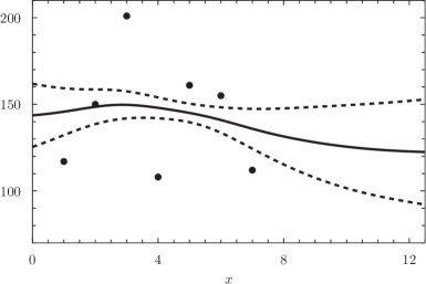
Figure 2: The seven points (dots), $\mu(x)$ (solid curve), $\mu(x)+s(x)$ (dashed curve), and $\mu(x)-s(x)$ (dashed curve), where $s(x)$ is the standard deviation of the spaghetti functions. Note that $s(x)$ is small near the points and large away from them.

Figure 3 shows the seven points and three functions that characterize them: their least squares line $g(x)$, their least rough interpolator $h(x)$, and the mean of the spaghetti functions $\mu(x)$. The mean of the spaghetti functions should extrapolate to a line, because prediction should employ the simplest functional form far from the points. The figure illustrates this behavior, and it shows that the line is the least squares line of the points.

Figure 3: The seven points and three functions that characterize them:  their least squares line $g(x)$ (dotted curve), their least rough interpolator $h(x)$ (dashed curve), and the mean of the spaghetti functions $\mu(x)$ (solid curve). Note that $\mu(x)$ extrapolates to $g(x)$.

IV Discussion

Spaghetti prediction could be compared with numerous time series prediction methods on various real or synthetic data sets. However, as is well known, data can almost always be found or synthesized (there are only trivial exceptions) to show that a given prediction method outperforms competing methods in accord with given criteria [Duda et al., 2000; Poggio et al. 2004]. Thus the focus of comparison should be on the properties of the prediction methods.

A wide range of time series prediction methods [Anava et al., 2013] are in effect realizations of Gaussian processes that correspond to specific choices of a covariance function [Rasmussen et al., 2007]. Classic methods, including autoregressive and moving average methods and their various combinations and extensions, e.g., the well-known Box-Jenkins methods, are such in-effect realizations, as are various spline methods, e.g., smoothing and B-splines [Brockwell, et al. 2009]. However, spaghetti prediction is not a realization of a Gaussian process. In a Gaussian process the dependent variable has a Gaussian probability density function (pdf) at any given time, and thus the pdf is symmetric and the mean, median, and mode are identical. In spaghetti prediction the pdf of the dependent variable at any given time does not have this constraint. This property is important for short time series (i.e., series that have a small number of given points), which are likely to be characterized by asymmetric prediction distributions.

Spaghetti prediction has other properties that contrast with Gaussian process methods. A Gaussian process produces a single prediction function and a variance for this function at any time, but spaghetti prediction produces as many prediction functions as there are data points. Furthermore, each spaghetti function has the tradeoff between its roughness and its deviation from the data with one point left out optimized so as to predict the left out point with least error. In making this tradeoff, classic definitions of deviation and roughness are employed, and each spaghetti function has a classic form: the least squares line of the retained points plus a weighed sum of point-centered Gaussian kernels of the same variance.

Spaghetti prediction is particularly appropriate for short time series. In this case a robust method, i.e., a method that produces multiple independent predictions, is especially important. Also, as discussed above, the distribution of predictions is typically skewed for small data sets, and thus a method that permits an asymmetric distribution of predictions is particularly important. Spaghetti prediction, unlike Gaussian process methods, has these properties.

References

O. Anava, E. Hazan, S. Mannor, O. Shamir, “Online learning for time series prediction”, arXiv: 1302.6927v1, 2013.

P. Brockwell, R. Davis, “Time series: theory and methods”, Springer, 2009.

R. Duda, P. Hart, D. Stork, “Pattern classification”, Wiley, 2000.

S. Gustafson, D. Parker, “Cardinal interpolation”, IEEE Trans. PAMI 29: 1538 – 1545, 2007.

S. Gustafson, A. Hillier, “A probability density for modeling unknown physical processes”, arXiv: 1104.3992, 2011.

D. MacKay, “Information theory, inference, and learning algorithms”, Cambridge, 2003.

T. Poggio, R. Rifkin, S. Mukherjee, P. Niyogi, “General conditions for predictivity in learning theory”, Nature 428: 419 – 422, 2004.

C. Rasmussen, C. Williams, “Gaussian processes for machine learning”, MIT press, 2006.