Nonexistence of entangled continuous-variable Werner states with positive partial transpose

Abstract

We address an open question about the existence of entangled continuous-variable (CV) Werner states with positive partial transpose (PPT). We prove that no such state exists by showing that all PPT CV Werner states are separable. The separability follows by observing that these CV Werner states can be approximated by truncating the states into a finite-dimensional convex mixture of product states. In addition, the constituents of the product states comprise a generalized non-Gaussian measurement which gives, rather surprisingly, a strictly tighter upper bound on quantum discord than photon counting. These results uncover the presence of only negative partial transpose entanglement and illustrate the complexity of more general non-classical correlations in this paradigmatic class of genuine non-Gaussian quantum states.

I Introduction

Convex mixtures of a maximally entangled state and a maximally mixed state of two two-level quantum systems (qubits) represent undoubtedly the most important mixed test states in quantum information theory. These states, commonly called Werner states Werner_89 , combine quantum entanglement and classical noise in a simple way that allows for the testing of quantum information criteria, concepts and protocols in the mixed-state domain using analytical tools. Originally developed as an example of an entangled state which admits a local-realistic model Werner_89 , i.e., a state which does not violate any Bell-type inequalities, it was shown later that suitable Werner states may exhibit hidden nonlocality Gisin_96 and that a Werner state admitting a local-realistic model can exhibit nonlocality in the multicopy scenario Peres_96a . In the context of separability, Werner states have been used to demonstrate that separability criteria based on positive partial transposition Peres_96b or majorization Nielsen_01 are strictly stronger than entropic ones. Furthermore, Werner states prove to be suitable initial states for entanglement distillation Bennett_96 . Interestingly, not only entangled Werner states play an important role in quantum information; it turns out that separable Werner states can carry non-classical correlations, known as quantum discord Olivier_02 , which can serve as an alternative resource for quantum technology, e.g., in quantum illumination Weedbrook_13 .

All aforementioned applications relate to the two-qubit Werner states. An important test state is also obtained when we extend the Werner state to systems with an infinite-dimensional Hilbert space, such as optical modes. A two-mode analogue of the Werner state, the so called continuous-variable (CV) Werner state, for two modes $A$ and $B$ is defined as Mista_02

$$\rho_{p}=p\sigma+(1-p)\tau,\quad 0\leq p\leq 1.$$ (1)

Here

$$\sigma=\left(1-\lambda_{1}^{2}\right)\sum_{m,n=0}^{\infty}\lambda_{1}^{m+n}|m,m\rangle\langle n,n|$$ (2)

is the two-mode squeezed vacuum state, where $|m,n\rangle\equiv|m\rangle_{A}\otimes|n\rangle_{B}$ with $|k\rangle_{j}$ being the $k$-th Fock state of mode $j$, with $\lambda_{1}=\tanh r$ and squeezing parameter $r$, and

$$\tau=\left(1-\lambda_{2}^{2}\right)^{2}\sum_{m,n=0}^{\infty}\lambda_{2}^{2(m+n)}|m\rangle\langle m|\otimes|n\rangle\langle n|$$ (3)

is the tensor product of two identical thermal states characterized by the parameter $\lambda_{2}=\tanh s$. For $r=s$ and in the strong squeezing limit $r\rightarrow\infty$, the state (1) represents a direct analogy of the original two-qubit Werner state by approaching a convex mixture of a maximally entangled state and a maximally mixed state in an infinite-dimensional Hilbert space.

The CV Werner state (1) is a simple mixed non-Gaussian state and therefore proves to be an excellent tool for investigating many concepts in quantum information in the mixed-state non-Gaussian scenario. This involves analyses of separability, teleportation and violation of discrete-variable Bell inequalities Mista_02 , as well as for non-classical correlations beyond entanglement Tatham_12 . Besides, CV Werner states have been studied also from the point of view of violation of the CV Bell inequalities Borges_12 , quantification of non-Gaussian entanglement by negativity Lund_08 ; Rodo_08 or optimality of Gaussian attacks in CV quantum key distribution Lund_08 . Despite considerable progress in understanding many aspects of the CV Werner states, their basic separability properties are still not fully known. Analysis of their separability has been performed using the positive partial transposition (PPT) criterion Peres_96b . The criterion says that any two-mode separable density matrix $\rho$ has a positive partial transpose $\rho^{T_{A}}$, which is a matrix with entries

$$\langle m,\mu|\rho^{T_{A}}|n,\nu\rangle\equiv\langle n,\mu|\rho|m,\nu\rangle.$$ (4)

From the PPT criterion it then follows that a quantum state is entangled if its density matrix has a negative partial transpose (NPT). The CV Werner state (1) is exceptional because its NPT region can be found analytically Mista_02 . However, this region may not contain all entangled CV Werner states since PPT entangled states may also exist PHorodecki_97 . In Ref. Mista_02 a set of all PPT CV Werner states and a nontrivial proper subset of separable states have been found. Therefore, there still exist PPT CV Werner states for which the separability properties are not known. In particular, it is unknown whether PPT entangled CV Werner states exist.

In the subsequent sections we answer this existence question in the negative. First, we prove that any PPT $N$-dimensional truncation of the CV Werner state (1) is separable for any finite $N$. We then show that any PPT CV Werner state can be approximated in the trace-norm by a sequence of its truncated separable counterparts, which implies its separability. The separability of the PPT truncated $N\times N$ CV Werner states is demonstrated by finding explicitly their decomposition into a convex mixture of pure product states, which is inspired by the method Kraus_00 developed for simpler $2\times N$ quantum systems. Contrary to intuition, the projectors onto the constituents of the product states comprise a generalized non-Gaussian measurement which yields, for a particular example of the partial transpose of a specific PPT CV Werner state, a strictly tighter upper bound on quantum discord than photon counting.

The first result of the present paper closes a long-standing open problem about the existence of PPT CV entangled Werner states. The second result shows that more sophisticated non-Gaussian measurements are needed to optimally extract non-classical correlations from non-Gaussian quantum states on infinite-dimensional Hilbert state spaces.

The paper is organized as follows. In Section II we prove the separability of all PPT finite-dimensional truncations of CV Werner states, while Section III is dedicated to the proof of the separability of any PPT CV Werner state. In Section IV we show that photon counting does not minimize quantum discord for a certain family of partially transposed CV Werner states. Finally, Section V contains conclusions.

II Finite dimensions

At the outset we will investigate the separability of PPT states obtained by truncating the CV Werner states (1) onto a finite-dimensional Hilbert space. For two optical modes $A$ and $B$ the truncation is defined as

$$\rho_{p,N}=\mathcal{N}_{p,N}\left[p\sigma_{N}+(1-p)\tau_{N}\right],\quad 0\leq p\leq 1.$$ (5)

Here,

$$\sigma_{N}=\left(1-\lambda_{1}^{2}\right)\sum_{m,n=0}^{N-1}\lambda_{1}^{m+n}|m,m\rangle\langle n,n|$$ (6)

is the truncated two-mode squeezed vacuum state, and

$$\tau_{N}=\left(1-\lambda_{2}^{2}\right)^{2}\sum_{m,n=0}^{N-1}\lambda_{2}^{2(m+n)}|m\rangle\langle m|\otimes|n\rangle\langle n|$$ (7)

is the tensor product of two identical truncated thermal states. The normalization factor is given by

$$\mathcal{N}_{p,N}=\left[p\left(1-\lambda_{1}^{2N}\right)+\left(1-p\right)\left(1-\lambda_{2}^{2N}\right)^{2}\right]^{-1}.$$ (8)

There are two PPT regions for the state $\rho_{p,N}$ which can be distinguished depending on the relation between parameters $\lambda_{1}$ and $\lambda_{2}$ Mista_02 .

i) For $\lambda_{1}>\lambda_{2}^{2}$ the state (5) is PPT if and only if

$$p\leq\frac{1}{1+\frac{(1-\lambda_{1}^{2})}{(1-\lambda_{2}^{2})^{2}}\left(\frac{\lambda_{1}}{\lambda_{2}^{2}}\right)^{2N-3}}\equiv p_{N}.$$ (9)

ii) For $\lambda_{1}\leq\lambda_{2}^{2}$ the state (5) is PPT if and only if

$$p\leq p_{N=2}\equiv p_{2}.$$ (10)

Note, that while region (ii) coincides with the region of PPT CV Werner states of infinite dimension Mista_02 , region (i) varies from the infinite case, but it approaches the region of infinite-dimensional PPT CV Werner states characterized by the condition $p=0$ Mista_02 in the limit of $N\rightarrow\infty$.

Let us start with an analysis of separability of the simple PPT boundary state ($\equiv\rho_{q,N}$) from region (ii) for which $\lambda_{1}=\lambda_{2}^{2}$ and

$$p=p_{2}=\frac{1-\lambda_{1}}{2}\equiv q.$$ (11)

According to the definition Werner_89 , a density matrix $\rho$ is separable if it can be written or approximated in the trace norm by the states of the form

$$\rho=\sum_{i}p_{i}\rho_{A}^{(i)}\otimes\rho_{B}^{(i)},\quad 0\leq p_{i}\leq 1,\quad\sum_{i}p_{i}=1,$$ (12)

where $\rho_{j}^{(i)}$ is a local density matrix of mode $j$. In order to investigate the separability of $\rho_{q,N}$ it is easier to analyze the simpler partially transposed state $\rho_{q,N}^{T_{A}}$, since the separability of one implies the separability of the other. From Eqs. (4) and (5) we get for the partially transposed state the expression

$$\rho_{q,N}^{T_{A}} = \mathcal{K}_{N}\sum_{m,n=0}^{N-1}\lambda^{m+n}\left(|n,m\rangle\langle m,n|+|m,n\rangle\langle m,n|\right),$$

where we set $\lambda_{1}=\lambda$ and

$$\mathcal{K}_{N}=\frac{\left(1-\lambda^{2}\right)\left(1-\lambda\right)}{2\left(1-\lambda^{N}\right)\left(1-\lambda^{N+1}\right)}$$ (14)

is the normalization factor. Here, and in what follows, we will sometimes use the unnormalized state $\tilde{\rho}_{q,N}^{T_{A}}=\rho_{q,N}^{T_{A}}/\mathcal{K}_{N}$ for brevity.

Let us first start our separability analysis with the simplest case $N=2$. Here, PPT implies separability and thus the state $\tilde{\rho}_{q,2}^{T_{A}}$ must be separable. Making use of a method developed in Kraus_00 we can find explicitly a decomposition of the state into a convex mixture of pure product states.

The construction given in Kraus_00 involves finding and subtracting product vectors from a state $\rho$ on the space $\mathbb{C}^{2}\otimes\mathbb{C}^{N}$ such that $\rho$ and $\rho^{T_{A}}$ remain positive. If enough product vectors exist so that $\rho$ reduces to zero then the state is obviously separable. The first step in finding such a decomposition for $N=2$ is to calculate $\tilde{r}=\text{rank}(\rho)+\text{rank}(\rho^{T_{A}})$. If $\tilde{r}\leq 3N=6$ then finding the product vectors involve calculating the roots of a polynomial. If, however, $\tilde{r}>6$ then one can always subtract product vectors from $\rho$ to reduce its rank such that $\tilde{r}\leq 6$ without affecting positivity. In particular, one must find vectors $|e,f\rangle$ in the range of $\rho$ such that $|{e^{*}},f\rangle$ lies in the range of $\rho^{T_{A}}$, where $|{e^{*}}\rangle$ denotes complex conjugation of $|e\rangle$. Once $\tilde{r}\leq 6$ we must then solve a polynomial to find the remaining product states in the decomposition.

For the specific state $\tilde{\rho}_{q,2}$ we first subtract $|0,0\rangle+\lambda|1,1\rangle$ to reduce its rank by one, such that $\tilde{r}=6$. It then remains to find the roots $\alpha$ of the polynomial $\text{det}[M(\alpha,{\alpha^{*}})]$ for the $(2\times 2)$ matrix $M$ given by

$$M(\alpha,{\alpha^{*}})=\left(\begin{array}[]{c}\alpha\langle\psi_{1}|0\rangle+\langle\psi_{1}|1\rangle\\ {\alpha^{*}}\langle\psi_{2}|0\rangle+\langle\psi_{2}|1\rangle\end{array}\right),$$ (15)

where $|\psi_{1}\rangle$ and $|\psi_{2}\rangle$ are the $(4\times 1)$ basis vectors for the one-dimensional kernels of $\tilde{\rho}_{q,2}$ and $\tilde{\rho}^{T_{A}}_{q,2}$, respectively, and $\langle\psi_{j}|i\rangle=\sum_{l=0}^{1}\psi_{il}^{(j)\ast}\langle l|$ with $\langle i,l|\psi_{j}\rangle=\psi_{il}^{(j)}$. We then arrive at the polynomial equation $\alpha{\alpha^{*}}\sqrt{\lambda}-1=0$ which we solve to find four more product vectors of the form

$$|e,f\rangle=(\alpha|0\rangle_{A}+|1\rangle_{A})\otimes\sum_{k=0}^{1}f_{k}|k\rangle_{B}.$$ (16)

Here the vector $|f\rangle$ is found by calculating the kernel of matrix $M$, i.e., $M(\alpha,{\alpha^{*}})\vec{f}=0$ with $\vec{f}=(f_{0},f_{1})^{T}$, where $f_{i}=\langle i|f\rangle$, $i=0,1$. After rewriting in a more compact form, the original state can be expressed as $\tilde{\rho}_{q,2}^{T_{A}}=D^{(2)}$, where

$$D^{(2)} = \sum_{n=0}^{1}\lambda^{2n}|n,n\rangle\langle n,n|+\frac{1}{4}\sum_{n=0}^{3}|q_{n},q_{n}\rangle\langle q_{n},q_{n}|,$$

and $|q_{n}\rangle=|0\rangle+e^{i\frac{\pi n}{2}}\sqrt{\lambda}|1\rangle$.

Moving now to the case of $N>2$, we cannot directly apply the previous method as it has been developed for only $2\times N$ systems Kraus_00 . Nevertheless, the structure of the decomposition for $N=2$ can still inspire us to find a similar separable decomposition for the state $\tilde{\rho}_{q,N}^{T_{A}}$. In particular, we will show that $\tilde{\rho}_{q,N}^{T_{A}}=D$, for $N>2$, where

$$D=\sum_{n=0}^{N-1}\lambda^{2n}|n,n\rangle\langle n,n|\\ +\frac{1}{N^{N-1}}\sum_{n_{1},\ldots,n_{N-1}=0}^{N-1}|q_{\vec{n}},q_{\vec{n}}\rangle\langle q_{\vec{n}},q_{\vec{n}}|,$$ (18)

with $\vec{n}=(n_{1},\ldots,n_{N-1})$ and $|q_{\vec{n}}\rangle=|0\rangle+\sum_{j=1}^{N-1}e^{i\frac{2\pi}{N}n_{j}}\lambda^{j/2}|j\rangle$.

We find the matrix elements $D_{jk,lm}=\langle j,k|D|l,m\rangle$ of the decomposition (18) as

$$D_{jk,lm} = \lambda^{2j}\delta_{kj}\delta_{lj}\delta_{mj}+\frac{1}{N^{N-1}}(\sqrt{\lambda})^{j+k+l+m}$$ (19)

$$\times\sum_{n_{1},\ldots,n_{N-1}=0}^{N-1}e^{i\frac{2\pi}{N}(n_{j}+n_{k}-n_{l}-n_{m})},$$

where $n_{0}\equiv 0$. Making use of the simple relation

$$\sum_{n_{1},\ldots,n_{N-1}=0}^{N-1}e^{i\frac{2\pi}{N}(n_{j}-n_{k})}=N^{N-1}\delta_{jk}$$ (20)

to find

$$\sum_{n_{1},\ldots,n_{N-1}=0}^{N-1}e^{i\frac{2\pi}{N}(n_{j}+n_{k}-n_{l}-n_{m})}=\\ N^{N-1}\left(\delta_{jl}\delta_{km}+\delta_{jm}\delta_{kl}-\delta_{jk}\delta_{jl}\delta_{jm}\right),$$ (21)

we arrive at

$$D_{jk,lm}=\lambda^{j+k}(\delta_{jl}\delta_{km}+\delta_{jm}\delta_{kl}).$$ (22)

Note that Eq. (21) is only valid for $N>2$. Since (22) are just the matrix elements $(\rho_{q,N}^{T_{A}}/\mathcal{K}_{N})_{jk,lm}$, we have shown that the state (II) really can be expressed as a convex mixture of product states (12), which reads explicitly as

$$\rho_{q,N}^{T_{A}}=\mathcal{K}_{N}D,$$ (23)

where the operator $D$ is given in Eq. (18), and therefore the state is separable. Consequently, the original truncated CV Werner state $\rho_{q,N}$ can be expressed as the following convex mixture of product states

$$\rho_{q,N}=\mathcal{K}_{N}D^{T_{A}},$$ (24)

and therefore it is also separable.

We will now investigate the separability of the state $\rho_{p,N}$ for all other values of $p$ and show that it is in fact separable when the inequalities (9) and (10) are satisfied. In other words, for any PPT region the truncated CV Werner state is separable. Our previous derivation of the separable decomposition for $\rho_{q,N}^{T_{A}}$ will prove useful to show this.

Firstly we rewrite the state (5) as

$$\rho_{p,N}=\alpha\sum_{m,n=0}^{N-1}\lambda_{1}^{m+n}\left(|m,m\rangle\langle n,n|+|m,n\rangle\langle m,n|\right)\\ +\sum_{m,n=0}^{N-1}\left[\beta\lambda_{2}^{2(m+n)}-\alpha\lambda_{1}^{m+n}\right]|m,n\rangle\langle m,n|,$$ (25)

with $\alpha=p(1-\lambda_{1}^{2})\mathcal{N}_{p,N}$ and $\beta=(1-p)(1-\lambda_{2}^{2})^{2}\mathcal{N}_{p,N}$. Now the first sum of (25) is equal to $\tilde{\rho}_{q,N}\equiv\rho_{q,N}/\mathcal{K}_{N}$ and can be replaced by $D^{T_{A}}$ from (18) with $\lambda=\lambda_{1}$. After further rewriting it follows that the state is separable if

$$\sum_{m\neq n=0}^{N-1}\left[\beta\lambda_{2}^{2(m+n)}-\alpha\lambda_{1}^{m+n}\right]|m,n\rangle\langle m,n|\geq 0,$$ (26)

which is equivalent to the condition $\beta\lambda_{2}^{2(m+n)}-\alpha\lambda_{1}^{m+n}\geq 0$ for $m\neq n$. This is identical to the condition

$$p\leq\frac{1}{1+\frac{(1-\lambda_{1}^{2})}{(1-\lambda_{2}^{2})^{2}}\left(\frac{\lambda_{1}}{\lambda_{2}^{2}}\right)^{m+n}}.$$ (27)

For the region $\lambda_{1}\leq\lambda_{2}^{2}$, the RHS of (27) is minimal when $m+n=1$ and therefore the state is separable when

$$p\leq p_{2}=\frac{1}{1+\frac{(1-\lambda_{1}^{2})}{(1-\lambda_{2}^{2})^{2}}\frac{\lambda_{1}}{\lambda_{2}^{2}}},$$ (28)

which, according to Eq. (10), is the same condition for positive partial transposition. In particular, on the boundary $\lambda_{1}=\lambda_{2}^{2}$, the inequality simplifies to $p\leq q=\frac{1-\lambda_{1}}{2}$. Finally, for the case $\lambda_{1}>\lambda_{2}^{2}$, the RHS of (27) is minimized when $m+n$ is maximal. This occurs when $m+n=2N-3$ and hence we arrive at inequality (9) given by

$$p\leq\frac{1}{1+\frac{(1-\lambda_{1}^{2})}{(1-\lambda_{2}^{2})^{2}}\left(\frac{\lambda_{1}}{\lambda_{2}^{2}}\right)^{2N-3}}.$$ (29)

Since this region of $p$ accommodates all PPT states for $\lambda_{1}>\lambda_{2}^{2}$, there is no room left for PPT entangled states.

III Infinite dimensions

As we have just seen, for finite $N$ the truncated CV Werner state $\rho_{p,N}$ is never entangled when its partial transposition is positive. In fact, the same statement holds also for the infinite-dimensional CV Werner state $\rho_{p}$ in Eq. (1), as we will show now.

Similarly to Eq. (25), we can decompose the state $\rho_{p}$ as

$$\rho_{p} = \frac{\alpha^{\prime}}{\mathcal{J}}\bar{\rho}_{q}+\sum_{m\neq n=0}^{\infty}\left[\beta^{\prime}\lambda_{2}^{2(m+n)}-\alpha^{\prime}\lambda_{1}^{m+n}\right]|m,n\rangle\langle m,n|$$ (30)

$$+\beta^{\prime}\sum_{n=0}^{\infty}\lambda_{2}^{4n}|n,n\rangle\langle n,n|,$$

where $\mathcal{J}=(1-\lambda_{1})^{2}$, $\alpha^{\prime}=p(1-\lambda_{1}^{2})$, $\beta^{\prime}=(1-p)(1-\lambda_{2}^{2})^{2}$, and

$$\bar{\rho}_{q} = \mathcal{J}\left(\frac{\rho_{q}}{\mathcal{K}}-\sum_{n=0}^{\infty}\lambda_{1}^{2n}|n,n\rangle\langle n,n|\right),$$ (31)

where

$$\rho_{q} = \mathcal{K}\sum_{m,n=0}^{\infty}\lambda_{1}^{m+n}\left(|m,m\rangle\langle n,n|+|m,n\rangle\langle m,n|\right)$$

and $\mathcal{K}=(1-\lambda_{1}^{2})(1-\lambda_{1})/2$ is the normalization factor. Obviously, the state $\rho_{p}$ is separable if both the density matrix $\bar{\rho}_{q}$ as well as the first sum on the right-hand side of Eq. (30) are separable quantum states. As in the finite-dimensional case, the sum describes a separable quantum state if the inequality (27) is fulfilled. Hence, for $\lambda_{1}\leq\lambda_{2}^{2}$, the sum is a separable state if the inequality (28) is satisfied, while for $\lambda_{1}>\lambda_{2}^{2}$ the inequality (29) is replaced by $p=0$. These regions all agree with the PPT regions for the CV Werner state and therefore, for all PPT CV Werner states, the first sum on the right-hand side of Eq. (30) is always a separable quantum state. Consequently, if the density matrix (31) is a separable state for all $\lambda_{1}$, then all CV Werner states (1) with a positive partial transposition are separable.

Unfortunately, in the limit of $N\rightarrow\infty$, the product decomposition (24) for the state $\rho_{q,N}$ does not generalize straightforwardly and thus the separability of the density matrix (31) is not obvious. However, when the dimension of the Hilbert space is infinite, we can use the limit definition of separability Werner_89 ; Clifton_99 to prove the separability of the state $\bar{\rho}_{q}$, given in Eq. (31). According to the definition in Eisert_02 , a density matrix $\rho$ is separable if there exists a sequence $\{\rho_{n}\}_{n=1}^{\infty}$ of density matrices $\rho_{n}$ such that each $\rho_{n}$ can be expressed as a convex mixture of product states (12), and such that

$$\lim_{n\rightarrow\infty}\|\rho-\rho_{n}\|_{1}=0,$$ (33)

where $\|.\|_{1}$ is the trace norm.

It is again convenient to prove the separability of the partially transposed state $\bar{\rho}_{q}^{T_{A}}$. The candidate for the sequence of separable states approximating the state $\bar{\rho}_{q}^{T_{A}}$ in trace norm is the sequence of states

$$\bar{\rho}_{q,N}^{T_{A}} = \mathcal{J}_{N}\left(\frac{\rho_{q,N}^{T_{A}}}{\mathcal{K}_{N}}-\sum_{n=0}^{N-1}\lambda_{1}^{2n}|n,n\rangle\langle n,n|\right),$$ (34)

where $\mathcal{J}_{N}=[(1-\lambda_{1})/(1-\lambda_{1}^{N})]^{2}$, and $\mathcal{K}_{N}$ and $\rho_{q,N}^{T_{A}}$ are defined in Eqs. (14) and (23), respectively, where $\lambda$ is replaced with $\lambda_{1}$. In other words, the sequence $\{\rho_{n}\}_{n=1}^{\infty}$ in our case reads $\rho_{n}\equiv\bar{\rho}_{q,n+2}^{T_{A}}$, $n=1,2,\ldots$. Therefore, our goal is to verify the limit (33) for the Hermitian operator $\bar{\rho}_{q}^{T_{A}}-\rho_{n}$ with $\rho_{n}=\bar{\rho}_{q,N}^{T_{A}}$, where here, and in what follows, we use the label $N=n+2$ for simplicity. The trace norm of a Hermitian operator $X$ is defined as $\|X\|_{1}\equiv\mbox{Tr}\sqrt{X^{{\dagger}}X}$ Reed_72 and it is equal to the sum of the absolute values of the eigenvalues of the operator $X$ Vidal_02 . The operator $\bar{\rho}_{q}^{T_{A}}-\bar{\rho}_{q,N}^{T_{A}}$ has a block-diagonal form with $1\times 1$ blocks in the one-dimensional subspaces $\mathcal{H}^{(l)}$ spanned by the vectors $\{|l,l\rangle\}$, $l=0,1,2,\ldots$ and $2\times 2$ blocks in the two-dimensional subspaces $\mathcal{H}^{(j,k)}$ spanned by the vectors $\{|j,k\rangle,|k,j\rangle\,j>k\}$, $j,k=0,1,2,\ldots$. On each subspace $\mathcal{H}^{(j,k)}$ the operator $\bar{\rho}_{q}^{T_{A}}-\bar{\rho}_{q,N}^{T_{A}}$ has one zero eigenvalue and one nonzero eigenvalue of the form

$$e^{(jk)}=\left\{\begin{array}[]{ll}2(\mathcal{J}-\mathcal{J}_{N})\lambda^{j+k},&j,k=0,1,\ldots,N-1\\ 2\mathcal{J}\lambda^{j+k}\,,&\hbox{otherwise}\end{array}\right.$$ (35)

while on the subspace $\mathcal{H}^{(l)}$ it has one eigenvalue equal to

$$e^{(l)}=\left\{\begin{array}[]{ll}(\mathcal{J}-\mathcal{J}_{N})\lambda^{2l},&0\leq l\leq N-1\\ \mathcal{J}\lambda^{2l}\,,&N\leq l\end{array}\right.$$ (36)

where here and in what follows we set $\lambda_{1}=\lambda$ for brevity. Hence, the sought trace norm reads as

$$\|\bar{\rho}_{q}^{T_{A}}-\bar{\rho}_{{q},N}^{T_{A}}\|_{1} = (\mathcal{J}_{N}-\mathcal{J})\left(\sum_{k=0}^{N-1}\lambda^{2k}+2\sum_{j>k=0}^{N-1}\lambda^{j+k}\right)+\mathcal{J}\left(\sum_{k=N}^{\infty}\lambda^{2k}+2\sum_{j=N}^{\infty}\sum_{k=0}^{N-1}\lambda^{j+k}+2\sum_{j>k=N}^{\infty}\lambda^{j+k}\right),$$ (37)

where $\mathcal{J}_{N}$ is defined below Eq. (34), and where we have used the inequality $\mathcal{J}\leq\mathcal{J}_{N}$. The geometric series on the right-hand side of the latter equation can be summed, and after some algebra becomes

$$\|\bar{\rho}_{q}^{T_{A}}-\bar{\rho}_{q,N}^{T_{A}}\|_{1} = 4\lambda^{N}-2\lambda^{2N}.$$ (38)

Returning back to the original label $n$ by substituting $N=n+2$ we get

$$\|\bar{\rho}_{q}^{T_{A}}-\rho_{n}\|_{1} = 4\lambda^{n+2}-2\lambda^{2(n+2)}.$$ (39)

As $0\leq\lambda<1$, the right-hand side forms the $n$th element of a convergent series and therefore in the limit $n\rightarrow\infty$ it vanishes, i.e.,

$$\lim_{n\rightarrow\infty}\|\bar{\rho}_{q}^{T_{A}}-\rho_{n}\|_{1}=0.$$ (40)

The density matrix $\bar{\rho}_{q}^{T_{A}}$ is therefore separable and it can be expressed as a continuous convex mixture of product states Holevo_05 . Linearity of partial transposition preserves the structure of the state and hence also the original density matrix $\bar{\rho}_{q}$ is separable. Consequently, all PPT CV Werner states are separable as we set out to prove.

IV Photon counting does not minimize discord

The simplicity of CV Werner states makes them a perfect test bed for the challenging analysis of correlations in CV non-Gaussian states. Besides entanglement, CV Werner states can also carry a more general form of non-classical correlations Tatham_12 , which may be present even if the state is separable. The correlations manifest themselves through a nonzero quantum discord Olivier_02 , which is an optimized difference of two quantized classically equivalent expressions for mutual information. Quantum discord is equipped with an information-theoretical interpretation in the context of quantum state merging Cavalcanti_11 ; Madhok_11 , it quantifies the advantage of coherent quantum operations over local ones Gu_12 and can be applied for the certification of entangling capability of quantum gates Almeida_13 .

For a generic quantum state $\rho_{AB}$, quantum discord can be expressed as $\mathcal{D}(\rho_{AB})=\inf_{\{\Pi_{b}\}}\mathcal{D}(\rho_{AB}|\left\{\Pi_{b}\right\})$, where

$$\mathcal{D}(\rho_{AB}|\left\{\Pi_{b}\right\})=\mathcal{S}(\rho_{B})-\mathcal{S}(\rho_{AB})+\sum_{b}p_{b}\mathcal{S}(\rho_{A|b})$$ (41)

is the so called measurement-dependent discord Modi_12 . Here $\mathcal{S}(\rho_{B})$ and $\mathcal{S}(\rho_{AB})$ are von Neumann entropies of the local state $\rho_{B}=\mbox{Tr}_{A}(\rho_{AB})$ and the global state $\rho_{AB}$, respectively. The state $\rho_{A|b}=\mbox{Tr}_{B}(\rho_{AB}\Pi_{b})/p_{b}$ is the conditional state of the subsystem $A$ after the measurement $\Pi_{b}$ on subsystem $B$ with outcome $b$, and $p_{b}=\mbox{Tr}(\rho_{AB}\Pi_{b})$ is the probability of event $b$.

The key role in the separability analysis of PPT CV Werner states has been played by the partial transposition

$$\rho_{q}^{T_{A}} = \mathcal{K}\sum_{m,n=0}^{\infty}\lambda^{m+n}\left(|n,m\rangle\langle m,n|+|m,n\rangle\langle m,n|\right)$$

of the density matrix (III), which is a simple nontrivial non-Gaussian state suitable for analysis of quantum discord. The evaluation of the quantum discord for the state (IV) contains a nontrivial optimization over all non-Gaussian measurements, which is not a tractable task. For this reason we resort to the evaluation of non-optimized discord (41), representing an upper bound on the true discord. Here we consider two different measurements on mode $B$: firstly photon counting, represented by the set of projectors onto Fock states $\{\Pi_{m}=|m\rangle\langle m|\}$; and secondly the positive operator valued measure (POVM) $\{\Pi_{\vec{n}},\Pi_{0}\}$. The POVM elements $\Pi_{\vec{n}}$ are defined as

$$\Pi_{\vec{n}}=\frac{1}{N^{N-1}}|\tilde{q}_{\vec{n}}\rangle\langle\tilde{q}_{\vec{n}}|,\quad\vec{n}=(n_{1},\ldots,n_{N-1}),$$ (43)

with $n_{i}\in\{0,\ldots,N-1\}$, and where the vectors

$$|\tilde{q}_{\vec{n}}\rangle=|0\rangle+\sum_{j=1}^{N-1}e^{i\frac{2\pi}{N}n_{j}}|j\rangle,$$ (44)

are equal to the state vectors $|q_{\vec{n}}\rangle=|0\rangle+\sum_{j=1}^{N-1}e^{i\frac{2\pi}{N}n_{j}}\lambda^{j/2}|j\rangle$ appearing in the decomposition (18) of the state $\tilde{\rho}_{q,N}^{T_{A}}$, with $\lambda=1$. The elements of the POVM (43) are Hermitian positive-semidefinite operators and they satisfy the completeness condition on the $N$-dimensional space spanned by the Fock states $\{|0\rangle,|1\rangle,\ldots,|N-1\rangle\}$, i.e.,

$$\sum_{\vec{n}}\Pi_{\vec{n}}=\openone_{N},$$ (45)

where $\sum_{\vec{n}}\equiv\sum_{n_{1},\ldots,n_{N-1}=0}^{N-1}$ and $\openone_{N}$ is the identity operator on the $N$-dimensional space. As a consequence, if we complete the collection of operators $\{\Pi_{\vec{n}}\}$ by the Hermitian positive-semidefinite operator

$$\Pi_{0}=\openone-\sum_{\vec{n}}\Pi_{\vec{n}},$$ (46)

where $\openone$ is the identity operator on a Hilbert space of a single mode, we see that the set of operators $\{\Pi_{\vec{n}},\Pi_{0}\}$ comprises a single-mode POVM.

The discord (41) for photon counting has been derived in Ref. Tatham_12 in the following simple form:

$$\mathcal{D}(\rho_{q}^{T_{A}}|\left\{\Pi_{m}\right\})=\lambda\ln 2.$$ (47)

To calculate the discord for the second measurement $\{\Pi_{\vec{n}},\Pi_{0}\}$, we first need to determine the global and local von Neumann entropies ${\cal S}(\rho_{q}^{T_{A}})$ and ${\cal S}(\rho_{q,B}^{T_{A}})$, respectively. An advantage of the density matrix $\rho_{q}^{T_{A}}$ and its reduced density matrix $\rho_{q,B}^{T_{A}}\equiv\mbox{Tr}_{A}[\rho_{q}^{T_{A}}]$ is that their eigenvalues can be computed analytically, which gives the entropies in the form Tatham_12 :

$${\cal S}(\rho_{q}^{T_{A}}) = -\left[\ln\left(2{\cal K}\right)+\frac{1+3\lambda}{1-\lambda^{2}}\lambda\ln\lambda\right]$$ (48)

and

$${\cal S}(\rho_{q,B}^{T_{A}}) = -\left[{\cal K}\sum_{m=0}^{\infty}\left(\lambda^{2m}+\frac{\lambda^{m}}{1-\lambda}\right)\ln\left(\lambda^{m}+\frac{1}{1-\lambda}\right)\right.$$ (49)

$$+\left.\ln\left({\cal K}\right)+\frac{\lambda\left(1+3\lambda\right)}{2\left(1-\lambda^{2}\right)}\ln\lambda\right].$$

The remaining average entropy $\sum_{b}p_{b}\mathcal{S}(\rho_{A|b})$ from (41), for the POVM $\{\Pi_{\vec{n}},\Pi_{0}\}$, has the structure

$$\sum_{\vec{n}}p({\vec{n}})\mathcal{S}(\rho_{q,A|{\vec{n}}}^{T_{A}})+p_{0}\mathcal{S}(\rho_{q,A|0}^{T_{A}}).$$ (50)

Here $\rho_{q,A|{\vec{n}}}^{T_{A}}$ is the conditional state of mode $A$ after detection of the POVM element $\Pi_{\vec{n}}$ on mode $B$ of $\rho_{q}^{T_{A}}$, with $p({\vec{n}})$ the probability of outcome $\vec{n}$. Similarly, $\rho_{q,A|0}^{T_{A}}$ is the conditional state of mode $A$ after detection of the POVM element $\Pi_{0}$ on mode $B$ with probability $p_{0}$.

If the POVM element $\Pi_{\vec{n}}$ is detected on mode $B$ of state (IV), the unnormalized conditional state $\tilde{\rho}_{q,A|{\vec{n}}}^{T_{A}}\equiv\mbox{Tr}_{B}[\rho_{q}^{T_{A}}\Pi_{\vec{n}}]$ of mode $A$ reads as

$$\tilde{\rho}_{q,A|{\vec{n}}}^{T_{A}} = F_{\vec{n}}\tilde{\rho}_{A|{\vec{n}}}F_{\vec{n}}^{{\dagger}},$$ (51)

where

$$\tilde{\rho}_{A|{\vec{n}}} = \frac{\mathcal{K}}{N^{N-1}}\left(\sum_{m,n=0}^{N-1}\lambda^{m+n}|n\rangle\langle m|\right.$$ (52)

$$\left.+\frac{1-\lambda^{N}}{1-\lambda}\sum_{m=0}^{\infty}\lambda^{m}|m\rangle\langle m|\right),$$

and

$$F_{\vec{n}}=\sum_{j=0}^{\infty}e^{i\frac{2\pi}{N}n_{j}}|j\rangle\langle j|$$ (53)

is the unitary operator. Making use of Eqs. (51)–(52), and the cyclic property of the trace, we then arrive at the following expression for the probability $p({\vec{n}})=\mbox{Tr}_{A}[\tilde{\rho}_{q,A|{\vec{n}}}^{T_{A}}]$ of detecting the measurement outcome ${\vec{n}}$,

$$p({\vec{n}})=\frac{\mathcal{K}}{N^{N-1}}\left[\frac{1-\lambda^{2N}}{1-\lambda^{2}}+\frac{1-\lambda^{N}}{(1-\lambda)^{2}}\right].$$ (54)

Hence, the normalized conditional state $\rho_{q,A|{\vec{n}}}^{T_{A}}$ appearing in the average entropy (50) attains the form

$$\rho_{q,A|{\vec{n}}}^{T_{A}} = F_{\vec{n}}\rho_{A|{\vec{n}}}F_{\vec{n}}^{{\dagger}}$$ (55)

with $\rho_{A|{\vec{n}}}=\tilde{\rho}_{A|{\vec{n}}}/p({\vec{n}})$, where $\tilde{\rho}_{A|{\vec{n}}}$ is defined in Eq. (52).

If, on the other hand, the POVM element $\Pi_{0}$ is detected on mode $B$ of state (IV), one gets the unnormalized conditional state $\tilde{\rho}_{q,A|0}^{T_{A}}\equiv\mbox{Tr}_{B}[\rho_{q}^{T_{A}}\Pi_{0}]$ of mode $A$ in the form:

$$\tilde{\rho}_{q,A|0}^{T_{A}} = \mbox{Tr}_{B}[\rho_{q}^{T_{A}}(\openone-\sum_{\vec{n}}\Pi_{\vec{n}})]=\rho_{q,A}^{T_{A}}-\sum_{\vec{n}}\tilde{\rho}_{q,A|{\vec{n}}}^{T_{A}},$$

where $\rho_{q,A}^{T_{A}}\equiv\mbox{Tr}_{B}[\rho_{q}^{T_{A}}]$ is the reduced state of mode $A$ and the state $\tilde{\rho}_{q,A|{\vec{n}}}^{T_{A}}$ is given in Eq. (51). From Eq. (IV) we find by direct calculation the reduced state

$$\rho_{q,A}^{T_{A}}={\cal K}\sum_{m=0}^{\infty}\left(\lambda^{2m}+\frac{\lambda^{m}}{1-\lambda}\right)|m\rangle\langle m|.$$ (57)

Using Eqs. (52)–(53) and the orthogonality relation (20), we can further express the sum on the RHS of Eq. (IV) as

$$\sum_{\vec{n}}\tilde{\rho}_{q,A|{\vec{n}}}^{T_{A}} = \mathcal{K}\left(\sum_{m=0}^{N-1}\lambda^{2m}|m\rangle\langle m|\right.$$ (58)

$$\left.+\frac{1-\lambda^{N}}{1-\lambda}\sum_{m=0}^{\infty}\lambda^{m}|m\rangle\langle m|\right).$$

Substituting from Eqs. (57) and (58) to the RHS of Eq. (IV) and carrying out the trace, we arrive, after some algebra, at the probability

$$p_{0}=\mbox{Tr}[\tilde{\rho}_{q,A|0}^{T_{A}}]=\mathcal{K}\left[\frac{\lambda^{N}}{(1-\lambda)^{2}}+\frac{\lambda^{2N}}{1-\lambda^{2}}\right]$$ (59)

of detecting the element $\Pi_{0}$ on mode $B$ of the state (IV). Again making use of Eqs. (57) and (58) in the RHS of Eq. (IV), and utilizing Eq. (59), we can also derive the eigenvalues of the normalized conditional state $\rho_{q,A|0}^{T_{A}}=\tilde{\rho}_{q,A|0}^{T_{A}}/p_{0}$ in the form:

$$f_{l}=\left\{\begin{array}[]{ll}\mathcal{L}_{N}\frac{\lambda^{N}}{1-\lambda}\lambda^{l},&l=0,1,\ldots,N-1;\\ \mathcal{L}_{N}\left(\lambda^{2l}+\frac{\lambda^{N}}{1-\lambda}\lambda^{l}\right)\,,&l=N,N+1,\ldots,\end{array}\right.$$ (60)

where $\mathcal{L}_{N}\equiv(p_{0}/\mathcal{K})^{-1}$.

Let us now move back to the evaluation of the average entropy (50). The von Neumann entropy is invariant with respect to unitary transformations and since the conditional state $\rho_{A|{\vec{n}}}=\tilde{\rho}_{A|{\vec{n}}}/p({\vec{n}})$ is independent of the measurement outcome $\vec{n}$, and $\sum_{\vec{n}}p({\vec{n}})=1-p_{0}$, the entropy (50) simplifies to

$$(1-p_{0})\mathcal{S}(\rho_{A|{\vec{n}}})+p_{0}\mathcal{S}(\rho_{q,A|0}^{T_{A}}).$$ (61)

The second entropy $\mathcal{S}(\rho_{q,A|0}^{T_{A}})$ can be calculated from the formula

$$\mathcal{S}(\rho_{q,A|0}^{T_{A}})=-\sum_{l=0}^{\infty}f_{l}\ln f_{l}$$ (62)

where $f_{l}$ are the eigenvalues (60). The entropy $\mathcal{S}(\rho_{A|{\vec{n}}})$ can be calculated by first finding numerically the eigenvalues of the density matrix $\rho_{A|{\vec{n}}}$ and then using Eq. (62). Hence, together with Eqs. (48) and (49), we finally get the measurement-dependent discord (41)

$$\mathcal{D}(\rho_{q}^{T_{A}}|\left\{\Pi_{\vec{n}},\Pi_{0}\right\}) = (1-p_{0})\mathcal{S}(\rho_{A|{\vec{n}}})+p_{0}\mathcal{S}(\rho_{q,A|0}^{T_{A}})$$ (63)

$$+{\cal S}(\rho_{q,B}^{T_{A}})-{\cal S}(\rho_{q}^{T_{A}})$$

for the second measurement $\left\{\Pi_{\vec{n}},\Pi_{0}\right\}$.

In Fig. 1 we plot the difference $\Delta=\mathcal{D}(\rho_{q}^{T_{A}}|\left\{\Pi_{\vec{n}},\Pi_{0}\right\})-\mathcal{D}(\rho_{q}^{T_{A}}|\left\{\Pi_{m}\right\})$ of measurement-dependent discords (63) and (47) against the parameter $\lambda$. Inspection of the figure and further numerical analysis reveal that in the region $0<\lambda\leq\lambda_{\rm th}\doteq 0.389$ the difference $\Delta$ is negative, thus the POVM $\left\{\Pi_{\vec{n}},\Pi_{0}\right\}$ outperforms photon counting.

In Ref. Tatham_12 it was conjectured that photon counting is the globally optimal measurement achieving quantum discord for all CV Werner states. The analysis of Ref. Tatham_12 also shows that for both the generic CV Werner states and the partially transposed CV Werner state (IV), upper bounds on the most widely used quantifiers of non-classical correlations, covering quantum discord and measurement-induced disturbance Luo_08 ; Girolami_11 , coincide for photon counting. Therefore, the properties of the partially transposed CV Werner state (IV) and the generic CV Werner states share similarities as far as non-classical correlations are concerned. In light of the fact that for a subfamily of CV Werner states given by a convex mixture of a two-mode squeezed vacuum (2) and vacuum, photon counting is the optimal measurement strategy for quantum discord Tatham_12 , one may be tempted to conjecture that photon counting is also an optimal measurement achieving quantum discord for the partially transposed state (IV). The present analysis disproves this conjecture by showing that for a certain region of parameter $\lambda$, a better measurement strategy can be found which gives a strictly lower measurement-based discord (41) than photon counting.

Let us now investigate the physical implementation of the partial transpose (IV) of the PPT CV Werner state (III). The state is a complex non-Gaussian state which lives in the entire infinite-dimensional symmetric subspace of the two-mode Hilbert space and it is therefore challenging to prepare experimentally with current technology. Nevertheless, we can prepare, at lest in principle, the $N$-dimensional truncation $\rho_{q,N}^{T_{A}}$ of the state for low $N$. Specifically, from the decomposition (18) it follows that the truncated state can be obtained as a convex mixture of the (unnormalized) state $\sum_{n=0}^{N-1}\lambda^{2n}|n,n\rangle\langle n,n|$ and the product states $|q_{\vec{n}},q_{\vec{n}}\rangle\langle q_{\vec{n}},q_{\vec{n}}|$ with different ${\vec{n}}$. The first state can be created by truncating the phase-randomized two-mode squeezed vacuum state (2) using quantum scissors Pegg_98 ; Villas-Boas_01 , while the states $|q_{\vec{n}}\rangle$ can be prepared conditionally using displacements, squeezers and photon subtraction using the method of Ref. Fiurasek_05 .

It is also of interest to look at the physical interpretation of the partially transposed PPT CV Werner states for $r=s$ and in the limit of infinite squeezing $r\rightarrow\infty$. After partial transposition, the two-mode squeezed vacuum state (2) transforms into an operator which, in this limit, approaches the flip operator $V=\sum_{m,n=0}^{\infty}|n,m\rangle\langle m,n|$. Consequently, the partially transposed PPT CV Werner state converges to a mixture of the flip operator and a maximally mixed state, and is therefore analogous to the finite-dimensional Werner state Werner_89 ; Horodecki_01 . This behaviour should be contrasted with the asymptotic behaviour of the original CV Werner state (1), which converges to the mixture of a maximally entangled state and a maximally mixed state in infinite dimensions. This latter mixture is analogous to the finite-dimensional isotropic states Horodecki_99 ; Horodecki_01 , which are expressed in terms of a convex mixture of a maximally entangled state $\sum_{j=0}^{d-1}|j,j\rangle/\sqrt{d}$ and a maximally mixed state $\openone_{d^{2}}/d^{2}$, where $\openone_{d^{2}}$ is the $d^{2}$-dimensional identity matrix. In light of this correspondence, one could argue that it is more appropriate to denote the state (1) as the CV isotropic state and its positive partial transposition as the CV Werner state. However, as the isotropic and Werner states are equivalent (up to local unitary transformations) in the two-qubit scenario, one can reason that it is legitimate to call the state (1) a CV Werner state and consider it a generalization of the two qubit Werner state.

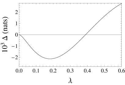
Figure 1: Difference $\Delta=\mathcal{D}(\rho_{q}^{T_{A}}|\left\{\Pi_{\vec{n}},\Pi_{0}\right\})-\mathcal{D}(\rho_{q}^{T_{A}}|\left\{\Pi_{m}\right\})$ versus the parameter $\lambda$ for the state (IV). $\mathcal{D}(\rho_{q}^{T_{A}}|\left\{\Pi_{\vec{n}},\Pi_{0}\right\})$ is the measurement-dependent discord (63) for measurement $\{\Pi_{\vec{n}},\Pi_{0}\}$ with $N=30$ and $\mathcal{D}(\rho_{q}^{T_{A}}|\left\{\Pi_{m}\right\})=\lambda\ln 2$ is the measurement-dependent discord for photon counting Tatham_12 . In the interval $0<\lambda\leq\lambda_{\rm th}\doteq 0.389$ the difference $\Delta$ is negative and the measurement $\left\{\Pi_{\vec{n}},\Pi_{0}\right\}$ outperforms photon counting. All infinite sums encountered in the expressions of entropies have been approximated by $500$-th partial sum.

V Conclusions

We have shown that all PPT CV Werner states are separable. Inspired by a method in Kraus_00 designed for $2\times N$ systems we have first decomposed all PPT truncated $N\times N$ CV Werner states into a convex mixture of product states, thus proving their separability. Next we have shown that the truncated states approximate, in the trace norm, their infinite-dimensional counterparts, which implies separability of all PPT CV Werner states. Finally, we have constructed a generalized non-Gaussian measurement from the product states of a CV Werner state decomposition and shown that the measurement extracts more non-classical correlations than photon counting, as quantified by quantum discord.

The results presented in this paper reveal a similarity between CV Werner states and the original Werner states since the PPT condition is equivalent to separability for both Horodecki_01 . This fact may also raise the question of whether Werner states share a similarity also for distillability. In particular, one may ask whether, like in the finite-dimensional case, there are NPT CV Werner states satisfying the reduction separability criterion Horodecki_99 , which would be the candidates for currently hypothetical NPT non-distillable entangled states Horodecki_09 . The answer to this question is left for future research. Besides, as the PPT CV Werner states considered here are also elements of a larger set of PPT states Chruscinski_06 possessing a similar structure, the present approach can serve as a recipe on how to analyse separability of other states from this set. We hope that our results will inspire further studies on separability and non-classical correlations in PPT quantum states both in finite- and infinite-dimensional Hilbert state spaces.

VI Acknowledgment

D. M. acknowledges the support of the Operational Program Education for Competitiveness Project No. CZ.1.07/2.3.00/20.0060 co-financed by the European Social Fund and Czech Ministry of Education. L. M. would like to acknowledge the Project No. P205/12/0694 of GAČR.

References

- (1) R. F. Werner, Phys. Rev. A 40, 4277 (1989).
- (2) N. Gisin, Phys. Lett. A 210, 151 (1996).
- (3) A. Peres, Phys. Rev. A 54, 2685 (1996).
- (4) A. Peres, Phys. Rev. Lett. 77, 1413 (1996).
- (5) M. A. Nielsen and J. Kempe, Phys. Rev. Lett. 89, 5184 (2001).
- (6) C. H. Bennett, G. Brassard, S. Popescu, B. Schumacher, J. A. Smolin, and W. K. Wootters, Phys. Rev. Lett. 76, 722 (1996).
- (7) H. Ollivier and W. H. Zurek, Phys. Rev. Lett. 02, 017901 (2002).
- (8) C. Weedbrook, S. Pirandola, J. Thompson, V. Vedral, and M. Gu, e-print arXiv:1312.3332.
- (9) L. Mišta, Jr., R. Filip, and J. Fiurášek, Phys. Rev. A 65, 062315 (2002).
- (10) R. Tatham, L. Mišta, Jr., G. Adesso, and N. Korolkova, Phys. Rev. A 85, 022326 (2012).
- (11) C. V. S. Borges, A. Z. Khoury, S. Walborn, P. H. S. Ribeiro, P. Milman, and A. Keller, Phys. Rev. A 86, 052107 (2012).
- (12) A. P. Lund, T. C. Ralph, and P. van Loock, J. Mod. Opt. 55, 2083 (2008).
- (13) C. Rodó, G. Adesso, and A. Sanpera, Phys. Rev. Lett. 100, 110505 (2008).
- (14) P. Horodecki, Phys. Lett. A 232, 333 (1997).
- (15) B. Kraus, J. I. Cirac, S. Karnas, and M. Lewenstein, Phys. Rev. A 61, 062302 (2000).
- (16) R. Clifton and H. Halvorson, Phys. Rev. A 61, 012108 (1999).
- (17) J. Eisert, C. Simon, and M. B. Plenio, J. Phys. A 35, 3911 (2002).
- (18) M. Reed and B. Simon, Methods in Modern Mathematical Physics (Academic Press, New York, 1972), Vol. 1.
- (19) G. Vidal and R. F. Werner, Phys. Rev. A 65, 032314 (2002).
- (20) A. S. Kholevo, M. E. Shirokov, and R. F. Werner, Russ. Math. Surv. 60, 359 (2005); arXiv:quant-ph/0504204.
- (21) D. Cavalcanti, L. Aolita, S. Boixo, K. Modi, M. Piani, and A. Winter, Phys. Rev. A 83, 032324 (2011).
- (22) V. Madhok and A. Datta, Phys. Rev. A 83, 032323 (2011).
- (23) M. Gu, H. M. Chrzanowski, S. M. Assad, T. Symul, K. Modi, T. C. Ralph, V. Vedral, and P. K. Lam, Nat. Phys. 8, 671 (2012).
- (24) M. P. Almeida, M. Gu, A. Fedrizzi, M. A. Broome, T. C. Ralph, and A. G. White, e-print arXiv:1301.7110.
- (25) K. Modi, A. Brodutch, H. Cable, T. Paterek, and V. Vedral, Rev. Mod. Phys. 84, 1655 (2012).
- (26) S. Luo, Phys. Rev. A 77, 022301 (2008).
- (27) D. Girolami, M. Paternostro, and G. Adesso, J. Phys. A 44, 352002 (2011).
- (28) D. T. Pegg, L. S. Phillips, and S. M. Barnett, Phys. Rev. Lett. 81, 1604 (1998).
- (29) C. J. Villas-Boas, Y. Guimarães, M. H. Y. Moussa, and B. Baseia, Phys. Rev. A 63, 055801 (2001).
- (30) J. Fiurášek, R. García-Patrón, and N. J. Cerf, Phys. Rev. A 72, 033822 (2005).
- (31) P. Horodecki and R. Horodecki, Quantum Inf. and Comp. 1, 45 (2001).
- (32) M. Horodecki and P. Horodecki, Phys. Rev. A 59, 4206 (1999).
- (33) R. Horodecki, P. Horodecki, M. Horodecki, and K. Horodecki, Rev. Mod. Phys. 81, 865 (2009).
- (34) D. Chruściński and A. Kossakowski, Phys. Rev. A 74, 022308 (2006).