A Significance Test for Covariates
in Nonparametric Regression

Abstract

We consider testing the significance of a subset of covariates in a nonparametric regression. These covariates can be continuous and/or discrete. We propose a new kernel-based test that smoothes only over the covariates appearing under the null hypothesis, so that the curse of dimensionality is mitigated. The test statistic is asymptotically pivotal and the rate of which the test detects local alternatives depends only on the dimension of the covariates under the null hypothesis. We show the validity of wild bootstrap for the test. In small samples, our test is competitive compared to existing procedures.

1 Introduction

Testing the significance of covariates is common in applied regression analysis. Sound parametric inference hinges on the correct functional specification of the regression function, but the likelihood of misspecification in a parametric framework cannot be ignored, especially as applied researchers tend to choose functional forms on the basis of parsimony and tractability. Significance testing in a nonparametric framework has therefore obvious appeal as it requires much less restrictive assumptions. Fan (1996), Fan and Li (1996) , Racine (1997), Chen and Fan (1999), Lavergne and Vuong (2000), Ait-Sahalia et al. (2001), and Delgado and González Manteiga (2001) proposed tests of significance for continuous variables in nonparametric regression models. Delgado (1993), Dette and Neumeyer (2001), Lavergne (2001), Neumeyer and Dette (2003), Racine et al. (2006) focused on significance of discrete variables. Volgushev et al. (2013) considered significance testing in nonparametric quantile regression. For each test, one needs first to estimate the model without the covariates under test, that is under the null hypothesis. The result is then used to check the significance of extra covariates. Two competing approaches are then possible. In the “smoothing approach,” one regresses the residuals onto the whole set of covariates nonparametrically, while in the “empirical process approach” one uses the empirical process of residuals marked by a function of all covariates.

In this work, we adopt an hybrid approach to develop a new significance test of a subset of covariates in a nonparametric regression. Our new test has three specific features. First, it does not require smoothing with respect to the covariates under test as in the “empirical process approach.” This allows to mitigate the curse of dimensionality that appears with nonparametric smoothing, hence improving the power properties of the test. Our simulation results show that indeed our test is more powerful than competitors under a wide spectrum of alternatives. Second, the test statistic is asymptotically pivotal as in the “smoothing approach,” while wild bootstrap can be used to obtain small samples critical values of the test. This yields a test whose level is well controlled by bootstrapping, as shown in simulations. Third, our test equally applies whether the covariates under test are continuous or discrete, showing that there is no need of a specific tailored procedure for each situation.

The paper is organized as follows. In Section 2, we present our testing procedure. In Section 3, we study its asymptotic properties under a sequence of local alternatives and we establish the validity of wild bootstrap. In Section 4, we compare the small sample behavior of our test to some existing procedures. Section 5 gathers our proofs.

2 Testing Framework and Procedure

2.1 Testing Principle

We want to assess the significance of $X\in\mathbb{R}^{q}$ in the nonparametric regression of $Y\in\mathbb{R}$ on $W\in\mathbb{R}^{p}$ and $X$. Formally, this corresponds to the null hypothesis

$$H_{0}\,:\,\mathbb{E}\left[Y\mid W,X\right]=\mathbb{E}\left[Y\mid W\right]\quad\mbox{a.s.}$$

which is equivalent to

$$H_{0}\,:\,\mathbb{E}\left[u\mid W,X\right]=0\quad\mbox{a.s.}$$ (1)

where $u=Y-\mathbb{E}\left[Y\mid W\right]$. The corresponding alternative hypothesis is

$$H_{1}\,:\,\mathbb{P}\left\{\mathbb{E}\left[u\mid W,X\right]=0\right\}<1.$$

The following result is the cornerstone of our approach. It characterizes the null hypothesis $H_{0}$ using a suitable unconditional moment equation.

Lemma 1.

Let $\left(W_{1},\,X_{1},\,u_{1}\right)$ and $\left(W_{2},\,X_{2},\,u_{2}\right)$ be two independent draws of $\left(W,\,X,\,u\right)$, $\nu(W)$ a strictly positive function on the support of $W$ such that $\mathbb{E}[u^{2}\nu^{2}(W)]<\infty$, and $K(\cdot)$ and $\psi(\cdot)$ even functions with (almost everywhere) positive Fourier integrable transforms. Define

$$I\left(h\right)=\mathbb{E}\left[u_{1}u_{2}\nu\left(W_{1}\right)\nu\left(W_{2}\right)h^{-p}K\left(\left(W_{1}-W_{2}\right)/h\right)\psi\left(X_{1}-X_{2}\right)\right]\,.$$

Then for any $h>0$,

$$\mathbb{E}\left[u\mid W,X\right]=0\,\;a.s.\Leftrightarrow I(h)=0.$$

Proof.

Let $\langle\cdot,\cdot\rangle$ denote the standard inner product. Using Fourier Inversion Theorem, change of variables, and elementary properties of conditional expectation,

$$I\left(h\right)$$

$$= \mathbb{E}\left[u_{1}u_{2}\nu\left(W_{1}\right)\nu\left(W_{2}\right)\int_{\mathbb{R}^{p}}e^{2\pi i\langle t,\;W_{1}-W_{2}\rangle}\mathcal{F}\left[K\right]\left(th\right)dt\right.$$

$$\times\left.\int_{\mathbb{R}^{q}}e^{2\pi i\langle s,\;X_{1}-X_{2}\rangle}\mathcal{F}\left[\psi\right]\left(s\right)ds\right]$$

$$= \int_{\mathbb{R}^{q}}\int_{\mathbb{R}^{p}}\left|\mathbb{E}\left[\mathbb{E}\left[u\mid W,X\right]\nu\left(W\right)e^{2\pi i\left\{\langle t,W\rangle+\langle s,X\rangle\right\}}\right]\right|^{2}\mathcal{F}\left[K\right]\left(th\right)\mathcal{F}\left[\psi\right]\left(s\right)dtds\,.$$

Since the Fourier transforms $\mathcal{F}\left[K\right]$ and $\mathcal{F}\left[\psi\right]$ are strictly positive, $I(h)=0$ iff

$$\mathbb{E}\left[\mathbb{E}\left[u\mid W,X\right]\nu\left(W\right)e^{2\pi i\left\{\langle t,W\rangle+\langle s,X\rangle\right\}}\right]=0\qquad\forall t,s\,.$$

But this is equivalent to $\mathbb{E}\left[u\mid W,X\right]\nu\left(W\right)=0$ a.s., which by our assumption on $\nu(\cdot)$ is equivalent to $H_{0}$. ∎

2.2 The Test

Lemma 1 holds whether the covariates $W$ and $X$ are continuous or discrete. For now, we assume $W$ is continuously distributed, and we later comment on how to modify our procedure in the case where some of its components are discrete. We however do not restrict $X$ to be continuous. Since it is sufficient to test whether $I(h)=0$ for any arbitrary $h$, we can choose $h$ to obtain desirable properties. So we consider a sequence of $h$ decreasing to zero when the sample size increases, which is one of the ingredient that allows to obtain a tractable asymptotic distribution for the test statistic.

Assume we have at hand a random sample $(Y_{i},W_{i},X_{i})$, $1\leq i\leq n$, from $(Y,W,X)$. In what follows, $f(\cdot)$ denotes the density of $W$, $r(\cdot)=\mathbb{E}\left[Y\mid W=\cdot\right]$, $u=Y-r(W)$, and $f_{i}$, $r_{i}$, $u_{i}$ respectively denote $f\left(W_{i}\right)$, $r\left(W_{i}\right)$, and $Y_{i}-r\left(W_{i}\right)$. Since nonparametric estimation should be entertained to approximate $u_{i}$, we consider usual kernel estimators based on kernel $L(\cdot)$ and bandwidth $g$. With $L_{nik}=\frac{1}{g^{p}}L\left(\frac{W_{i}-W_{k}}{g}\right)$, let

$$\hat{f}_{i} = (n-1)^{-1}\sum_{k\neq i,k=1}^{n}L_{nik}\,,$$

$$\hat{r}_{i} = \frac{1}{\hat{f}_{i}}\frac{1}{(n-1)}\sum_{k\neq i,k=1}^{n}Y_{k}L_{nik}\,$$

$$\mbox{so that }\quad\hat{u}_{i} = Y_{i}-\hat{r}_{i}=\frac{1}{\hat{f}_{i}}\frac{1}{(n-1)}\sum_{k\neq i,k=1}^{n}(Y_{i}-Y_{k})L_{nik}\,.$$

Denote by $n^{\left(m\right)}$ the number of arrangements of $m$ distinct elements among $n$, and by $[1/n^{\left(m\right)}]\sum_{a}$, the average over these arrangements. In order to avoid random denominators, we choose $\nu\left(W\right)=f\left(W\right)$, which fulfills the assumption of Lemma 1. Then we can estimate $I\left(h\right)$ by the second-order U-statistic

$$\widehat{I}_{n} = \frac{1}{n^{\left(2\right)}}\sum_{a}\hat{u}_{i}\hat{f}_{i}\hat{u}_{j}\hat{f}_{j}K_{nij}\psi_{ij}$$

$$= \frac{1}{n^{\left(2\right)}\left(n-1\right)^{2}}\sum_{a}\sum_{k\neq i}\sum_{l\neq j}\left(Y_{i}-Y_{k}\right)\left(Y_{j}-Y_{l}\right)L_{nik}L_{njl}K_{nij}\psi_{ij}\,,$$

with $K_{nij}=\frac{1}{h^{p}}K\left(\frac{W_{i}-W_{j}}{h}\right)$ and $\psi_{ij}=\psi\left(X_{i}-X_{j}\right)$. We also consider the alternative statistic

$$\tilde{I}_{n}=\frac{1}{n^{\left(4\right)}}\sum_{a}\left(Y_{i}-Y_{k}\right)\left(Y_{j}-Y_{l}\right)L_{nik}L_{njl}K_{nij}\psi_{ij}\,.$$

It is clear that $\tilde{I}_{n}$ is obtained from $\widehat{I}_{n}$ by removing asymptotically negligible “diagonal” terms. Under the null hypothesis, both statistics will have the same asymptotic normal distribution, but removing diagonal terms reduces the bias of the statistic under $H_{0}$. Our statistics $\tilde{I}_{n}$ and $\widehat{I}_{n}$ are respectively similar to the ones of Fan and Li (1996) and Lavergne and Vuong (2000), with the fundamental difference that there is no smoothing relative to the covariates $X$. Indeed these authors used a multidimensional smoothing kernel over $(W,X)$, that is $h^{-\left(p+q\right)}\tilde{K}\left(\left(W_{i}-W_{j}\right)/h,\,\left(X_{i}-X_{j}\right)/h\right)$, while we use $K_{nij}\psi_{ij}$. For $I_{n}$ being either $\tilde{I}_{n}$ or $\widehat{I}_{n}$, we will show that $nh^{p/2}I_{n}\mbox{$\stackrel{{\scriptstyle d}}{{\longrightarrow}}\,$}\mathcal{N}\left(0,\omega^{2}\right)$ under $H_{0}$ and $nh^{p/2}I_{n}\mbox{$\stackrel{{\scriptstyle p}}{{\longrightarrow}}\,$}\infty$ under $H_{1}$. By contrast, the statistics of Fan and Li (1996) and Lavergne and Vuong (2000) exhibit a $nh^{(p+q)/2}$ rate of convergence. The alternative test of Delgado and González Manteiga (2001) uses the kernel residuals $\hat{u}_{i}$ and the empirical process approach of Stute (1997). This avoids extra smoothing, but a the cost of a test statistic with a non pivotal asymptotic law under $H_{0}$. Hence, our proposal is an hybrid approach that combines the advantages of existing procedures, namely smoothing only for the variables $W$ appearing under the null hypothesis but with an asymptotic normal distribution for the statistic. Given a consistent estimator $\omega^{2}_{n}$ of $\omega^{2}$, as provided in the next section, we obtain an asymptotic $\alpha$-level test of $H_{0}$ as

$$\mbox{Reject }H_{0}\mbox{ if }\ nh^{p/2}I_{n}/\omega_{n}>z_{1-\alpha}\,,$$

where $z_{1-\alpha}$ is the $(1-\alpha)$-th quantile of the standard normal distribution. In small samples, we will show the validity of a wild bootstrap scheme to obtain critical values.

The test applies whether $X$ is continuous or has some discrete components. The procedure is also easily adapted to some discrete components of $W$. In that case, one would replace kernel smoothing by cells’ indicators for the discrete components, so that for $W$ composed of continuous $W_{c}$ of dimension $p_{c}$ and discrete $W_{d}$, one would use $h^{-p_{c}}K\left(\frac{W_{ic}-W_{jc}}{h}\right)\mathbb{I}(W_{id}=W_{jd})$ instead of $K_{nij}$. It would also be possible to smooth on the discrete components, as proposed by Racine and Li (2004). To obtain scale invariance, we recommend that observations on covariates should be scaled, say by their sample standard deviation as is customary in nonparametric estimation. It is equally important to scale the $X_{i}$ before they are used as arguments of $\psi(\cdot)$ to preserve such invariance.

The outcome of the test may depend on the choice of the kernels $K(\cdot)$ and $L(\cdot)$, while this influence is expected to be limited as it is in nonparametric estimation. The choice of the function $\psi(\cdot)$ might be more important, but our simulations reveal that it is not. From our theoretical study, this function, as well as $K(\cdot)$ should possess an almost everywhere positive and integrable Fourier transform. This is true for (products of) the triangular, normal, Laplace, and logistic densities, see Johnson et al. (1995), and for a Student density, see Hurst (1995). Alternatively, one can choose $\psi(x)$ as a univariate density applied to some transformation of $x$, such as its norm. This yields $\psi(x)=g\left(\|x\|\right)$ where $g(\cdot)$ is any of the above univariate densities. This is the form we will consider in our simulations to study the influence of $\psi(\cdot)$.

3 Theoretical Properties

We here give the asymptotic properties of our test statistics under $H_{0}$ and some local alternatives. To do so in a compact way, we consider the sequence of hypotheses

$$H_{1n}\,:\,\mathbb{E}\left[Y\mid W,X\right]=r\left(W\right)+\delta_{n}d\left(W,X\right),\qquad n\geq 1,$$

where $d(\cdot)$ is a fixed integrable function. Since $r\left(W\right)=\mathbb{E}\left[Y\mid W\right]$, our setup imposes $\mathbb{E}\left[d\left(W,X\right)\mid W\right]=0$. The null hypothesis corresponds to the case $\delta_{n}\equiv 0$, while considering a sequence $\delta_{n}\to 0$ yields local Pitman-like alternatives.

3.1 Assumptions

We begin by some useful definitions.

Definition 1.

(i)

$\mathcal{U}^{p}$ is the class of integrable uniformly continuous functions from $\mathbb{R}^{p}$ to $\mathbb{R}$;

(ii)

$\mathcal{D}_{s}^{p}$ is the class of $m$-times differentiable functions from $\mathbb{R}^{p}$ to $\mathbb{R}$ , with derivatives of order $\left\lfloor s\right\rfloor$ that are uniformly Lipschitz continuous of order $s-\left\lfloor s\right\rfloor$, where $\left\lfloor s\right\rfloor$ denotes the integer such that $\left\lfloor s\right\rfloor\leq s<\left\lfloor s\right\rfloor+1$.

Note that a function belonging to $\mathcal{U}^{p}$ is necessarily bounded.

Definition 2.

$\mathcal{K}_{m}^{p}$, $m\geq 2$, is the class of even integrable functions $K\,:\,\mathbb{R}^{p}\to\mathbb{R}$ with compact support satisfying $\int K\left(t\right)dt=1$ and, if $t=(t_{1},\dots,t_{p})$,

$$\int_{\mathbb{R}^{p}}t_{1}^{\alpha_{1}}\dots t_{p}^{\alpha_{p}}K\left(t\right)dt=0\;\;\mbox{ for }\;\;0<\sum_{i=1}^{p}\alpha_{i}\leq m-1,\,\alpha_{i}\in\mathbb{N}\quad\forall i$$

This definition of higher-order kernels is standard in nonparametric estimation. The compact support assumption is made for simplicity and could be relaxed at the expense of technical conditions on the rate of decrease of the kernels at infinity, see e.g. Definition 1 in Fan and Li (1996). In particular, the gaussian kernel could be allowed for. We are now ready to list our assumptions.

Assumption 1.

(i) For any $x\in\mathbb{R}^{q}$ in the support of $X$, the vector $W$ admits a conditional density given $X=x$ with respect to the Lebesgue measure in $\mathbb{R}^{p}$, denoted by $\pi(\cdot\mid x)$. Moreover, $\mathbb{E}\left[Y^{8}\right]<\infty$. (ii) The observations $\left(W_{i},X_{i},Y_{i}\right)$, $i=1,\cdots,n$ are independent and identically distributed as $(W,X,Y)$.

The existence of the conditional density given $X=x$ for all $x\in\mathbb{R}^{q}$ in the support of $X$ implies that $W$ admits a density with respect to the Lebesgue measure on $\mathbb{R}^{p}$. As noted above, our results easily generalizes to some discrete components of $W$, but for the sake of simplicity we do not formally consider this in our theoretical analysis.

Assumption 2.

(i)

$f\left(\cdot\right)$ and $r\left(\cdot\right)f\left(\cdot\right)$ belong to $\mathcal{U}^{p}\cap\mathcal{D}_{s}^{p}$, $s\geq 2$;

(ii)

$\mathbb{E}\left[u^{2}\mid W=\cdot\right]f\left(\cdot\right)$, $\mathbb{E}\left[u^{4}\mid W=\cdot\right]f^{4}\left(\cdot\right)$ belong to $\mathcal{U}^{p};$

(iii)

the function $\psi\left(\cdot\right)$ is bounded and has a almost everywhere positive and integrable Fourier transform;

(iv)

$K\left(\cdot\right)\in\mathcal{K}_{2}^{p}$ and has an almost everywhere positive and integrable Fourier transform, while $L\left(\cdot\right)\in\mathcal{K}_{\left\lfloor s\right\rfloor}^{p}$ and is of bounded variation;

(v)

let $\sigma^{2}(w,x)=\mathbb{E}[u^{2}\mid W=w,X=x]$, then $\sigma^{2}\left(\cdot,x\right)f^{2}\left(\cdot\right)\pi\left(\cdot\mid x\right)$ belongs to $\mathcal{U}^{p}$ for any $x$ in the support of $X$, has integrable Fourier transform, and

$\mathbb{E}\left[\sigma^{4}\left(W,X\right)f^{4}\left(W\right)\pi\left(W\mid X\right)\right]<\infty$;

(vi)

$\mathbb{E}[d^{2}(W,X)\mid W=\cdot]f^{2}(\cdot)$ belongs to $\mathcal{U}^{p}$, $d(\cdot,x)f\left(\cdot\right)\pi\left(\cdot\mid x\right)$ is integrable and squared integrable for any $x$ in the support of $X$, and

$\mathbb{E}\left[d^{2}\left(W,X\right)f^{2}\left(W\right)\pi\left(W\mid X\right)\right]<\infty$.

Standard regularity conditions are assumed for various functions. A higher-order kernel $L(\cdot)$ is used in conjunction with the differentiability conditions in (i) to ensure that the bias in nonparametric estimation is small enough.

3.2 Asymptotic Analysis

The following result characterizes the behavior of our statistics under the null hypothesis and a sequence of local alternatives.

Theorem 1.

Let $I_{n}$ be any of the statistics $\widehat{I}_{n}$ or $\tilde{I}_{n}$. Under Assumptions 1 and 2, and if as $n\to\infty$ (i) $g,h\to 0$, (ii) $n^{7/8}g^{p}/\ln n,$ $nh^{p}\to\infty$, (iii) $nh^{p/2}g^{2s}\to 0$, and (iv) $h/g\to 0$ if $I_{n}=\tilde{I}_{n}$ or $h/g^{2}\to 0$ if $I_{n}=\widehat{I}_{n}$, then

(i)

If $\delta_{n}^{2}nh^{p/2}\to C$ with $0\leq C<\infty$, $nh^{p/2}I_{n}\mbox{$\stackrel{{\scriptstyle d}}{{\longrightarrow}}\,$}\mathcal{N}\left(C\mu,\omega^{2}\right)$ where

$$\mu=\mathbb{E}\left[\intop\!\!d\left(w,X_{1}\right)d\left(w,X_{2}\right)f^{2}\left(w\right)\pi\left(w\mid X_{1}\right)\pi\left(w\mid X_{2}\right)\psi\left(X_{1}\!-\!X_{2}\right)dw\right]>0$$

$$\mbox{and }\quad\omega^{2}=2\int\!K^{2}\!\left(s\right)\,ds$$

$$\mathbb{E}\left[\int\!\!\sigma^{2}\left(w,X_{1}\right)\sigma^{2}\left(w,X_{2}\right)f^{4}\left(w\right)\pi\left(w\mid X_{1}\right)\pi\left(w\mid X_{2}\right)\psi^{2}\left(X_{1}\!-\!X_{2}\right)dw\right]\,.$$

(ii)

If $\delta_{n}^{2}nh^{p/2}\to\infty$, $nh^{p/2}I_{n}\mbox{$\stackrel{{\scriptstyle p}}{{\longrightarrow}}\,$}\infty$.

The rate of convergence of the test statistic depends only on the dimension of $W$, the covariates present under the null hypothesis, but not on the dimension of $X$, the covariates under test. Similarly, the rate of local alternatives that are detected by the test depends only on the dimension of $W$. As shown in the simulations, this yields some gain in power compared to competing “smoothing” tests. Conditions (i) to (iv) together require that $s>p/2$ for $I_{n}=\tilde{I}_{n}$ and $s>p/4$ for $I_{n}=\widehat{I}_{n}$, so removing diagonal terms in $\widehat{I}_{n}$ allows to weaken the restrictions on the bandwidths. Condition (ii) could be slightly weakened to $ng^{p}\rightarrow\infty$ at the price of handling high order $U$-statistics in the proofs, but allows for a shorter argument based on empirical processes, see Lemma 3 in the proofs section.

To estimate $\omega^{2}$, we can either mimic Lavergne and Vuong (2000) to consider

$$\tilde{\omega}_{n}^{2}=\dfrac{2h^{p}}{n^{\left(6\right)}}\sum_{a}\left(Y_{i}-Y_{k}\right)\left(Y_{i}-Y_{k^{\prime}}\right)\left(Y_{j}-Y_{l}\right)\left(Y_{j}-Y_{l^{\prime}}\right)L_{nik}L_{nik^{\prime}}L_{njl}L_{njl^{\prime}}K_{nij}^{2}\psi_{ij}^{2},$$

or generalize the variance estimator of Fan and Li (1996) as

$$\widehat{\omega}_{n}^{2}=\dfrac{2h^{p}}{n^{\left(2\right)}}\sum_{a}\hat{u}_{i}^{2}\hat{f}_{i}^{2}\hat{u}_{j}^{2}\hat{f}_{j}^{2}K_{nij}^{2}\psi_{ij}^{2}.$$

The first one is consistent for $\omega^{2}$ under both the null and alternative hypothesis, but the latter is faster to compute.

Corollary 1.

Let $I_{n}$ be any of the statistics $\widehat{I}_{n}$ or $\tilde{I}_{n}$ and let $\omega_{n}$ denote any of $\widehat{\omega}_{n}$ or $\tilde{\omega}_{n}$. Under the assumptions of Theorem 1, the test that rejects $H_{0}$ when $nh^{p/2}I_{n}/\omega_{n}>z_{1-\alpha}$ is of asymptotic level $\alpha$ under $H_{0}$ and is consistent under the sequence of local alternatives $H_{1n}$ provided $\delta_{n}^{2}nh^{p/2}\to\infty$.

3.3 Bootstrap Critical Values

It is known that asymptotic theory may be inaccurate for small and moderate samples when using smoothing methods. Hence, as in e.g. Härdle and Mammen (1993) or Delgado and González Manteiga (2001), we consider a wild bootstrap procedure to approximate the quantiles of our test statistic. Resamples are obtained from $Y_{i}^{*}=\hat{r}_{i}+u_{i}^{*}$, where $u_{i}^{*}=\eta_{i}\hat{u}_{i}$ and $\eta_{i}$ are i.i.d. variables independent of the initial sample with $\mathbb{E}\eta_{i}=0$ and $\mathbb{E}\eta_{i}^{2}=\mathbb{E}\eta_{i}^{3}=1$, $1\leq i\leq n$. The $\eta_{i}$ could for instance follow the two-point law of Mammen (1993). With at hand a bootstrap sample $(Y_{i}^{*},W_{i},X_{i})$, $1\leq i\leq n$, we obtain a bootstrapped statistic $I_{n}^{*}$ with bootstrapped observations $Y_{i}^{*}$ in place of original observations $Y_{i}$. When the scheme is repeated many times, the bootstrap critical value $z^{\star}_{1-\alpha,n}$ at level $\alpha$ is the empirical $(1-\alpha)$-th quantile of the bootstrapped test statistics. The asymptotic validity of this bootstrap procedure is guaranteed by the following result.

Theorem 2.

Suppose Assumptions 1, 2, and Conditions (i) to (iii) of Theorem 1 hold. Moreover, assume $\inf_{w\in\mathcal{S}_{W}}f\left(w\right)>0$ and $h/g^{2}\to 0$. Then for $I_{n}^{*}$ equal to any of $\widehat{I}_{n}^{*}$ and $\tilde{I}_{n}^{*}$,

$$\sup_{z\in\mathbb{R}}\left|\mathbb{P}\left[nh^{p/2}I_{n}^{*}/\omega_{n}^{*}\leq z\mid Y_{1},W_{1},X_{1},\cdots,Y_{n},W_{n},X_{n}\right]-\Phi\left(z\right)\right|\mbox{$\stackrel{{\scriptstyle p}}{{\longrightarrow}}\,$}0\,,$$

where $\Phi\left(\cdot\right)$ is the standard normal distribution function.

4 Monte Carlo Study

We investigated the small sample behavior of our test and studied its performances relative to alternative tests. We generated data through

$$Y=\left(W^{\prime}\theta\right)^{3}-W^{\prime}\theta+\delta d\left(X\right)+\varepsilon$$

where $W$ follow a two-dimensional standard normal, $X$ independently follows a $q$-variate standard normal, $\varepsilon\sim\mathcal{N}\left(0,4\right)$, and we set $\theta=\left(1,\,-1\right)^{\prime}/\sqrt{2}$. The null hypothesis corresponds to $\delta=0$, and we considered various forms for $d(\cdot)$ to investigate power. We only considered the test based on $\tilde{I}_{n}$, labelled LMP, as preliminary simulation results showed that it had similar or better performances than the test based on $\widehat{I}_{n}$. We compared it to the test of Lavergne and Vuong (2000, hereafter LV), and the test of Delgado and Gonzalez-Manteiga (2001, hereafter DGM). The statistic for the latter test is the Cramer-von-Mises statistic

$$\sum_{i=1}^{n}\left[\sum_{j=1}^{n}{\widehat{u}_{j}}\widehat{f}_{j}\,\mathbf{1}\left\{W_{j}\leq W_{i}\right\}\,\mathbf{1}\left\{X_{j}\leq X_{i}\right\}\right]^{2}\,,$$

and critical values are obtained by wild bootstrapping as for our own statistic. To compute bootstrap critical values, we used 199 bootstrap replications and the two-point distribution

$$\mathbb{P}\left(\eta_{i}=\frac{1-\sqrt{5}}{2}\right)=\frac{5+\sqrt{5}}{10}\;,\;\mathbb{P}\left(\eta_{i}=\frac{1+\sqrt{5}}{2}\right)=\frac{5-\sqrt{5}}{10}\;.$$

For all tests, each time a kernel appears, we used the Epanechnikov kernel applied to the norm of its argument $u$, that is $0.75\,\left(1-\left\|u\right\|^{2}\right)\mathbf{1}\left\{\left\|u\right\|<1\right\}$. The bandwidth parameters are set to $g=n^{-1/6}$ and $h=c\,n^{-2.1/6}$, and we let $c$ vary to investigate the sensitivity of our results to the smoothing parameter’s choice. To study the influence of $\psi(\cdot)$ on our test, we considered $\psi(x)=l\left(\left\|x\right\|\right)$, where $l(\cdot)$ is a triangular or normal density, each with a second moment equal to one.

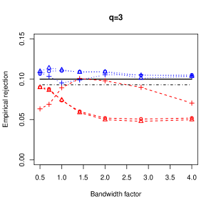
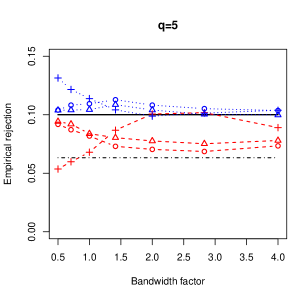
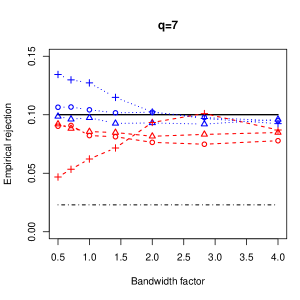
Figure 1: Empirical rejections under $H_{0}$ as a function of the bandwidth, $n=100$

Figure 1 reports the empirical level of the various tests for $n=100$ based on 5000 replications when we let $c$ and $q$ vary. For our test, bootstrapping yields more accurate rejection levels than the asymptotic normal critical values for any bandwidth factor $c$ and dimension $q$. The choice of $\psi(\cdot)$ does not influence the results. The empirical level of LV test is much more sensitive to the bandwidth and the dimension. The empirical level of the DGM test is close to the nominal one for a low dimension $q$, but decreases with increasing $q$.

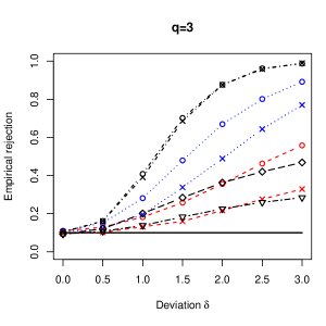
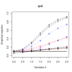
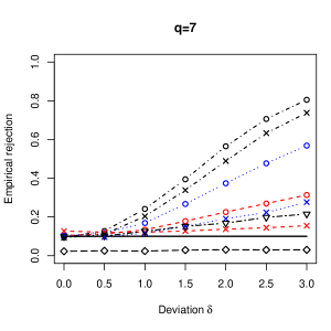
Figure 2: Empirical power curves for a quadratic alternative, $n=100$

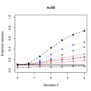
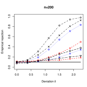
Figure 3: Empirical power curves for a quadratic alternative, $q=5$

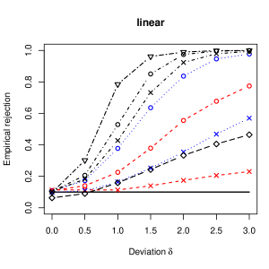
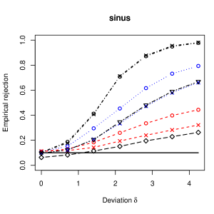
Figure 4: Empirical power curves for linear and sine alternative, $n=100$ and $q=5$

To investigate power, we considered different forms of alternatives as specified by $d(\cdot)$. We first focus on a quadratic alternative, where $d\left(X\right)=\left(X^{\prime}\beta-1\right)^{2}/\sqrt{2}$, with $\beta=\left(1,\,,1,\,,\dots\right)^{\prime}/\sqrt{q}$. Figure 2 reports power curves of the different tests for the quadratic alternative, $n=100$, and a nominal level of 10% based on $2000$ replications. We also report the power of a Fisher test based on a linear specification in the components of $X$. The power of our test, as well as the one of LV test, increases when the bandwidth factor $c$ increases. This is in line with theoretical findings, though we may expect this relationship to revert for very large bandwidths. Our test always dominates LV test, as well as the Fisher test and DGM test, for any choice of $c$ and any dimension $q$. The power of all tests decreases when the dimension $q$ increases, but the more notable degradation is for the DGM test. In Figure 3, we let $n$ vary for a fixed dimension $q=5$. The power of all tests improve, but our main qualitative findings are not affected. It is noteworthy that the power advantage of our test compared to LV test become more pronounced as $n$ increases. In Figure 4, we considered a linear alternative $d\left(X\right)=X^{\prime}\beta$ and a sine alternative, $d\left(X\right)=\sin\left(2\,X^{\prime}\beta\right)$. Our main findings remain unchanged. For a linear alternative, the Fisher test is most powerful as expected. Compared to this benchmark, the loss of power when using our test is moderate for a large enough bandwidth factors $c$. For a sine alternative, our test is more powerful than the Fisher test for $c=2$ or 4.

We also considered the case of a discrete $X$. We generated data following

$$Y=\left(W^{\prime}\theta\right)^{3}-W^{\prime}\theta+\delta d\left(W\right)\,\mathbf{1}\left\{X=1\right\}+\varepsilon$$

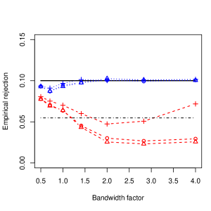
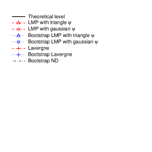
Figure 5: Empirical rejection under $H_{0}$ as a function of the bandwidth, $X$ Bernoulli and $n=100$

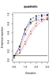
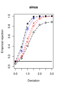
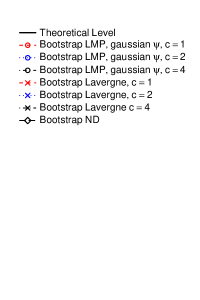
Figure 6: Empirical power curves, $X$ Bernoulli and $n=100$

where $W$ and $\varepsilon$ are generated as before, and $X$ is Bernoulli with probability of success $p=0.6$. We compared our test to two competitors. The test proposed by Lavergne (2001) is similar to our test with the main difference that $\psi(\cdot)$ is the indicator function, i.e. $\psi\left(X_{i}-X_{j}\right)=\mathbf{1}\left\{X_{i}=X_{j}\right\}$. The test of Neumeyer et Dette (2003, hereafter ND) is similar in spirit to the DGM test. The details of the simulations are similar to above. Figures 5 and 6 report our results. Bootstrapping our test and Lavergne’s test yield accurate rejection levels, while the asymptotic tests and the ND test underrejects. Under a quadratic alternative, the power of our test is comparable to the one of the ND test for a large enough bandwidth factor $c$. Under a sine alternative, our test outperforms ND test in all cases.

5 Conclusion

We have developed a testing procedure for the significance of covariates in a nonparametric regression. Smoothing is entertained only for the covariates under the null hypothesis. The resulting test statistic is asymptotically pivotal, and wild bootstrap can be used to obtain critical values in small and moderate samples. The test is versatile, as it applies whether the covariates under test are continuous and/or discrete. Simulations reveal that our test outperforms its competitors in many situations, and especially when the dimension of covariates is large.

6 Proofs

We here provide the proofs of the main results. Technical lemmas are relegated to the Appendix.

In the following, for any integrable function $\delta(X),$ let $\mathcal{F}_{X}\left[\delta\right]\left(u\right)=\mathbb{E}[e^{-2\pi i\langle X,\;u\rangle}\delta\left(X\right)],$ $u\in\mathbb{R}^{q}.$ Moreover, for any index set $I$ not containing $i$ with cardinality $\left|I\right|$, define

$$\widehat{f_{i}^{I}}=\left(n-\left|I\right|-1\right)^{-1}\sum_{k\neq i,k\notin I}L_{nik},$$

consistent with $\widehat{f_{i}}$ that corresponds to the case where $I$ is the empty set.

6.1 Proof of Theorem 1

We first consider the case $I_{n}=\tilde{I}_{n}$. Next, we study the difference between $\tilde{I}_{n}$ and $\widehat{I}_{n}$ and hence deduce the result for $I_{n}=\widehat{I}_{n}$.

Case $I_{n}=\tilde{I}_{n}$.

Consider the decomposition

$$I_{n} = \frac{1}{n^{\left(4\right)}}\sum_{a}\left(u_{i}-u_{k}\right)\left(u_{j}-u_{l}\right)L_{nik}L_{njl}K_{nij}\psi_{ij}$$

$$+\frac{2}{n^{\left(4\right)}}\sum_{a}\left(u_{i}-u_{k}\right)\left(r_{j}-r_{l}\right)L_{nik}L_{njl}K_{nij}\psi_{ij}$$

$$+\frac{1}{n^{\left(4\right)}}\sum_{a}\left(r_{i}-r_{k}\right)\left(r_{j}-r_{l}\right)L_{nik}L_{njl}K_{nij}\psi_{ij}$$

$$= I_{1}+2I_{2}+I_{3},$$

where

$$I_{1} = \frac{n-2}{n-3}\frac{1}{n^{(2)}}\sum_{a}u_{i}u_{j}f_{i}f_{j}K_{nij}\psi_{ij}+\frac{2\left(n-2\right)}{n-3}\frac{1}{n^{\left(2\right)}}\sum_{a}u_{i}\left(\widehat{f}_{i}^{j}-f_{i}\right)u_{j}f_{j}K_{nij}\psi_{ij}$$

$$+\frac{n-2}{n-3}\frac{1}{n^{(2)}}\sum_{a}u_{i}\left(\widehat{f}_{i}^{j}-f_{i}\right)u_{j}\left(\widehat{f}_{j}^{i}-f_{j}\right)K_{nij}\psi_{ij}-\frac{2}{n^{(3)}}\sum_{a}u_{i}f_{i}u_{l}L_{njl}K_{nij}\psi_{ij}$$

$$-\frac{2}{n^{\left(3\right)}}\sum_{a}u_{i}\left(\widehat{f}_{i}^{j,l}-f_{i}\right)u_{l}L_{njl}K_{nij}\psi_{ij}+\frac{1}{n^{\left(4\right)}}\sum_{a}u_{k}u_{l}L_{nik}L_{njl}K_{nij}\psi_{ij}$$

$$-\frac{1}{n^{\left(4\right)}}\sum_{a}u_{i}u_{j}L_{nik}L_{njk}K_{nij}\psi_{ij}$$

$$= \frac{n-2}{n-3}\left[I_{0n}+2I_{1,1}+I_{1,2}\right]-2I_{1,3}-2I_{1,4}+I_{1,5}-I_{1,6},$$

and

$$I_{2} = \frac{1}{n^{\left(3\right)}}\sum_{a}u_{i}f_{i}\left(r_{j}-r_{l}\right)L_{njl}K_{nij}\psi_{ij}+\frac{1}{n^{\left(3\right)}}\sum_{a}u_{i}\left(\widehat{f}_{i}^{j,l}-f_{i}\right)\left(r_{j}-r_{l}\right)L_{njl}K_{nij}\psi_{ij}$$

$$-\frac{1}{n^{\left(4\right)}}\sum_{a}u_{k}\left(r_{j}-r_{l}\right)L_{nik}L_{njl}K_{nij}\psi_{ij}=I_{2,1}+I_{2,2}-I_{2,3}.$$

In Proposition 1 we prove that, under $H_{0},$ $I_{0n}$ is asymptotically centered Gaussian with variance $\omega^{2}$, while in Proposition 2 we prove that, under $H_{1n},$ $I_{0n}$ is asymptotically Gaussian with mean $\mu$ and variance $\omega^{2}$ provided $\delta_{n}^{2}nh^{p/2}$ converges to some positive real number. In Propositions 3 and 4 we show that all remaining terms in the decomposition of $I_{n}$ are asymptotically negligible.

Proposition 1.

Under the conditions of Theorem 1, $nh^{p/2}I_{0n}\mbox{$\stackrel{{\scriptstyle d}}{{\longrightarrow}}\,$}\mathcal{N}\left(0,\omega^{2}\right)$ under $H_{0}$.

Proof.

Let us define the martingale array $\left\{S_{n,m},\mathcal{F}_{n,m},\,1\leq m\leq n,\,n\geq 1\right\}$ where $S_{n,1}=0,$ and

$$S_{n,m}=\sum_{i=1}^{m}G_{n,i}\;\;\;\text{ with }\;\;\;G_{n,i}=\dfrac{2h^{p/2}}{n-1}u_{i}f_{i}\sum_{j=1}^{i-1}u_{j}f_{j}K_{nij}\psi_{ij},\qquad 2\leq i,m\leq n,$$

and $\mathcal{F}_{n,m}$ is the $\sigma-$field generated by $\left\{W_{1},\,\dots,\,W_{n},\,X_{1},\,\dots,\,X_{n},\,Y_{1},\,\dots,\,Y_{m}\right\}.$ Thus $nh^{p/2}I_{0n}=S_{n,n}$. Also define

$$V_{n}^{2}=\sum_{i=2}^{n}E\left[G_{n,i}^{2}\mid\mathcal{F}_{n,i-1}\right]=\dfrac{4h^{p}}{\left(n-1\right)^{2}}\sum_{i=2}^{n}\sigma_{i}^{2}f_{i}^{2}\left(\sum_{j=1}^{i-1}u_{j}f_{j}K_{nij}\psi_{ij}\right)^{2}$$

where $\sigma_{i}^{2}=\sigma^{2}\left(W_{i},X_{i}\right)$. We can decompose $V_{n}^{2}$ as

$$V_{n}^{2} = \dfrac{4h^{p}}{\left(n-1\right)^{2}}\sum_{i=2}^{n}\sigma_{i}^{2}f_{i}^{2}\sum_{j=1}^{i-1}\sum_{k=1}^{i-1}u_{j}f_{j}u_{k}f_{k}K_{nij}K_{nik}\psi_{ij}\psi_{ik}$$

$$= \dfrac{4h^{p}}{\left(n-1\right)^{2}}\sum_{i=2}^{n}\sum_{j=1}^{i-1}\sigma_{i}^{2}f_{i}^{2}u_{j}^{2}f_{j}^{2}K_{nij}^{2}\psi_{ij}^{2}$$

$$+\dfrac{8h^{p}}{\left(n-1\right)^{2}}\sum_{i=3}^{n}\sum_{j=2}^{i-1}\sum_{k=1}^{j-1}\sigma_{i}^{2}f_{i}^{2}u_{j}f_{j}u_{k}f_{k}K_{nij}K_{nik}\psi_{ij}\psi_{ik}=A_{n}+B_{n}.$$

The result follows from the Central Limit Theorem for martingale arrays, see Corollary 3.1 of Hall and Heyde (1980). The conditions required for Corollary 3.1 of Hall and Heyde (1980), among which $V_{n}^{2}\mbox{$\stackrel{{\scriptstyle p}}{{\longrightarrow}}\,$}\omega^{2}$, are checked in Lemma 2 below. Its proof is provided in the Appendix.

Lemma 2.

Under the conditions of Proposition 1,

1. $A_{n}\mbox{$\stackrel{{\scriptstyle p}}{{\longrightarrow}}\,$}\omega^{2}$,

2. $B_{n}\mbox{$\stackrel{{\scriptstyle p}}{{\longrightarrow}}\,$}0$,

3. the martingale difference array $\left\{G_{n,i},\,\mathcal{F}_{n,i},\,1\leq i\leq n\right\}$ satisfies the Lindeberg condition

   $$\forall\varepsilon>0,\quad\sum_{i=2}^{n}\mathbb{E}\left[G_{n,i}^{2}I\left(\left|G_{n,i}\right|>\varepsilon\right)\mid\mathcal{F}_{n,i-1}\right]\mbox{$\stackrel{{\scriptstyle p}}{{\longrightarrow}}\,$}0\,.$$

∎

Proposition 2.

Under the conditions of Theorem 1 and $H_{1n},$ if $\delta_{n}^{2}nh^{p/2}\rightarrow C$ with $0<C<\infty,$ $nh^{p/2}I_{0n}\mbox{$\stackrel{{\scriptstyle d}}{{\longrightarrow}}\,$}\mathcal{N}\left(C\mu,\omega^{2}\right)$.

Proof.

Let $\varepsilon_{i}=Y_{i}-\mathbb{E}\left[Y_{i}\mid W_{i},\,X_{i}\right]$ and let us decompose

$$nh^{p/2}I_{0n} = \dfrac{h^{p/2}}{n-1}\sum_{i=1}^{n}\sum_{j\neq i}u_{i}f_{i}u_{j}f_{j}K_{nij}\psi_{ij}$$

$$= \dfrac{h^{p/2}}{n-1}\sum_{i=1}^{n}\sum_{j\neq i}\left(\delta_{n}d_{i}+\varepsilon_{i}\right)f_{i}\left(\delta_{n}d_{j}+\varepsilon_{j}\right)f_{j}K_{nij}\psi_{ij}$$

$$= \dfrac{h^{p/2}}{n-1}\sum_{i=1}^{n}\sum_{j\neq i}\varepsilon_{i}f_{i}\varepsilon_{j}f_{j}K_{nij}\psi_{ij}+\dfrac{\delta_{n}h^{p/2}}{n-1}\sum_{i=1}^{n}\sum_{j\neq i}d_{i}f_{i}\left(\delta_{n}d_{j}+2\varepsilon_{j}\right)f_{j}K_{nij}\psi_{ij}$$

$$= C_{0n}+C_{n}.$$

By Proposition 1, $C_{0n}\mbox{$\stackrel{{\scriptstyle d}}{{\longrightarrow}}\,$}\mathcal{N}\left(0,\omega^{2}\right).$ As for $C_{n}$, we have

$$\mathbb{E}\left[C_{n}\right]=\delta_{n}^{2}nh^{p/2}\mathbb{E}\left[d_{i}f_{i}d_{j}f_{j}K_{nij}\psi_{ij}\right]=\delta_{n}^{2}nh^{p/2}\mu_{n}\,.$$

By repeated application of Fubini’s Theorem, Fourier Inverse formula, Dominated Convergence Theorem, and Parseval’s identity, we obtain

$$\mu_{n} = \mathbb{E}\left[d_{1}f_{2}d_{1}f_{2}K_{n12}\psi_{12}\right]$$

$$= \mathbb{E}\left[\iint d\left(w_{1},X_{1}\right)d\left(w_{2},X_{2}\right)f\left(w_{1}\right)f\left(w_{2}\right)f\left(w_{1}|X_{1}\right)f\left(w_{2}|X_{2}\right)\right.$$

$$\qquad\qquad\qquad\qquad\qquad\qquad\qquad\qquad\qquad\qquad\times\left.h^{-p}K\left(\dfrac{w_{1}-w_{2}}{h}\right)dw_{1}dw_{2}\;\,\psi\left(X_{1}-X_{2}\right)\right]$$

$$= \mathbb{E}\left[\int\!\!\mathcal{F}\!\left[d\left(\cdot,X_{1}\right)\!f\left(\cdot\right)\pi\left(\cdot\mid X_{1}\right)\right]\!\left(t\right)\mathcal{F}\left[d\left(\cdot,X_{2}\right)\!f\left(\cdot\right)\pi\left(\cdot\mid X_{2}\right)\right]\!\left(-t\right)\mathcal{F}\left[K\right]\left(ht\right)dt\;\psi\left(X_{1}-X_{2}\right)\right]$$

$$\to \mathbb{E}\left[\left[\int\mathcal{F}\left[d\left(\cdot,X_{1}\right)f\left(\cdot\right)\pi\left(\cdot\mid X_{1}\right)\right]\left(t\right)\mathcal{F}\left[d\left(\cdot,X_{2}\right)f\left(\cdot\right)\pi\left(\cdot\mid X_{2}\right)\right]\left(-t\right)dt\;\right]\psi\left(X_{1}-X_{2}\right)\right]$$

$$= \mathbb{E}\left[\int d\left(w,X_{1}\right)d\left(w,X_{2}\right)f^{2}\left(w\right)\pi\left(w\mid X_{1}\right)\pi\left(w\mid X_{2}\right)\psi\left(X_{1}-X_{2}\right)dw\right]$$

$$= \int\left[\int\mathcal{F}_{X}\left[d\left(w,\cdot\right)\pi\left(w\mid\cdot\right)\right](u)\mathcal{F}_{X}\left[d\left(w,\cdot\right)\pi\left(w\mid\cdot\right)\right](-u)\mathcal{F}[\psi](u)du\right]f^{2}\left(w\right)dw$$

$$= \iint\left|\mathcal{F}_{X}\left[d\left(w,\cdot\right)\pi\left(w\mid\cdot\right)\right](u)\right|^{2}\mathcal{F}[\psi](u)f^{2}\left(w\right)dudw=\mu\,.$$

Moreover,

$$\mbox{Var}\left[C_{n}\right] \leq \dfrac{4\delta_{n}^{4}h^{p}}{\left(n-1\right)^{2}}\sum_{a}\mathbb{E}\left[d_{i}^{2}f_{i}^{2}d_{k}d_{l}f_{k}f_{l}K_{nik}K_{nil}\psi_{ik}\psi_{il}\right]$$

$$+\dfrac{2\delta_{n}^{4}h^{p}}{\left(n-1\right)^{2}}\sum_{a}\mathbb{E}\left[d_{i}^{2}f_{i}^{2}d_{k}^{2}f_{k}^{2}K_{nik}^{2}\psi_{ik}^{2}\right]$$

$$+\dfrac{4\delta_{n}^{2}h^{p}}{\left(n-1\right)^{2}}\sum_{a}\mathbb{E}\left[d_{i}f_{i}d_{j}f_{j}\varepsilon_{k}^{2}f_{k}^{2}K_{nik}K_{njk}\psi_{ik}\psi_{jk}\right]$$

$$+\dfrac{4\delta_{n}^{2}h^{p}}{\left(n-1\right)^{2}}\sum_{a}\mathbb{E}\left[d_{i}^{2}f_{i}^{2}\varepsilon_{k}^{2}f_{k}^{2}K_{nik}^{2}\psi_{ik}^{2}\right]$$

$$= O\left(\delta_{n}^{4}nh^{p}\right)+O\left(\delta_{n}^{4}\right)+O\left(\delta_{n}^{2}nh^{p}\right)+O\left(\delta_{n}^{2}\right).$$

Therefore $C_{n}=C\mu_{n}+O_{p}\left(\delta_{n}n^{1/2}h^{p/2}\right)\mbox{$\stackrel{{\scriptstyle p}}{{\longrightarrow}}\,$}C\mu$, and the desired result follows. ∎

Proposition 3.

Under the conditions of Theorem 1,

(i)

$nh^{p/2}I_{1,3}=\delta_{n}\sqrt{n}h^{p/2}O_{p}\left(1\right)+o_{p}\left(1\right)$,

(ii)

$nh^{p/2}I_{1,5}=o_{p}\left(1\right)$,

(iii)

$nh^{p/2}I_{1,6}=\delta_{n}^{2}nh^{p/2}o_{p}\left(1\right)+o_{p}\left(1\right)$,

(iv)

$nh^{p/2}I_{2,1}=\delta_{n}\sqrt{n}h^{p/2}o_{p}\left(1\right)+\delta_{n}\sqrt{n}h^{p/2}g^{s}O_{p}\left(1\right)+o_{p}\left(1\right)$,

(v)

$nh^{p/2}I_{2,3}=o_{p}\left(1\right)$,

(vi)

$nh^{p/2}I_{3}=nh^{p/2}O_{p}\left(g^{2s}\right)+o_{p}\left(1\right)$.

Proposition 4.

Under the conditions of Theorem 1,

(i)

$nh^{p/2}I_{1,1}=\delta_{n}^{2}nh^{p/2}o_{p}\left(1\right)+\delta_{n}\sqrt{n}h^{p/2}o_{p}\left(1\right)+o_{p}\left(1\right)$,

(ii)

$nh^{p/2}I_{1,2}=\delta_{n}^{2}nh^{p/2}o_{p}\left(1\right)+\delta_{n}\sqrt{n}h^{p/2}o_{p}\left(1\right)+o_{p}\left(1\right)$,

(iii)

$nh^{p/2}I_{1,4}=\delta_{n}^{2}nh^{p/2}o_{p}\left(1\right)+\delta_{n}\sqrt{n}h^{p/2}o_{p}\left(1\right)+\left(ng^{p}\right)^{-1/2}o_{p}\left(1\right)+o_{p}\left(1\right)$,

(iv)

$nh^{p/2}I_{2,2}=\delta_{n}^{2}nh^{p/2}o_{p}\left(1\right)+\delta_{n}\sqrt{n}h^{p/2}o_{p}\left(1\right)+o_{p}\left(1\right)$.

The proofs of the above propositions follow the ones in Lavergne and Vuong (2000)). For illustration, we provide in the Appendix the proofs of the first statements of each proposition.

Case $I_{n}=\widehat{I}_{n}$.

We have the following decomposition

$$n^{\left(4\right)}\tilde{I}_{n}=n\left(n-1\right)^{3}\widehat{I}_{n}-n^{\left(3\right)}V_{1n}-2n^{\left(3\right)}V_{2n}+n^{\left(2\right)}V_{3n}$$ (2)

$$\mbox{where }\quad V_{1n} = \dfrac{1}{n^{\left(3\right)}}\sum_{a}\left(Y_{i}-Y_{k}\right)\left(Y_{j}-Y_{k}\right)L_{nik}L_{njk}K_{nij}\psi_{ij}\,,$$

$$V_{2n} = \dfrac{1}{n^{\left(3\right)}}\sum_{a}\left(Y_{i}-Y_{j}\right)\left(Y_{j}-Y_{k}\right)L_{nij}L_{njk}K_{nij}\psi_{ij}\,,$$

$$\mbox{and }\quad V_{3n} = \dfrac{1}{n^{\left(2\right)}}\sum_{a}\left(Y_{i}-Y_{j}\right)^{2}L_{nij}^{2}K_{nij}\psi_{ij}\,.$$

Hence, to show that $\widehat{I}_{n}$ has the same asymptotic distribution as $\tilde{I}_{n}$, it is sufficient to investigate the behavior of $V_{1n}$ to $V_{3n}.$ Using $Y_{i}=r_{i}+u_{i},$ it is straightforward to see that the dominating terms in $V_{1n},V_{2n}$ and $V_{3n}$ are

$$V_{13}=\dfrac{1}{n^{\left(3\right)}}\sum_{a}\left(r_{i}-r_{k}\right)\left(r_{j}-r_{k}\right)L_{nik}L_{njk}K_{nij}\psi_{ij},$$

$$V_{23}=\dfrac{1}{n^{\left(3\right)}}\sum_{a}\left(r_{i}-r_{j}\right)\left(r_{j}-r_{k}\right)L_{nij}L_{njk}K_{nij}\psi_{ij},\quad V_{33}=\dfrac{1}{n^{\left(2\right)}}\sum_{a}\left(r_{i}-r_{j}\right)^{2}L^{2}_{nij}K_{nij}\psi_{ij},$$

respectively. Now

$$\mathbb{E}\left[|V_{13}|\right] = \mathbb{E}\left[|\left(r_{i}-r_{k}\right)\left(r_{j}-r_{k}\right)L_{nik}L_{njk}K_{nij}|\right]$$

$$= O\left(g^{-p}\right)\mathbb{E}\left[\left|r_{i}-r_{k}\right|\mathbf{L}_{nik}\mathbb{E}\left[\left|r_{j}-r_{k}\right|\mathbf{K}_{nij}\mid Z_{i},Z_{k}\right]\right]=O\left(g^{-p}\right)\,,$$

$$\mathbb{E}\left[|V_{23}|\right] = \mathbb{E}\left[|\left(r_{i}-r_{j}\right)\left(r_{j}-r_{k}\right)L_{nij}L_{njk}K_{nij}|\right]$$

$$= \mathbb{E}\left[\mathbb{E}\left[\left|r_{j}-r_{k}\right|\mathbf{L}_{njk}\mid Z_{j}\right]\left|r_{i}-r_{j}\right|\mathbf{L}_{nij}\mathbf{K}_{nij}\right]$$

$$= o\left(1\right)\mathbb{E}\left[\left|r_{i}-r_{j}\right|\mathbf{L}_{nij}\mathbf{K}_{nij}\right]=o\left(g^{-p}\right)$$

$$\mathbb{E}\left[|V_{33}|\right] = \mathbb{E}\left[\left(r_{i}-r_{j}\right)^{2}L_{nij}^{2}|K_{nij}|\right]$$

$$= O\left(g^{-2p}\right)\mathbb{E}\left[\left(r_{i}-r_{j}\right)^{2}\mathbf{K}_{nij}\right]=o\left(g^{-2p}\right)\,.$$

It then follows that $nh^{p/2}\left(\tilde{I}_{n}-\widehat{I}_{n}\right)=O_{p}\left(h^{p/2}g^{-p}\right)$ which is negligible if $h/g^{2}\to 0$. The asymptotic irrelevance of the above diagonal terms thus require more restrictive relationships between the bandwidths $h$ and $g$. For the sake of comparison, recall that Fan and Li (1996) impose $h^{(p+q)}g^{-2p}\to 0$ while Lavergne and Vuong (2000) require only $h^{p+q}g^{-p}\to 0$. Since we do not smooth the covariates $X$, we are able to further relax the restriction between the two bandwidths.

6.2 Proof of Corollary 1

It suffices to prove $\omega_{n}^{2}-\omega^{2}=o_{p}(1)$ with $\omega_{n}^{2}$ any of $\widehat{\omega}_{n}^{2}$ or $\tilde{\omega}_{n}^{2}$. First we consider the case $\omega_{n}^{2}=\widehat{\omega}_{n}^{2}.$ A direct approach would consist in replacing the definition of $\hat{u}_{i}\hat{f}_{i}$ and $\hat{u}_{j}\hat{f}_{j}$, writing $\widehat{\omega}_{n}^{2}$ as a $U-$statistic of order 6, and studying its mean and variance. A shorter approach is based on empirical process tools. The price to pay is the stronger condition $n^{7/8}g^{p}/\ln n\rightarrow\infty$ instead of $ng^{p}\rightarrow\infty.$ Let $\Delta\hat{f}_{i}=\hat{f}_{i}-f_{i}$, $\Delta\hat{r}_{i}\hat{f}_{i}=\hat{r}_{i}\hat{f}_{i}-r_{i}f_{i}$, and write

$$\hat{u}_{i}\hat{f}_{i}=u_{i}f_{i}+Y_{i}\Delta\hat{f}_{i}-\Delta\hat{r}_{i}\hat{f}_{i}.$$ (3)

Lemma 3.

Under Assumption 1, if $r(\cdot)f(\cdot)\in\mathcal{U}^{p},$ $L(\cdot)$ is a function of bounded variation, $g\rightarrow 0,$ and $n^{7/8}g^{p}/\ln n\rightarrow\infty,$ then

$$\sup_{1\leq i\leq n}\{|\Delta\hat{r}_{i}\hat{f}_{i}|+|\Delta\hat{f}_{i}|\}=o_{p}(1).$$

The proof relies on the uniform convergence of empirical processes and is provided in the Appendix. Now proceed as follows: square Equation (3), replace $\hat{u}_{i}^{2}\hat{f}_{i}^{2}$ in the definition of $\widehat{\omega}_{n}^{2},$ and use Lemma 3 to deduce that

$$\widehat{\omega}_{n}^{2}=\dfrac{2h^{p}}{n^{\left(2\right)}}\sum_{a\left(2\right)}u_{i}^{2}f_{i}^{2}u_{j}^{2}f_{j}^{2}K_{nij}^{2}\psi_{ij}^{2}+o_{p}(1)\,.$$

Elementary calculations of mean and variance yield

$$\dfrac{2h^{p}}{n^{(2)}}\sum_{a\left(2\right)}u_{i}^{2}f_{i}^{2}u_{j}^{2}f_{j}^{2}K_{nij}^{2}\psi_{ij}^{2}-\omega^{2}=o_{p}(1),$$

and thus $\widehat{\omega}_{n}^{2}-\omega^{2}=o_{p}(1).$

To deal with $\tilde{\omega}_{n}^{2}$, note that $\tilde{\omega}_{n}^{2}-\widehat{\omega}_{n}^{2}$ consists of “diagonal” terms plus a term which is $O\left(n^{-1}\tilde{\omega}_{n}^{2}\right)$. By tedious but rather straightforward calculations, one can check that such diagonal terms are each of the form $n^{-1}g^{-p}$ times a $U-$statistic which is bounded in probability. Hence $\tilde{\omega}_{n}^{2}-\widehat{\omega}_{n}^{2}=o_{p}(1)$.

6.3 Proof of Theorem 2

Let $\overline{Z}$ denote the sample $(Y_{i},W_{i},X_{i}),$ $1\leq i\leq n.$ Since the limit distribution is continuous, it suffices to prove the result pointwise by Polya’s theorem. Hence we show that $\forall t\in\mathbb{R}$, $\mathbb{P}\left[nh^{p/2}I_{n}^{*}/\omega_{n}^{*}\leq t\mid\overline{Z}\right]-\Phi\left(t\right)=o_{p}(1)$.

First, we consider the case $I_{n}^{*}=\tilde{I}_{n}$. Consider

$$I_{n,LV}^{*} = \dfrac{1}{n^{\left(4\right)}}\sum_{a}\left(\eta_{i}\hat{u}_{i}-\eta_{k}\hat{u}_{k}\right)\left(\eta_{j}\hat{u}_{j}-\eta_{l}\hat{u}_{l}\right)L_{nik}L_{njl}K_{nij}\psi_{ij}$$

$$+\dfrac{2}{n^{\left(4\right)}}\sum_{a}\left(\eta_{i}\hat{u}_{i}-\eta_{k}\hat{u}_{k}\right)\left(\hat{r}_{j}-\hat{r}_{l}\right)L_{nik}L_{njl}K_{nij}\psi_{ij}$$

$$+\dfrac{1}{n^{\left(4\right)}}\sum_{a}\left(\hat{r}_{i}-\hat{r}_{k}\right)\left(\hat{r}_{j}-r_{l}\right)L_{nik}L_{njl}K_{nij}\psi_{ij}$$

$$= I_{1}^{*}+2I_{2}^{*}+I_{3}^{*}$$

where we can further decompose

$$I_{1}^{*} = \dfrac{1}{n^{\left(4\right)}}\sum_{a}\eta_{i}\hat{u}_{i}\eta_{j}\hat{u}_{j}L_{nik}L_{njl}K_{nij}\psi_{ij}$$

$$-\dfrac{2}{n^{\left(4\right)}}\sum_{a}\eta_{j}\hat{u}_{j}\eta_{k}\hat{u}_{k}L_{nik}L_{njl}K_{nij}\psi_{ij}$$

$$+\dfrac{1}{n^{\left(4\right)}}\sum_{a}\eta_{k}\hat{u}_{k}\eta_{l}\hat{u}_{l}L_{nik}L_{njl}K_{nij}\psi_{ij}$$

$$= I_{1,1}^{*}+I_{1,2}^{*}+I_{1,3}^{*}$$

with

$$I_{1,1}^{*} = \dfrac{\left(n-1\right)^{2}}{\left(n-3\right)\left(n-4\right)}\times\dfrac{1}{n^{\left(2\right)}}\sum_{a}\eta_{i}\hat{u}_{i}\eta_{j}\hat{u}_{j}\hat{f}_{i}\hat{f}_{j}K_{nij}\psi_{ij}$$

$$-\dfrac{2}{n-4}\times\dfrac{1}{n^{\left(3\right)}}\sum_{a}\eta_{i}\hat{u}_{i}\eta_{j}\hat{u}_{j}L_{nik}L_{nij}K_{nij}\psi_{ij}$$

$$-\dfrac{1}{n-4}\times\dfrac{1}{n^{\left(3\right)}}\sum_{a}\eta_{i}\hat{u}_{i}\eta_{j}\hat{u}_{j}L_{nik}L_{njk}K_{nij}\psi_{ij}$$

$$-\dfrac{1}{\left(n-3\right)\left(n-4\right)}\times\dfrac{1}{n^{\left(2\right)}}\sum_{a}\eta_{i}\hat{u}_{i}\eta_{j}\hat{u}_{j}L_{nij}^{2}K_{nij}\psi_{ij}$$

$$= I_{0n}^{*}-\dfrac{2}{n-4}I_{1,1,1}^{*}-\dfrac{1}{n-4}I_{1,1,2}^{*}-\dfrac{1}{\left(n-3\right)\left(n-4\right)}I_{1,1,3}^{*}.$$

Now let $D_{n}^{*}=\tilde{I}_{n}^{*}-I_{0n}^{*}$ and write

$$\mathbb{P}\left(\dfrac{nh^{p/2}\tilde{I}_{n}^{*}}{\tilde{\omega}_{n}^{*}}\leq t\mid\overline{Z}\right) = \!\!\mathbb{P}\left(\dfrac{nh^{p/2}\left(I_{0n}^{*}+D_{n}^{*}\right)}{\tilde{\omega}_{n}^{*}}\leq t\mid\overline{Z}\right)$$

$$= \!\!\mathbb{P}\!\!\left(\dfrac{nh^{p/2}I_{0n}^{*}}{\widehat{\omega}_{n}}+\dfrac{nh^{p/2}D_{n}^{*}}{\widehat{\omega}_{n}}+\dfrac{nh^{p/2}\left(I_{0n}^{*}+D_{n}^{*}\right)}{\widehat{\omega}_{n}}\left(\dfrac{\tilde{\omega}_{n}}{\widehat{\omega}_{n}^{*}}-1\right)\leq t\mid\overline{Z}\right).$$

It thus suffices to prove that

$$\mathbb{P}\left(\dfrac{nh^{p/2}I_{0n}^{*}}{\hat{\omega}_{n,FL}}\leq t\mid\overline{Z}\right)-\Phi\left(t\right)\xrightarrow{p}0\qquad\forall t\in\mathbb{R}\,,$$

$$\dfrac{nh^{p/2}D_{n}^{*}}{\hat{\omega}_{n,FL}}=o_{p}(1)\,,\qquad\text{ and }\qquad\dfrac{nh^{p/2}\left(I_{0n}^{*}+D_{n}^{*}\right)}{\hat{\omega}_{n,FL}}\left(\dfrac{\hat{\omega}_{n,FL}}{\hat{\omega}_{n,LV}^{*}}-1\right)=o_{p}\left(1\right).$$ (4)

The first result is stated below.

Proposition 5.

Under the conditions of Theorem 2, conditionally on the observed sample, the statistic $nh^{p/2}I_{0n}^{*}/\hat{\omega}_{n,FL}$ converges in law to a standard normal distribution.

Proof.

We proceed as in the proof of Proposition 1 and check the conditions for a CLT for martingale arrays, see Corollary 3.1 of Hall and Heyde (1980). Define the martingale array $\left\{S_{n,m}^{*},\,\mathcal{F}_{n,m}^{*},\,1\leq m\leq n,\,n\geq 1\right\}$ where $\mathcal{F}_{n,m}^{*}$ is the $\sigma$-field generated by $\left\{\overline{Z},\,\eta_{1},\,\dots,\eta_{m}\right\}$, $S_{n,1}^{*}=0$, and $S_{n,m}^{*}=\sum_{i=1}^{m}G_{n,i}^{*}$ with

$$G_{n,i}^{*}=\dfrac{2h^{p/2}}{n-1}\eta_{i}\hat{u}_{i}\sum_{j=1}^{i-1}\eta_{j}\hat{u}_{j}\hat{f}_{i}\hat{f}_{j}K_{nij}\psi_{ij}\,.$$

Then

$$I_{0n}^{*}=\dfrac{\left(n-1\right)^{2}}{\left(n-3\right)\left(n-4\right)}\times\dfrac{1}{n^{\left(2\right)}}\sum_{a}\eta_{i}\hat{u}_{i}\eta_{j}\hat{u}_{j}\hat{f}_{i}\hat{f}_{j}K_{nij}\psi_{ij}=\dfrac{\left(n-1\right)^{2}}{\left(n-3\right)\left(n-4\right)}S_{n,n}^{*}\,.$$

Now consider

$$V_{n}^{2*} = \sum_{i=2}^{n}\mathbb{E}\left[G_{n,i}^{2*}\mid\mathcal{F}_{n,i-1}^{*}\right]$$

$$= \dfrac{4h^{p}}{\left(n-1\right)^{2}}\sum_{i=2}^{n}\sum_{j=1}^{i-1}\sum_{k=1}^{i-1}\hat{u}_{i}^{2}\eta_{j}\eta_{k}\hat{u}_{j}\hat{u}_{k}\hat{f}_{i}^{2}\hat{f}_{j}\hat{f}_{k}K_{nij}K_{nik}\psi_{ij}\psi_{ik}$$

$$= \dfrac{4h^{p}}{\left(n-1\right)^{2}}\sum_{i=2}^{n}\sum_{j=1}^{i-1}\hat{u}_{i}^{2}\eta_{j}^{2}\hat{u}_{j}^{2}\hat{f}_{i}^{2}\hat{f}_{j}^{2}K_{nij}^{2}\psi_{ij}^{2}$$

$$+\dfrac{8h^{p}}{\left(n-1\right)^{2}}\sum_{i=3}^{n}\sum_{j=2}^{i-1}\sum_{k=1}^{j-1}\hat{u}_{i}^{2}\eta_{j}\eta_{k}\hat{u}_{j}\hat{u}_{k}\hat{f}_{i}^{2}\hat{f}_{j}\hat{f}_{k}K_{nij}K_{nik}\psi_{ij}\psi_{ik}$$

$$= A_{n}^{*}+B_{n}^{*}.$$

Note that $\mathbb{E}\left[A_{n}^{*}\mid\overline{Z}\right]=[n/(n-1)]\mathbb{E}\left[\widehat{\omega}_{n}^{2}\right]$ and that

$$\mbox{Var}\left[\tilde{A}_{n}^{*}\mid\overline{Z}\right] \leq \dfrac{16h^{2p}\mathbb{E}\left[\eta^{4}\right]}{\left(n-1\right)^{4}}\sum_{i=2}^{n}\sum_{i^{\prime}=2}^{n}\sum_{j=1}^{i\wedge i^{\prime}-1}\hat{u}_{i}^{2}\hat{u}_{i^{\prime}}^{2}\hat{u}_{j}^{4}\hat{f}_{i}^{2}\hat{f}_{i^{\prime}}^{2}\hat{f}_{j}^{4}K_{nij}^{2}K_{ni^{\prime}j}^{2}\psi_{ij}^{2}\psi_{i^{\prime}j}^{2}$$

$$\leq \dfrac{16h^{2p}\mathbb{E}\left[\eta^{4}\right]}{\left(n-1\right)^{4}}\sum_{i=2}^{n}\sum_{j=1}^{i-1}\hat{u}_{i}^{4}\hat{u}_{j}^{4}\hat{f}_{i}^{4}\hat{f}_{j}^{4}K_{nij}^{4}\psi_{ij}^{4}$$

$$+\dfrac{32h^{2p}\mathbb{E}\left[\eta^{4}\right]}{\left(n-1\right)^{4}}\sum_{i=3}^{n}\sum_{i^{\prime}=2}^{i-1}\sum_{j=1}^{i^{\prime}-1}\hat{u}_{i}^{2}\hat{u}_{i^{\prime}}^{2}\hat{u}_{j}^{4}\hat{f}_{i}^{2}\hat{f}_{i^{\prime}}^{2}\hat{f}_{j}^{4}K_{nij}^{2}K_{ni^{\prime}j}^{2}\psi_{ij}^{2}\psi_{i^{\prime}j}^{2}$$

$$= Q_{1n}+Q_{2n}.$$

On the other hand,

$$\mathbb{E}\left[B_{n}^{*2}\mid\overline{Z}\right] = \dfrac{64h^{2p}}{\left(n-1\right)^{4}}\sum_{i=3}^{n}\sum_{i^{\prime}=3}^{n}\sum_{j=2}^{i\wedge i^{\prime}-1}\sum_{k=1}^{j-1}\hat{u}_{i}^{2}\hat{u}_{i^{\prime}}^{2}\hat{u}_{j}^{2}\hat{u}_{k}^{2}\hat{f}_{i}^{2}\hat{f}_{i^{\prime}}^{2}\hat{f}_{j}^{2}\hat{f}_{k}^{2}K_{nij}K_{ni^{\prime}j}K_{nik}K_{ni^{\prime}k}\psi_{ij}\psi_{i^{\prime}j}\psi_{ik}\psi_{i^{\prime}k}$$

$$= \dfrac{64h^{2p}}{\left(n-1\right)^{4}}\sum_{i=3}^{n}\sum_{j=2}^{i-1}\sum_{k=1}^{j-1}\hat{u}_{i}^{4}\hat{u}_{j}^{2}\hat{u}_{k}^{2}\hat{f}_{i}^{4}\hat{f}_{j}^{2}\hat{f}_{k}^{2}K_{nij}^{2}K_{nik}^{2}\psi_{ij}^{2}\psi_{ik}^{2}$$

$$+\dfrac{128h^{2p}}{\left(n-1\right)^{4}}\sum_{i=4}^{n}\sum_{i^{\prime}=3}^{i-1}\sum_{j=2}^{i^{\prime}-1}\sum_{k=1}^{j-1}\hat{u}_{i}^{2}\hat{u}_{i^{\prime}}^{2}\hat{u}_{j}^{2}\hat{u}_{k}^{2}\hat{f}_{i}^{2}\hat{f}_{i^{\prime}}^{2}\hat{f}_{j}^{2}\hat{f}_{k}^{2}K_{nij}K_{ni^{\prime}j}K_{nik}K_{ni^{\prime}k}\psi_{ij}\psi_{i^{\prime}j}\psi_{ik}\psi_{i^{\prime}k}$$

$$= Q_{3n}+Q_{4n}.$$

Finally the Lindeberg condition involves

$$\sum_{i=1}^{n}\mathbb{E}\left[G_{n,i}^{2*}I\left(\left|G_{n,i}^{*}\right|>\varepsilon\right)\mid\mathcal{F}_{n,i-1}^{*}\right]$$

$$\leq \dfrac{1}{\varepsilon^{4}}\sum_{i=1}^{n}\mathbb{E}\left[G_{n,i}^{4*}\mid\mathcal{F}_{n,i-1}^{*}\right]$$

$$\leq \dfrac{16h^{2p}\mathbb{E}\left[\eta^{4}\right]}{\varepsilon^{4}\left(n-1\right)^{4}}\sum_{i=2}^{n}\sum_{j=1}^{i-1}\sum_{k=1}^{i-1}\hat{u}_{i}^{4}\hat{u}_{j}^{2}\hat{u}_{k}^{2}\hat{f}_{i}^{4}\hat{f}_{j}^{2}\hat{f}_{k}^{2}K_{nij}^{2}K_{nik}^{2}\psi_{ij}^{2}\psi_{ik}^{2}$$

$$\leq \dfrac{16h^{2p}\mathbb{E}\left[\eta^{4}\right]}{\varepsilon^{4}\left(n-1\right)^{4}}\sum_{i=2}^{n}\sum_{j=1}^{i-1}\hat{u}_{i}^{4}\hat{u}_{j}^{4}\hat{f}_{i}^{4}\hat{f}_{j}^{4}K_{nij}^{4}\psi_{ij}^{4}$$

$$+\dfrac{32h^{2p}\mathbb{E}\left[\eta^{4}\right]}{\varepsilon^{4}\left(n-1\right)^{4}}\sum_{i=3}^{n}\sum_{j=2}^{i-1}\sum_{k=1}^{j-1}\hat{u}_{i}^{4}\hat{u}_{j}^{2}\hat{u}_{k}^{2}\hat{f}_{i}^{4}\hat{f}_{j}^{2}\hat{f}_{k}^{2}K_{nij}^{2}K_{nik}^{2}\psi_{ij}^{2}\psi_{ik}^{2}$$

$$=Q_{5n}+Q_{6n}.$$

It thus suffices to show that $Q_{jn}=o_{p}(1)$, $j=1,\ldots 6$. Now, there exist positive random variables $\tilde{\gamma}_{1n}$ and $\tilde{\gamma}_{2n}$ such that $\tilde{\gamma}_{1n}+\tilde{\gamma}_{2n}=o_{p}\left(1\right)$ and

$$\hat{u}_{i}^{2k}\hat{f}_{i}^{2k}\leq 3^{2k-1}\left(u_{i}^{2k}f_{i}^{2k}+Y_{i}^{2k}f_{i}^{2k}\tilde{\gamma}_{1n}^{2k}+\tilde{\gamma}_{2n}^{2k}\right)\qquad\forall 1\leq i\leq n\quad\mbox{and }\quad\forall k=1,2\in\left\{1,2\right\}\,.$$

Indeed, $\hat{u}_{i}\hat{f}_{i}=u_{i}f_{i}+Y_{i}f_{i}f_{i}^{-1}\left(\hat{f}_{i}-f_{i}\right)+\left[\hat{r}_{i}\hat{f}_{i}-r_{i}f_{i}\right]=u_{i}f_{i}+Y_{i}f_{i}\gamma_{1i}-\gamma_{2i}$, where $\sup_{1\leq i\leq n}\left|\gamma_{ji}\right|\leq\tilde{\gamma_{j}}$ and $\tilde{\gamma_{j}}=o_{p}\left(1\right)$ by Lemma 3. Hence

$$\hat{u}_{i}^{2}\hat{f}_{i}^{2}\leq 3\left(u_{i}^{2}f_{i}^{2}+Y_{i}^{2}f_{i}^{2}\tilde{\gamma}_{1n}^{2}+\tilde{\gamma}_{2n}^{2}\right)\,.$$

The inequality for $k=2$ is obtained similarly. Using these inequalities, one can bound the expectations of $|Q_{1n}|$ to $|Q_{6n}|$ and thus show that $|Q_{1n}|+\cdots+|Q_{6n}|=o_{p}(1)$. ∎

Next we show (4). First we need the following.

Proposition 6.

Under the conditions of Theorem 2, $\dfrac{\hat{\omega}_{n,FL}}{\hat{\omega}_{n,FL}^{*}}\xrightarrow{p}1$ and $\dfrac{\hat{\omega}_{n,FL}}{\hat{\omega}_{n,LV}^{*}}\xrightarrow{p}1$.

The proof uses the following result, which is proved in the Appendix.

Lemma 4.

Under the conditions of Theorem 2, $\sup_{1\leq i\leq n}|\hat{u}_{i}^{*}\hat{f}_{i}-u_{i}^{*}\hat{f}_{i}|=o_{p}\left(1\right)$, where $u_{i}^{*}=\eta_{i}\widehat{u}_{i}$ and

$$\hat{u}_{i}^{*}=Y_{i}^{*}-\dfrac{\sum_{k\neq i}Y_{k}^{*}L_{nik}}{\sum_{k\neq i}L_{nik}}\,.$$

Proof.

Using Lemma 4, we have

$$\hat{\omega}_{n,FL}^{*2}=\omega_{n}^{*2}+o_{p}\left(1\right)$$

where $\omega_{n}^{*2}=\dfrac{2h^{p}}{n^{\left(2\right)}}\sum_{a}u_{i}^{*2}u_{j}^{*2}\hat{f}_{i}^{2}\hat{f}_{j}^{2}K_{nij}^{2}\psi_{ij}^{2}$. Notice that $\mathbb{E}\left[\omega_{n}^{*2}\mid\overline{Z}\right]=\hat{\omega}_{n,FL}^{2}$ and that

$$\mbox{Var}\left(\omega_{n}^{*2}-\hat{\omega}_{n,FL}^{2}\right)=\mbox{Var}\left(\mathbb{E}\left[\omega_{n}^{*2}-\hat{\omega}_{n,FL}^{2}\mid\overline{Z}\right]\right)+\mathbb{E}\left[\mbox{Var}\left(\omega_{n}^{*2}\mid\overline{Z}\right)\right]$$

where the first term is zero and

$$\mbox{Var}\left(\omega_{n}^{*2}\mid\overline{Z}\right)=\dfrac{8h^{2p}\mbox{Var}\left(\eta^{2}\right)}{\left\{n^{\left(2\right)}\right\}^{2}}\sum_{a}\hat{u}_{i}^{4}\hat{u}_{j}^{4}\hat{f}_{i}^{4}\hat{f}_{j}^{4}K_{nij}^{4}\psi_{ij}^{4}.$$

Then,

$$\dfrac{\hat{\omega}_{n,FL}}{\hat{\omega}_{n,FL}^{*}}=1+\dfrac{\hat{\omega}_{n,FL}-\hat{\omega}_{n,FL}^{*}}{\hat{\omega}_{n,FL}^{*}}=1+\dfrac{o_{p}\left(1\right)}{\omega^{2}\left[1+o_{p}\left(1\right)\right]}=1+o_{p}(1).$$

Since $\hat{\omega}_{n,LV}^{*}-\hat{\omega}_{n,FL}^{*}$ contains only diagonal terms, we deduce that $\hat{\omega}_{n,FL}/\hat{\omega}_{n,LV}^{*}\xrightarrow{p}1.$ ∎

We next have to bound $D_{n}^{*}=I_{n,LV}^{*}-I_{0n}^{*}.$ For this, let us decompose

$$\hat{r}_{i}-\hat{r}_{k}=\left(\hat{r}_{i}-r_{i}\right)-\left(\hat{r}_{k}-r_{k}\right)+\left(r_{i}-r_{k}\right)$$

and replace all such differences appearing in the definition of $D_{n}^{*}$. First, let us look at $I_{3}^{*}$ which does not contain any bootstrap variable $\eta.$ We obtain

$$I_{3}^{*} = \dfrac{1}{n^{\left(4\right)}}\sum_{a}\left(\hat{r}_{i}-\hat{r}_{k}\right)\left(\hat{r}_{j}-\hat{r}_{l}\right)L_{nik}L_{njl}K_{nij}\psi_{ij}$$

$$= \dfrac{1}{n^{\left(4\right)}}\sum_{a}\left(r_{i}-r_{k}\right)\left(r_{j}-r_{l}\right)L_{nik}L_{njl}K_{nij}\psi_{ij}$$

$$+\dfrac{1}{n^{\left(4\right)}}\sum_{a}\left(\hat{r}_{i}-r_{i}\right)\left(\hat{r}_{j}-r_{j}\right)L_{nik}L_{njl}K_{nij}\psi_{ij}$$

$$+\dfrac{1}{n^{\left(4\right)}}\sum_{a}\left(\hat{r}_{k}-r_{k}\right)\left(\hat{r}_{l}-r_{l}\right)L_{nik}L_{njl}K_{nij}\psi_{ij}$$

$$+\dfrac{2}{n^{\left(4\right)}}\sum_{a}\left(\hat{r}_{i}-r_{i}\right)\left(r_{j}-r_{l}\right)L_{nik}L_{njl}K_{nij}\psi_{ij}$$

$$-\dfrac{2}{n^{\left(4\right)}}\sum_{a}\left(\hat{r}_{k}-r_{k}\right)\left(r_{j}-r_{l}\right)L_{nik}L_{njl}K_{nij}\psi_{ij}$$

$$-\dfrac{2}{n^{\left(4\right)}}\sum_{a}\left(\hat{r}_{k}-r_{k}\right)\left(\hat{r}_{j}-r_{j}\right)L_{nik}L_{njl}K_{nij}\psi_{ij}$$

$$= I_{3,1}^{*}+I_{3,2}^{*}+I_{3,3}^{*}+2I_{3,4}^{*}-2I_{3,5}^{*}-2I_{3,6}^{*}.$$

Next, use the fact that

$$\hat{r}_{i}-r_{i} = \left(n-1\right)^{-1}\hat{f}_{i}^{-1}\sum_{i^{\prime}\neq i}\left(Y_{i^{\prime}}-r_{i}\right)L_{nii^{\prime}}$$ (5)

$$= \left(n-1\right)^{-1}\hat{f}_{i}^{-1}\sum_{i^{\prime}\neq i}\left(r_{i^{\prime}}-r_{i}\right)L_{nii^{\prime}}+\left(n-1\right)^{-1}\hat{f}_{i}^{-1}\sum_{i^{\prime}\neq i}u_{i^{\prime}}L_{nii^{\prime}}$$

and further replace terms like $\hat{r}_{i}-r_{i}.$ Among the terms $I_{3,1}^{*}$ to $I_{3,6}^{*},$ the term $I_{3,1}^{*}$ could be easily handled with existing results in Lavergne and Vuong (2000). Namely $nh^{p/2}I_{3,1}^{*}=nh^{p/2}O_{p}\left(g^{2s}\right)+o_{p}\left(1\right)$ by Proposition 7 of Lavergne and Vuong (2000). For the other five terms we have to control the density estimates appearing in the denominators. For this purpose, let us introduce the notation $\Delta\left(f_{i}^{I}\right)^{-1}=\left(\hat{f}_{i}^{I}\right)^{-1}-f_{i}^{-1}$ and write

$$\dfrac{n-\left|I\right|}{n-1}\times\hat{f}_{i}^{-1}=\left(\dfrac{\left(n-\left|I\right|\right)\hat{f}_{i}^{I}}{\left(n-1\right)\hat{f}_{i}}-1\right)\left(\hat{f}_{i}^{I}\right)^{-1}+\left(\hat{f}_{i}^{I}\right)^{-1}=\dfrac{\sum_{k\in I}L_{nik}}{\left(n-1\right)\hat{f}_{i}\hat{f}_{i}^{I}}+\Delta\left(f_{i}^{I}\right)^{-1}+f_{i}^{-1}.$$ (6)

Then, we obtain for instance

$$I_{3,5}^{*} = \dfrac{1}{n^{\left(4\right)}}\sum_{a}\left(\hat{r}_{k}-r_{k}\right)\left(r_{j}-r_{l}\right)L_{nik}L_{njl}K_{nij}\psi_{ij}$$

$$= \dfrac{1}{n^{\left(5\right)}}\sum_{a\left(4\right)}\sum_{k^{\prime}\neq k}f_{k}^{-1}\left(r_{k^{\prime}}-r_{k}\right)\left(r_{j}-r_{l}\right)L_{nkk^{\prime}}L_{nik}L_{njl}K_{nij}\psi_{ij}$$

$$+\dfrac{1}{n^{\left(5\right)}}\sum_{a\left(4\right)}\sum_{k^{\prime}\neq k}\Delta\left(f_{k}^{i,j,l,k^{\prime}}\right)^{-1}\left(r_{k^{\prime}}-r_{k}\right)\left(r_{j}-r_{l}\right)L_{nkk^{\prime}}L_{nik}L_{njl}K_{nij}\psi_{ij}$$

$$+\dfrac{1}{\left(n-1\right)n^{\left(5\right)}}\sum_{a\left(4\right)}\sum_{k^{\prime}\neq k}\left(\hat{f}_{k}\hat{f}_{k}^{i,j,l,k^{\prime}}\right)^{-1}\left(L_{nik}+L_{njk}+L_{nlk}+L_{nk^{\prime}k}\right)$$

$$\qquad\qquad\qquad\qquad\qquad\qquad\times\left(r_{k^{\prime}}-r_{k}\right)\left(r_{j}-r_{l}\right)L_{nkk^{\prime}}L_{nik}L_{njl}K_{nij}\psi_{ij}$$

$$+\dfrac{1}{n^{\left(5\right)}}\sum_{a\left(4\right)}\sum_{k^{\prime}\neq k}f_{k}^{-1}u_{k^{\prime}}\left(r_{j}-r_{l}\right)L_{nkk^{\prime}}L_{nik}L_{njl}K_{nij}\psi_{ij}$$

$$+\dfrac{1}{n^{\left(5\right)}}\sum_{a\left(4\right)}\sum_{k^{\prime}\neq k}\Delta f_{k}^{-1}u_{k^{\prime}}\left(r_{j}-r_{l}\right)L_{nkk^{\prime}}L_{nik}L_{njl}K_{nij}\psi_{ij}$$

$$+\dfrac{1}{\left(n-1\right)n^{\left(5\right)}}\sum_{a\left(4\right)}\sum_{k^{\prime}\neq k}\left(\hat{f}_{k}\hat{f}_{k}^{i,j,l,k^{\prime}}\right)^{-1}\left(L_{nik}+L_{njk}+L_{nlk}+L_{nk^{\prime}k}\right)$$

$$\qquad\qquad\qquad\qquad\qquad\qquad\times u_{k^{\prime}}\left(r_{j}-r_{l}\right)L_{nkk^{\prime}}L_{nik}L_{njl}K_{nij}\psi_{ij}$$

$$= I_{3,5,1}^{*}+I_{3,5,2}^{*}+I_{3,5,3}^{*}+I_{3,5,4}^{*}+I_{3,5,5}^{*}+I_{3,5,6}^{*}.$$

Next, if we consider for instance $I_{3,5,1}^{*}$ that contains only terms like $f_{i}^{-1}$ appearing from the decomposition 6, we obtain

$$I_{3,5,1}^{*} = \dfrac{1}{n^{\left(5\right)}}\sum_{a\left(5\right)}f_{k}^{-1}\left(r_{k^{\prime}}-r_{k}\right)\left(r_{j}-r_{l}\right)L_{nkk^{\prime}}L_{nik}L_{njl}K_{nij}\psi_{ij}$$

$$+\dfrac{1}{n^{\left(5\right)}}\sum_{a\left(4\right)}f_{k}^{-1}\left(r_{i}-r_{k}\right)\left(r_{j}-r_{l}\right)L_{nik}^{2}L_{njl}K_{nij}\psi_{ij}$$

$$+\dfrac{1}{n^{\left(5\right)}}\sum_{a\left(4\right)}f_{k}^{-1}\left(r_{j}-r_{k}\right)\left(r_{j}-r_{l}\right)L_{njk}L_{nik}L_{njl}K_{nij}\psi_{ij}$$

$$+\dfrac{1}{n^{\left(5\right)}}\sum_{a\left(4\right)}f_{k}^{-1}\left(r_{l}-r_{k}\right)\left(r_{j}-r_{l}\right)L_{nlk}L_{nik}L_{njl}K_{nij}\psi_{ij}$$

$$= I_{3,5,1,1}^{*}+I_{3,5,1,2}^{*}+I_{3,5,1,3}^{*}+I_{3,5,1,4}^{*}$$

where the terms $I_{3,5,1,2}^{*}$ to $I_{3,5,1,4}^{*}$ are called “diagonal terms”. Such terms require more restrictions on the bandwidths. next, the terms with containing terms like $\Delta\left(f_{i}^{I}\right)^{-1}$ produced by the decomposition (6) can be treated like in the Propositions 8 to 11 of Lavergne et Vuong (2000). Finally, given that $I$ is finite and with fixed cardinal

$$\left(n-1\right)^{-1}\hat{f}_{i}^{-1}\left(\hat{f}_{i}^{I}\right)^{-1}\sum_{k\in I}L_{nik}=O_{p}\left(n^{-1}g^{-p}\right)=o_{p}(1)$$

given that $\left\|f^{-1}\right\|_{\infty}<\infty.$ Therefore the terms of $I_{3}^{*}$ containing $\left(n-1\right)^{-1}\hat{f}_{i}^{-1}\left(\hat{f}_{i}^{I}\right)^{-1}\sum_{k\in I}L_{nik}$ can be easily handled by taking absolute values. Now let us investigate the diagonal term $I_{3,5,1,2}^{*}$. We have

$$\mathbb{E}\left[|I_{3,5,1,2}^{*}|\right] = O\left(n^{-1}\right)\mathbb{E}\left[f_{k}^{-1}\left|r_{j}-r_{k}\right|\left|r_{j}-r_{l}\right||L_{njk}||L_{nik}||L_{njl}||K_{nij}|\right]$$

$$= O\left(n^{-1}g^{-p}\right)\mathbb{E}\left[f_{k}^{-1}\left|r_{j}-r_{k}\right|\left|r_{j}-r_{l}\right||L_{njk}||L_{njl}||K_{nij}|\right]$$

$$= O\left(n^{-1}g^{-p}\right)\mathbb{E}\left[f_{k}^{-1}\left|r_{j}-r_{k}\right||L_{njk}|\mathbb{E}\left[\left|r_{j}-r_{l}\right||L_{njl}|\mid Z_{j}\right]|K_{nij}|\right]$$

$$= o\left(n^{-1}g^{-p}\right)\mathbb{E}\left[f_{k}^{-1}\left|r_{j}-r_{k}\right||L_{njk}||K_{nij}|\right]$$

$$= o\left(n^{-1}g^{-p}\right).$$

To prove that he term $I_{3,5,1,2}^{*}=o_{p}(nh^{p/2})$ it suffices to prove $\mathbb{E}\left[|I_{3,5,1,2}^{*}|\right]=o(nh^{p/2})$ and this latter rate is implied by the condition $h/g^{2}=o(1).$ This additional condition on the bandwidths is not surprising as the bootstrapped statistic introduced “diagonal” terms as in Fan et Li (1996) which indeed require the condition $h/g^{2}\to 0$.

Let us now consider a term in the decomposition of $D_{n}^{*}$ that involve bootstrap variables $\eta$, namely we investigate $I_{2}^{*}.$ The arguments for the other terms are similar. Consider

$$I_{2}^{*} = \dfrac{1}{n^{\left(4\right)}}\sum_{a}\left(\eta_{i}\hat{u}_{i}-\eta_{k}\hat{u}_{k}\right)\left(\hat{r}_{j}-\hat{r}_{l}\right)L_{nik}L_{njl}K_{nij}\psi_{ij}$$

$$= \dfrac{1}{n^{\left(4\right)}}\sum_{a}\eta_{i}\hat{u}_{i}\left(r_{j}-r_{l}\right)L_{nik}L_{njl}K_{nij}\psi_{ij}+\dfrac{1}{n^{\left(4\right)}}\sum_{a}\eta_{i}\hat{u}_{i}\left(\hat{r}_{j}-r_{j}\right)L_{nik}L_{njl}K_{nij}\psi_{ij}$$

$$-\dfrac{1}{n^{\left(4\right)}}\sum_{a}\eta_{i}\hat{u}_{i}\left(\hat{r}_{l}-r_{l}\right)L_{nik}L_{njl}K_{nij}\psi_{ij}-\dfrac{1}{n^{\left(4\right)}}\sum_{a}\eta_{k}\hat{u}_{k}\left(r_{j}-r_{l}\right)L_{nik}L_{njl}K_{nij}\psi_{ij}$$

$$-\dfrac{1}{n^{\left(4\right)}}\sum_{a}\eta_{k}\hat{u}_{k}\left(\hat{r}_{j}-r_{j}\right)L_{nik}L_{njl}K_{nij}\psi_{ij}+\dfrac{1}{n^{\left(4\right)}}\sum_{a}\eta_{k}\hat{u}_{k}\left(\hat{r}_{l}-r_{l}\right)L_{nik}L_{njl}K_{nij}\psi_{ij}$$

$$= I_{2,1}^{*}+I_{2,2}^{*}-I_{2,3}^{*}-I_{2,4}^{*}-I_{2,5}^{*}+I_{2,6}^{*}.$$

Next it suffices to use the fact that

$$\hat{u}_{i}=u_{i}-\hat{f}_{i}^{-1}\sum_{i^{\prime}\neq i}u_{i^{\prime}}L_{nii^{\prime}}+\hat{f}_{i}^{-1}\sum_{i^{\prime}\neq i}\left(r_{i}-r_{i^{\prime}}\right)L_{nii^{\prime}}.$$

For instance, using this identity with $I_{2,1}^{*}$ we can write

$$I_{2,1}^{*} = \dfrac{1}{n^{\left(4\right)}}\sum_{a}\eta_{i}u_{i}\left(r_{j}-r_{l}\right)L_{nik}L_{njl}K_{nij}\psi_{ij}$$

$$-\dfrac{1}{\left(n-1\right)n^{\left(4\right)}}\sum_{a}\sum_{i^{\prime}\neq i}\hat{f}_{i}^{-1}\eta_{i}u_{i^{\prime}}\left(r_{j}-r_{l}\right)L_{nik}L_{njl}K_{nij}\psi_{ij}$$

$$+\dfrac{1}{\left(n-1\right)n^{\left(4\right)}}\sum_{a}\sum_{i^{\prime}\neq i}\hat{f}_{i}^{-1}\eta_{i}\left(r_{i}-r_{i^{\prime}}\right)\left(r_{j}-r_{l}\right)L_{nik}L_{njl}K_{nij}\psi_{ij}$$

$$= \dfrac{1}{n^{\left(3\right)}}\sum_{a}\eta_{i}u_{i}f_{i}\left(r_{j}-r_{l}\right)L_{njl}K_{nij}\psi_{ij}$$

$$+\dfrac{1}{n^{\left(4\right)}}\sum_{a}\eta_{i}u_{i}\left(r_{j}-r_{l}\right)\Delta f_{i}^{j,l}L_{njl}K_{nij}\psi_{ij}$$

$$-\dfrac{1}{\left(n-1\right)n^{\left(4\right)}}\sum_{a}\sum_{i^{\prime}\neq i}f_{i}^{-1}\eta_{i}u_{i^{\prime}}\left(r_{j}-r_{l}\right)L_{nik}L_{njl}K_{nij}\psi_{ij}$$

$$-\dfrac{1}{n^{\left(5\right)}}\sum_{a}\Delta\left(f_{i}^{j,k,l,i^{\prime}}\right)^{-1}\eta_{i}u_{i^{\prime}}\left(r_{j}-r_{l}\right)L_{nik}L_{njl}K_{nij}\psi_{ij}$$

$$-\dfrac{1}{\left(n-1\right)n^{\left(4\right)}}\sum_{a}\sum_{i^{\prime}\neq i}\left(\hat{f}_{i}\hat{f}_{i}^{j,k,l,i^{\prime}}\right)^{-1}\eta_{i}u_{i^{\prime}}\left(r_{j}-r_{l}\right)L_{nik}L_{njl}K_{nij}\psi_{ij}$$

$$+\dfrac{1}{\left(n-1\right)n^{\left(4\right)}}\sum_{a}\sum_{i^{\prime}\neq i}f_{i}^{-1}\eta_{i}\left(r_{i}-r_{i^{\prime}}\right)\left(r_{j}-r_{l}\right)L_{nik}L_{njl}K_{nij}\psi_{ij}$$

$$+\dfrac{1}{n^{\left(5\right)}}\sum_{a}\Delta\left(f_{i}^{j,k,l,i^{\prime}}\right)^{-1}\eta_{i}\left(r_{i}-r_{i^{\prime}}\right)\left(r_{j}-r_{l}\right)L_{nik}L_{njl}K_{nij}\psi_{ij}$$

$$+\dfrac{1}{n^{\left(5\right)}}\sum_{a}\left(\hat{f}_{i}\hat{f}_{i}^{j,k,l,i^{\prime}}\right)^{-1}\eta_{i}\left(r_{i}-r_{i^{\prime}}\right)\left(r_{j}-r_{l}\right)L_{nik}L_{njl}K_{nij}\psi_{ij}$$

$$= I_{2,1,1}^{*}+I_{2,1,2}^{*}+I_{2,1,3}^{*}+I_{2,1,4}^{*}+I_{2,1,5}^{*}+I_{2,1,6}^{*}+I_{2,1,7}^{*}+I_{2,1,8}^{*}$$

Handling one problem at a time, let us notice that $I_{2,1,1}^{*}$ is a zero-mean $U-$statistic of order three with kernel $H_{n}\left(Z_{i}^{*},Z_{j}^{*},Z_{l}^{*}\right)=\eta_{i}u_{i}f_{i}\left(r_{j}-r_{l}\right)L_{njl}K_{nij}\psi_{ij}$ where $Z_{i}^{*}=\left(Y_{i},W_{i},X_{i},\eta_{i}\right)$. Using the Hoeffding decomposition of $I_{2,1,1}^{*}$ in degenerate $U-$statistics, it is easy to check that the third and second order projections are small. For the first order degenerate $U-$statistic it suffices to note that $\mathbb{E}\left[H_{n}\mid Z_{j}^{*}\right]=\mathbb{E}\left[H_{n}\mid Z_{l}^{*}\right]=0$ and $\mathbb{E}\left[H_{n}\mid Z_{i}^{*}\right]=\eta_{i}u_{i}f_{i}\mathbb{E}\left[\left(r_{j}-r_{l}\right)L_{njl}K_{nij}\psi_{ij}\mid Z_{i}\right]$ so that

$$\mathbb{E}\left[\mathbb{E}^{2}\left[H_{n}\mid Z_{i}^{*}\right]\right] = \mathbb{E}\left[\eta_{i}^{2}u_{i}^{2}f_{i}^{2}\mathbb{E}^{2}\left[\left(r_{j}-r_{l}\right)L_{njl}K_{nij}\psi_{ij}\mid Z_{i}\right]\right]$$

$$= \mathbb{E}\left[u_{i}^{2}f_{i}^{2}\mathbb{E}^{2}\left[\left(r_{j}-r_{l}\right)L_{njl}K_{nij}\psi_{ij}\mid Z_{i}\right]\right]$$

which, given that $\left\|\psi\right\|_{\infty}<\infty,$ is similar to the term $\xi_{1}$ bounded in the proof of Proposition 5 of Lavergne et Vuong (2000).

Finally, let us briefly consider the case $I_{n}^{*}=\tilde{I}_{n}.$ Like in the decomposition (2), we have

$$n\left(n-1\right)^{3}I_{n,FL}^{*}=n^{\left(4\right)}I_{n,LV}^{*}+n^{\left(3\right)}V_{1n}^{*}+2n^{\left(3\right)}V_{2n}^{*}-n^{\left(2\right)}V_{3n}^{*}$$

where $\forall j\in\left\{1,2,3\right\}$, the $V_{jn}^{*}$s are obtained by replacing the $Y_{i}$s by the $Y_{i}^{*}$s in the $V_{jn}$s. All these terms could be handled by arguments similar to the ones detailed above. The proof of Theorem 2 is now complete.

Appendix (not for publication)

We here provide proofs of technical lemmas and additional details for the proofs in the manuscript. We define $Z_{i}=\left(Y_{i},W_{i},X_{i}\right)$, $\|\psi\|_{\infty}=\sup_{x\in\mathbb{R}^{q}}|\psi(x)|$,

$$\mathbf{K}_{nij}=|K_{nij}|=\frac{1}{h^{p}}\left|K\left(\frac{W_{i}-W_{j}}{h}\right)\right|,\qquad\mbox{and}\qquad\mathbf{L}_{nij}=|L_{nij}|=\frac{1}{g^{p}}\left|L\left(\frac{W_{i}-W_{j}}{g}\right)\right|\,.$$

Proof of Lemma 2.

1. We have

$$\mathbb{E}\left[A_{n}\right]=\dfrac{4h^{p}}{\left(n-1\right)^{2}}\sum_{i=2}^{n}\sum_{j=1}^{i-1}\mathbb{E}\left[\sigma_{i}^{2}f_{i}^{2}\sigma_{j}^{2}f_{j}^{2}K_{nij}^{2}\psi_{ij}^{2}\right]=\dfrac{2nh^{p}}{n-1}\mathbb{E}\left[\sigma_{i}^{2}f_{i}^{2}\sigma_{j}^{2}f_{j}^{2}K_{nij}^{2}\psi_{ij}^{2}\right],$$

and

$$\mbox{Var}\left[A_{n}\right] \leq \dfrac{64h^{2p}\left\|\psi\right\|_{\infty}^{4}}{\left(n-1\right)^{4}}\sum_{i=3}^{n}\sum_{j=2}^{i-1}\sum_{j^{\prime}=1}^{j-1}\mathbb{E}\left[\sigma_{i}^{4}f_{i}^{4}\sigma_{j}^{2}f_{j}^{2}\sigma_{j^{\prime}}^{2}f_{j^{\prime}}^{2}K_{nij}^{2}K_{nij^{\prime}}^{2}\right]$$

$$+\dfrac{32h^{2p}\left\|\psi\right\|_{\infty}^{4}}{\left(n-1\right)^{4}}\sum_{i=3}^{n}\sum_{i^{\prime}=1}^{i-1}\sum_{j=2}^{i^{\prime}-1}\mathbb{E}\left[\sigma_{i}^{2}f_{i}^{2}\sigma_{i^{\prime}}^{2}f_{i^{\prime}}^{2}u_{j}^{4}f_{j}^{4}K_{nij}^{2}K_{ni^{\prime}j}^{2}\right]$$

$$+\dfrac{16h^{2p}\left\|\psi\right\|_{\infty}^{4}}{\left(n-1\right)^{4}}\sum_{i=2}^{n}\sum_{j=1}^{i-1}\mathbb{E}\left[\sigma_{i}^{4}f_{i}^{4}u_{j}^{4}f_{j}^{4}K_{nij}^{4}\right]$$

$$= O\left(n^{-1}\right)\mathbb{E}\left[\sigma_{i}^{4}f_{i}^{4}\sigma_{j}^{2}f_{j}^{2}\sigma_{k}^{2}f_{k}^{2}\mathbf{K}_{nij}\mathbf{K}_{nik}\right]+O\left(n^{-1}\right)\mathbb{E}\left[\sigma_{i}^{2}f_{i}^{2}\sigma_{i^{\prime}}^{2}f_{i^{\prime}}^{2}u_{j}^{4}f_{j}^{4}\mathbf{K}_{nij}\mathbf{K}_{ni^{\prime}j}\right]$$

$$+O\left(n^{-2}h^{-p}\right)\mathbb{E}\left[\sigma_{i}^{4}f_{i}^{4}u_{j}^{4}f_{j}^{4}\mathbf{K}_{nij}\right]$$

$$= O\left(n^{-1}\right)+O\left(n^{-2}h^{-p}\right).$$

Deduce that $\mbox{Var}\left[A_{n}\right]\rightarrow 0,$ and hence remains to show that $\mathbb{E}[A_{n}]\rightarrow\omega^{2}.$ We have

$$h^{p}\;\mathbb{E}\left[\sigma_{i}^{2}f_{i}^{2}\sigma_{j}^{2}f_{j}^{2}K_{nij}^{2}\psi_{ij}^{2}\right]\\ =\mathbb{E}\left[\int\varphi_{X_{i}}\left(t\right)\varphi_{X_{j}}\left(-t\right)\mathcal{F}\left[K^{2}\right]\left(ht\right)\psi^{2}\left(X_{i}-X_{j}\right)dt\right]$$

where $\varphi_{x}\left(t\right)=\mathcal{F}\left[\sigma^{2}\left(\cdot,x\right)f^{2}\left(\cdot\right)\pi\left(\cdot\mid x\right)\right]\left(t\right)$. Let us note that

$$\mathbb{E}\left[\int\left|\varphi_{X_{i}}\left(t\right)\varphi_{X_{j}}\left(-t\right)\right|\psi^{2}\left(X_{i}-X_{j}\right)dt\right] \leq \|\psi\|_{\infty}\;\mathbb{E}\left[\int\left|\varphi_{X}\left(t\right)\right|^{2}dt\right]$$

$$= \|\psi\|_{\infty}\;\mathbb{E}\left[\sigma^{4}\left(W,X\right)f^{4}\left(W\right)\pi\left(W\mid X\right)\right],$$

by Plancherel Theorem. Moreover, $\mathcal{F}\left[K^{2}\right]\left(ht\right)$ is bounded and converges pointwise to $\int K^{2}\left(s\right)ds$ as $h\to 0$. Then by Lebesgue’s dominated convergence theorem,

$$h^{p}\;\mathbb{E}\left[\sigma_{i}^{2}f_{i}^{2}\sigma_{j}^{2}f_{j}^{2}K_{nij}^{2}\psi_{ij}^{2}\right]\to\mathbb{E}\left[\int\varphi_{X_{i}}\left(t\right)\varphi_{X_{j}}\left(-t\right)\psi^{2}\left(X_{i}-X_{j}\right)dt\right]\int K^{2}\left(s\right)\,ds=\omega^{2}\,,$$

by Parseval’s Theorem.

2. By elementary calculations,

$$\mathbb{E}\left[B_{n}^{2}\right] = \dfrac{64h^{2p}}{\left(n-1\right)^{4}}\sum_{i=3}^{n}\sum_{i^{\prime}=3}^{n}\sum_{j=2}^{i-1}\sum_{j^{\prime}=2}^{i^{\prime}-1}\sum_{k=1}^{j-1}\sum_{k^{\prime}=1}^{j^{\prime}-1}\mathbb{E}\left[\sigma_{i}^{2}f_{i}^{2}\sigma_{i^{\prime}}^{2}f_{i^{\prime}}^{2}u_{j}f_{j}u_{j^{\prime}}f_{j^{\prime}}u_{k}f_{k}u_{k^{\prime}}f_{k^{\prime}}\right.$$

$$\left.\times K_{nij}K_{ni^{\prime}j^{\prime}}K_{nik}K_{ni^{\prime}k^{\prime}}\psi_{ij}\psi_{i^{\prime}j^{\prime}}\psi_{ik}\psi_{i^{\prime}k^{\prime}}\right]$$

$$\leq \dfrac{64h^{2p}\left\|\psi\right\|_{\infty}^{4}}{\left(n-1\right)^{4}}\sum_{i=3}^{n}\sum_{i^{\prime}=3}^{n}\sum_{j=2}^{i\wedge i^{\prime}-1}\sum_{k=1}^{j-1}\mathbb{E}\left[\sigma_{i}^{2}f_{i}^{2}\sigma_{i^{\prime}}^{2}f_{i^{\prime}}^{2}\sigma_{j}^{2}f_{j}^{2}\sigma_{k}^{2}f_{k}^{2}K_{nij}K_{ni^{\prime}j}K_{nik}K_{ni^{\prime}k}\right]$$

$$= \dfrac{64h^{2p}\left\|\psi\right\|_{\infty}^{4}}{\left(n-1\right)^{4}}\sum_{i=3}^{n}\sum_{j=2}^{i-1}\sum_{k=1}^{j-1}\mathbb{E}\left[\sigma_{i}^{4}f_{i}^{4}\sigma_{j}^{2}f_{j}^{2}\sigma_{k}^{2}f_{k}^{2}K_{nij}^{2}K_{nik}^{2}\right]$$

$$+\dfrac{128h^{2p}\left\|\psi\right\|_{\infty}^{4}}{\left(n-1\right)^{4}}\sum_{i=3}^{n}\sum_{i^{\prime}=3}^{i-1}\sum_{j=2}^{i^{\prime}-1}\sum_{k=1}^{j-1}\mathbb{E}\left[\sigma_{i}^{2}f_{i}^{2}\sigma_{i^{\prime}}^{2}f_{i^{\prime}}^{2}\sigma_{j}^{2}f_{j}^{2}\sigma_{k}^{2}f_{k}^{2}K_{nij}K_{ni^{\prime}j}K_{nik}K_{ni^{\prime}k}\right]$$

$$= O\left(n^{-1}\right)\mathbb{E}\left[\sigma_{i}^{4}f_{i}^{4}\sigma_{j}^{2}f_{j}^{2}\sigma_{k}^{2}f_{k}^{2}\mathbf{K}_{nij}\mathbf{K}_{nik}\right]+O\left(h^{p}\right)\mathbb{E}\left[\sigma_{i}^{2}f_{i}^{2}\sigma_{i^{\prime}}^{2}f_{i^{\prime}}^{2}\sigma_{j}^{2}f_{j}^{2}\sigma_{k}^{2}f_{k}^{2}\mathbf{K}_{nij}\mathbf{K}_{ni^{\prime}j}\mathbf{K}_{nik}\right]$$

$$= O\left(n^{-1}\right)+O\left(h^{p}\right)=o(1)\,.$$

3. We have $\forall\varepsilon>0$, $\forall n\geq 1$, and $1<i\leq n$,

$$\mathbb{E}\left[G_{n,i}^{2}I\left(\left|G_{n,i}\right|>\varepsilon\right)\mid\mathcal{F}_{n,i-1}\right] \leq \mathbb{E}^{1/2}\left[G_{n,i}^{4}\mid\mathcal{F}_{n,i-1}\right]\mathbb{E}^{1/2}\left[I\left(\left|G_{n,i}\right|>\varepsilon\right)\mid\mathcal{F}_{n,i-1}\right]$$

$$\leq \frac{\mathbb{E}\left[G_{n,i}^{4}\mid\mathcal{F}_{n,i-1}\right]}{\varepsilon^{2}}\,.$$

Then

$$\sum_{i=2}^{n}\mathbb{E}\left[G_{n,i}^{2}I\left(\left|G_{n,i}\right|>\varepsilon\right)\mid\mathcal{F}_{n,i-1}\right] \leq \dfrac{1}{\varepsilon^{2}}\sum_{i=2}^{n}\mathbb{E}\left[G_{n,i}^{4}\mid\mathcal{F}_{n,i-1}\right]$$

$$\leq \dfrac{1}{\varepsilon^{2}}\dfrac{16h^{2p}}{\left(n-1\right)^{4}}\sum_{i=2}^{n}\mathbb{E}\left[u_{i}^{4}f_{i}^{4}\mid W_{i},\,X_{i}\right]\left(\sum_{j=1}^{i-1}u_{j}K_{nij}\psi_{ij}\right)^{4}$$

$$\leq \dfrac{1}{\varepsilon^{2}}\dfrac{16\kappa_{4}h^{2p}}{\left(n-1\right)^{4}}\sum_{i=2}^{n}\left(\sum_{j=1}^{i-1}u_{j}K_{nij}\psi_{ij}\right)^{4},$$

where $\kappa_{4}$ is any constant that bounds $\mathbb{E}\left[u^{4}f^{4}\mid W,\,X\right].$ The last expression that multiplies $\varepsilon^{-2}$ is positive and has expectation

$$\!\!\!\!\!\dfrac{16\kappa_{4}h^{2p}}{\left(n-1\right)^{4}}\sum_{i=2}^{n}\sum_{j_{1}=1}^{i-1}\sum_{j_{2}=1}^{i-1}\sum_{j_{3}=1}^{i-1}\sum_{j_{4}=1}^{i-1}\mathbb{E}\left[u_{j_{1}}f_{j_{1}}u_{j_{2}}f_{j_{2}}u_{j_{3}}j_{j_{3}}u_{j_{4}}f_{j_{4}}\vphantom{K_{nij_{1}}K_{nij_{2}}K_{nij_{3}}K_{nij_{4}}\psi_{ij_{1}}\psi_{ij_{2}}\psi_{ij_{3}}\psi_{ij_{4}}}\right.$$

$$\hphantom{\dfrac{16\kappa_{4}h^{2p}}{\left(n-1\right)^{4}}\sum_{i=2}^{n}\sum_{j_{1}=1}^{i-1}\sum_{j_{2}=1}^{i-1}\sum_{j_{3}=1}^{i-1}\sum_{j_{4}=1}^{i-1}\mathbb{E}\left[\right.}\left.\times\vphantom{u_{j_{1}}f_{j_{1}}u_{j_{2}}f_{j_{2}}u_{j_{3}}j_{j_{3}}u_{j_{4}}f_{j_{4}}}K_{nij_{1}}K_{nij_{2}}K_{nij_{3}}K_{nij_{4}}\psi_{ij_{1}}\psi_{ij_{2}}\psi_{ij_{3}}\psi_{ij_{4}}\right]$$

$$= \;\;\dfrac{96\kappa_{4}h^{2p}}{\left(n-1\right)^{4}}\sum_{i=3}^{n}\sum_{j=1}^{i-1}\sum_{k=1}^{j-1}\mathbb{E}\left[u_{j}^{2}f_{j}^{2}u_{k}^{2}f_{k}^{2}K_{nij}^{2}K_{nik}^{2}\psi_{ij}^{2}\psi_{ik}^{2}\right]$$

$$+\dfrac{16\kappa_{4}h^{2p}}{\left(n-1\right)^{4}}\sum_{i=2}^{n}\sum_{j=1}^{i-1}\mathbb{E}\left[u_{j}^{4}f_{j}^{4}K_{nij}^{4}\psi_{ij}^{4}\right]$$

$$= \;\;O\left(n^{-1}\right)\mathbb{E}\left[u_{j}^{2}f_{j}^{2}u_{k}^{2}f_{k}^{2}\mathbf{K}_{nij}\mathbf{K}_{nik}\right]+O\left(n^{-2}h^{-p}\right)\mathbb{E}\left[u_{j}^{4}f_{j}^{4}\mathbf{K}_{nij}\right]$$

$$= \;\;O\left(n^{-1}\right)+O\left(n^{-2}h^{-p}\right).$$

The desired result follows. ∎

The following result, known as Bochner’s Lemma (see Theorem 1.1.1. of Bochner (1955)) will be repeatedly use in the following. We recall it for the sake of completeness.

Lemma 5.

For any function $l\left(\cdot\right)\in{\cal U}^{p}$ and any integrable kernel $K\left(\cdot\right)$,

$$\sup_{x\in\mathbb{R}^{p}}\left|\int l\left(y\right)\frac{1}{h^{p}}K\left(\frac{x-y}{h}\right)\,dy-l\left(x\right)\int K\left(u\right)\,du\right|\rightarrow 0.$$

In the following we provide the proofs for rates for the remaining terms in the decomposition of $I_{n}$, see Propositions 3 and 4. For this purpose, we use the following a decomposition for $U-$statistics that can be found in Lavergne and Vuong (2000): if $U_{n}=\left(1/n^{\left(m\right)}\right)\sum_{a}H_{n}\left(Z_{i_{1}},\,\dots,\,Z_{i_{m}}\right)$, then

$$\mathbb{E}\left[U_{n}^{2}\right]=\left(\dfrac{1}{n^{\left(m\right)}}\right)^{2}\sum_{c=0}^{m}\dfrac{n^{\left(2m-c\right)}}{c!}\sum_{\left|\Delta_{1}\right|=c=\left|\Delta_{2}\right|}^{\left(c\right)}I\left(\Delta_{1},\Delta_{2}\right)=\sum_{c=0}^{m}O\left(n^{-c}\right)\sum_{\left|\Delta_{1}\right|=c=\left|\Delta_{2}\right|}^{\left(c\right)}I\left(\Delta_{1},\Delta_{2}\right),$$

where $\sum^{\left(c\right)}$ denotes summation over sets $\Delta_{1}$ and $\Delta_{1}$ of ordered positions of length $c$,

$$I\left(\Delta_{1},\Delta_{2}\right)=\mathbb{E}\left[H_{n}\left(Z_{i_{1}},\,\dots,\,Z_{i_{m}}\right)H_{n}\left(Z_{j_{1}},\,\dots,\,Z_{j_{m}}\right)\right]$$

and the $i$’s position in $\Delta_{1}$ coincide with the $j$’s position in $\Delta_{2}$ and are pairwise distinct otherwise. Now, we will bound $\mathbb{E}\left[U_{n}^{2}\right]$ using the $\xi_{c}=\sum^{\left(c\right)}I\left(\Delta_{1},\Delta_{2}\right)$ and the fact that by Cauchy’s inequality,

$$I^{2}\left(\Delta_{1},\Delta_{2}\right) = \mathbb{E}^{2}\left[\mathbb{E}\left[H_{n}\left(Z_{i_{1}},\,\dots,\,Z_{i_{m}}\right)\mid Z_{c}\right]\mathbb{E}\left[H_{n}\left(Z_{j_{1}},\,\dots,\,Z_{j_{m}}\right)\mid Z_{c}\right]\right]$$

$$\leq \mathbb{E}\left[\mathbb{E}^{2}\left[H_{n}\left(Z_{i_{1}},\,\dots,\,Z_{i_{m}}\right)\mid Z_{c}\right]\right]\mathbb{E}\left[\mathbb{E}^{2}\left[H_{n}\left(Z_{j_{1}},\,\dots,\,Z_{j_{m}}\right)\mid Z_{c}\right]\right]$$

where $Z_{c}$ denotes the common $Z_{i}$’s.

Proof of Proposition 3.

After bounding the $\psi_{ij}$’s by $\left\|\psi\right\|_{\infty}$ the arguments are very similar to those used in Lavergne and Vuong (2000). We prove only the first statement.

(i)

$I_{1,3}$ is a U-statistic with kernel $H_{n}\left(Z_{i},Z_{j},Z_{l}\right)=u_{i}f_{i}u_{l}L_{njl}K_{nij}\psi_{ij}.$ We need to bound the $\xi_{c}$, $c=0,1,2,3$.

1. $\mathbb{E}\left[H_{n}\right]=0,$ thus $\xi_{0}=0$.

2. $\xi_{1}=O\left(\delta_{n}^{2}\right)$. Indeed, $\mathbb{E}\left[H_{n}\mid Z_{l}\right]=\delta_{n}u_{l}\mathbb{E}\left[d_{i}f_{i}L_{njl}K_{nij}\psi_{ij}\mid Z_{l}\right]$ and $\mathbb{E}\left[H_{n}\mid Z_{i}\right]=0=\mathbb{E}\left[H_{n}\mid Z_{j}\right].$ Then

   $$\mathbb{E}\left[\mathbb{E}^{2}\left[H_{n}\mid Z_{l}\right]\right] \leq \left\|\psi\right\|_{\infty}^{2}\delta_{n}^{2}\mathbb{E}\left[u_{l}^{2}\mathbb{E}^{2}\left[d_{i}f_{i}L_{njl}K_{nij}\mid Z_{l}\right]\right]$$

   $$= O\left(\delta_{n}^{2}\right)\mathbb{E}\left[u_{l}^{2}\mathbb{E}^{2}\left[L_{njl}d_{j}f_{j}^{2}\mid Z_{l}\right]\right]=O\left(\delta_{n}^{2}\right).$$

3. $\xi_{2}=O\left(g^{-p}\right)$. Indeed, we have

   $$\mathbb{E}\left[H_{n}\mid Z_{i},Z_{j}\right] = u_{i}f_{i}K_{nij}\psi_{ij}\mathbb{E}\left[u_{l}L_{njl}\mid Z_{j}\right]=0,$$

   $$\mathbb{E}\left[H_{n}\mid Z_{i},Z_{l}\right] = u_{i}f_{i}u_{l}\mathbb{E}\left[L_{njl}K_{nij}\psi_{ij}\mid Z_{i},Z_{l}\right],$$

   $$\mathbb{E}\left[H_{n}\mid Z_{j},Z_{l}\right] = u_{l}L_{njl}\mathbb{E}\left[u_{i}f_{i}K_{nij}\psi_{ij}\mid Z_{j}\right]=\delta_{n}u_{l}L_{njl}\mathbb{E}\left[d_{i}f_{i}K_{nij}\psi_{ij}\mid Z_{j}\right].$$

   By successive applications of Lemma 5,

   $$\mathbb{E}\left[\mathbb{E}^{2}\left(H_{n}\mid Z_{i},Z_{l}\right)\right] \leq \left\|\psi\right\|_{\infty}^{2}\mathbb{E}\left[u_{i}^{2}f_{i}^{2}u_{l}^{2}\mathbb{E}\left[L_{njl}K_{nij}\mid Z_{i},Z_{l}\right]\mathbb{E}\left[L_{nj^{\prime}l}K_{nij^{\prime}}\mid Z_{i},Z_{l}\right]\right]$$

   $$= O\left(g^{-p}\right)\mathbb{E}\left[u_{i}^{2}f_{i}^{2}u_{l}^{2}\mathbb{E}\left[\mathbf{L}_{njl}\mathbf{K}_{nij}\mid Z_{i},Z_{l}\right]\mathbb{E}\left[\mathbf{K}_{nij^{\prime}}\mid Z_{i},Z_{l}\right]\right]$$

   $$= O\left(g^{-p}\right)\mathbb{E}\left[u_{i}^{2}f_{i}^{3}u_{l}^{2}\mathbf{L}_{njl}\mathbf{K}_{nij}\right]=O\left(g^{-p}\right),$$

   $$\mathbb{E}\left[\mathbb{E}^{2}\left[H_{n}\mid Z_{j},Z_{l}\right]\right] \leq \left\|\psi\right\|_{\infty}^{2}\delta_{n}^{2}\mathbb{E}\left[u_{l}^{2}L_{njl}^{2}\mathbb{E}^{2}\left[d_{i}f_{i}K_{nij}\mid Z_{j}\right]\right]$$

   $$\leq O\left(\delta_{n}^{2}\right)\mathbb{E}\left[u_{l}^{2}L_{njl}^{2}d_{j}^{2}f_{j}^{4}\right]$$

   $$= O\left(\delta_{n}^{2}\right)O\left(g^{-p}\right)\mathbb{E}\left[u_{l}^{2}\mathbf{L}_{njl}d_{j}^{2}f_{j}^{4}\right]=O\left(g^{-p}\right).$$

4. $\xi_{3}=O\left(g^{-p}h^{-p}\right)$, as $\mathbb{E}\left[H_{n}^{2}\right]$ equals

   $$\mathbb{E}\left[u_{i}^{2}u_{l}^{2}f_{i}^{2}L_{njl}^{2}K_{nij}^{2}\psi_{ij}^{2}\right]=O\left(g^{-p}h^{-p}\right)\mathbb{E}\left[u_{i}^{2}u_{l}^{2}f_{i}^{2}\mathbf{L}_{njl}\mathbf{K}_{nij}\right]=O\left(g^{-p}h^{-p}\right).$$

Collecting results, $\mathbb{E}\left[\left(nh^{p/2}I_{1,3}\right)^{2}\right]=O\left(\delta_{n}^{2}nh^{p}\right)+O\left(h^{p}/g^{p}\right)+O\left(n^{-1}g^{-p}\right)=o(1)$. ∎

Proof of Proposition 4.

As in Proposition 3, we only prove the first statement. We will use the following lemma, which is similar to Lemma 2 of Lavergne and Vuong (2000), and whose proof is then omitted.

Lemma 6.

Let $\Delta f_{i}^{j}=\widehat{f}_{i}^{j}-f_{i}.$ If $f\left(\cdot\right)\in{\cal U}^{p}$ and $ng^{p}\rightarrow\infty$, $\mathbb{E}\left[\Delta^{2}f_{i}^{j}\mid Z_{i},Z_{j},Z_{i^{\prime}},Z_{j^{\prime}}\right]=o\left(1\right)$ and $E\left[\Delta^{2}f_{i}^{j,l}\mid Z_{i},Z_{j},Z_{l},Z_{i^{\prime}},Z_{j^{\prime}},Z_{l^{\prime}}\right]=o\left(1\right)$ uniformly in the indices.

(i)

Let us denote $\Delta f_{i}^{j}=\widehat{f}_{i}^{j}-f_{i}.$ We have $I_{1,1}=\left(1/n^{\left(2\right)}\right)\sum_{a}u_{i}\Delta f_{i}^{j}u_{j}f_{j}K_{nij}\psi_{ij}$ so that

$$\mathbb{E}\left[I_{1,1}^{2}\right]=\left(\frac{1}{n^{\left(2\right)}}\right)^{2}\left[\sum_{a}u_{i}\Delta f_{i}^{j}u_{j}f_{j}K_{nij}\psi_{ij}\right]\left[\sum_{a}u_{i^{\prime}}\Delta f_{i^{\prime}}^{j^{\prime}}u_{j^{\prime}}f_{j^{\prime}}K_{ni^{\prime}j^{\prime}}\psi_{i^{\prime}j^{\prime}}\right],$$ (7)

where the first (respectively the second) sum is taken over all arrangements of different indices $i$ and $j$ (respectively different indices $i^{\prime}$ and $j^{\prime}$). Let $\overline{W}$ denote the sample of $W_{i},$ $1\leq i\leq n,$ and let $\lambda_{n}=E\left[\Delta^{2}f_{i}^{j}\mid Z_{i},Z_{j},Z_{i^{\prime}},Z_{j^{\prime}}\right]$. By Lemma 6, $\lambda_{n}=o\left(1\right)$ uniformly in the indices. By Equation (7), $\mathbb{E}\left[I_{1,1}^{2}\right]$ is equal to a normalized sum over four indices. This sum could split in three sums of the following types.

1. All indices are different, that is a sum of $n^{\left(4\right)}$ terms. Each term in the sum can be bounded as follows:

   $$\begin{array}[]{cl}&\mathbb{E}\left[u_{i}\Delta f_{i}^{j}u_{j}f_{j}K_{nij}\psi_{ij}u_{i^{\prime}}\Delta f_{i^{\prime}}^{j^{\prime}}u_{j^{\prime}}f_{j^{\prime}}K_{ni^{\prime}j^{\prime}}\psi_{i^{\prime}j^{\prime}}\right]\\ \leq&\left\|\psi\right\|_{\infty}^{2}\delta_{n}^{4}\mathbb{E}\left[\Delta f_{i}^{j}f_{j}\Delta f_{i^{\prime}}^{j^{\prime}}f_{j^{\prime}}\mathbb{E}\left[d_{i}d_{j}d_{i^{\prime}}d_{j^{\prime}}K_{nij}K_{ni^{\prime}j^{\prime}}\mid\overline{W}\right]\right]\\ \leq&\left\|\psi\right\|_{\infty}^{2}\delta_{n}^{4}\mathbb{E}\left[f_{j}f_{j^{\prime}}d_{i}d_{j}d_{i^{\prime}}d_{j^{\prime}}K_{nij}K_{ni^{\prime}j^{\prime}}\mathbb{E}\left[\Delta f_{i}^{j}\Delta f_{i^{\prime}}^{j^{\prime}}\mid Z_{i},Z_{j},Z_{i^{\prime}},Z_{j^{\prime}}\right]\right]\\ \leq&O(\delta_{n}^{4}\lambda_{n})\mathbb{E}\left|f_{j}f_{j^{\prime}}d_{i}d_{j}d_{i^{\prime}}d_{j^{\prime}}K_{nij}K_{ni^{\prime}j^{\prime}}\right|=O\left(\delta_{n}^{4}\lambda_{n}\right).\end{array}$$

2. One index is common to $\left\{i,j\right\}$ and $\left\{i^{\prime},j^{\prime}\right\},$ that is a sum of $4n^{\left(3\right)}$ terms. For each of such terms we can write

   $$\begin{array}[]{ccl}\left(i^{\prime}=i\right)&&\mathbb{E}\left[u_{i}^{2}\Delta f_{i}^{j}u_{j}f_{j}K_{nij}\psi_{ij}\Delta f_{i}^{j^{\prime}}u_{j^{\prime}}f_{j^{\prime}}K_{nij^{\prime}}\psi_{ij^{\prime}}\right]\\ &\leq&\left\|\psi\right\|_{\infty}^{2}\delta_{n}^{2}\mathbb{E}\left[\Delta f_{i}^{j}f_{j}\Delta f_{i}^{j^{\prime}}f_{j^{\prime}}E\left[u_{i}^{2}d_{j}d_{j^{\prime}}K_{nij}K_{nij^{\prime}}\mid\overline{W}\right]\right]\\ &\leq&O(\delta_{n}^{2}\lambda_{n})\mathbb{E}\left|f_{j}f_{j^{\prime}}u_{i}^{2}d_{j}d_{j^{\prime}}K_{nij}K_{nij^{\prime}}\right|=O\left(\delta_{n}^{2}\lambda_{n}\right),\\ \\ \left(j^{\prime}=j\right)&&\mathbb{E}\left[u_{i}\Delta f_{i}^{j}u_{j}^{2}f_{j}^{2}K_{nij}\psi_{ij}u_{i^{\prime}}\Delta f_{i^{\prime}}^{j}K_{ni^{\prime}j}\psi_{i^{\prime}j}\right]\\ &\leq&\left\|\psi\right\|_{\infty}^{2}\delta_{n}^{2}\mathbb{E}\left[\Delta f_{i}^{j}f_{j}^{2}\Delta f_{i^{\prime}}^{j}\mathbb{E}\left[d_{i}u_{j}^{2}d_{i^{\prime}}K_{nij}K_{ni^{\prime}j}\mid\overline{W}\right]\right]\\ &\leq&O(\delta_{n}^{2}\lambda_{n})\mathbb{E}\left|f_{j}^{2}d_{i}u_{j}^{2}d_{i^{\prime}}K_{nij}K_{ni^{\prime}j}\right|=O\left(\delta_{n}^{2}\lambda_{n}\right),\\ \\ \left(i^{\prime}=j\right)&&\mathbb{E}\left[u_{i}\Delta f_{i}^{j}u_{j}^{2}f_{j}K_{nij}\psi_{ij}\Delta f_{j}^{j^{\prime}}u_{j^{\prime}}f_{j^{\prime}}K_{njj^{\prime}}\psi_{jj^{\prime}}\right]\\ &\leq&\left\|\psi\right\|_{\infty}^{2}\delta_{n}^{2}\mathbb{E}\left[\Delta f_{i}^{j}f_{j}\Delta f_{j}^{j^{\prime}}f_{j^{\prime}}E\left[d_{i}u_{j}^{2}d_{j^{\prime}}K_{nij}K_{njj^{\prime}}\mid\overline{W}\right]\right]\\ &\leq&O(\delta_{n}^{2}\lambda_{n})\mathbb{E}\left|f_{j}f_{j^{\prime}}d_{i}u_{j}^{2}d_{j^{\prime}}K_{nij}K_{njj^{\prime}}\right|=O\left(\delta_{n}^{2}\lambda_{n}\right).\end{array}$$

   The case $j^{\prime}=i$ is similar to $i^{\prime}=j$.

3. Two indices in common to $\left\{i,j\right\}$ and $\left\{i^{\prime},j^{\prime}\right\},$ that is a sum of $2n^{\left(2\right)}$ terms. For each term in the sum we can write

   $$\mathbb{E}\left[u_{i}^{2}u_{j}^{2}\left(\Delta f_{i}^{j}\right)^{2}\!f_{j}^{2}K_{nij}^{2}\psi_{ij}^{2}\right]\!=O\!\left(\lambda_{n}h^{-p}\right)\;\mbox{ and }\;\mathbb{E}\left[u_{i}^{2}u_{j}^{2}\Delta f_{i}^{j}\Delta f_{j}^{i}f_{i}f_{j}K_{nij}^{2}\psi_{ij}^{2}\right]\!=O\!\left(\lambda_{n}h^{-p}\right).$$

Therefore, $\mathbb{E}\left[\left(nh^{p/2}I_{1,1}\right)^{2}\right]=\delta_{n}^{4}n^{2}h^{p}O\left(\lambda_{n}\right)+\delta_{n}^{2}nh^{p}O\left(\lambda_{n}\right)+O\left(\lambda_{n}\right)=O\left(\lambda_{n}\right)$. The result then follows from Lemma 6. ∎

Proof of Lemma 3.

We only prove the result for $\Delta\hat{r}_{i}\hat{f}_{i},$ as the reasoning is similar for $\Delta\hat{f}_{i}$. We have

$$\Delta\hat{r}_{i}\hat{f}_{i} = \frac{1}{(n-1)g^{p}}\sum_{k\neq i}\left\{Y_{k}L\left((W_{i}-W_{k})g^{-1}\right)-\mathbb{E}\left[YL\left((W_{i}-W)g^{-1}\right)\right]\right\}$$

$$+\mathbb{E}\left[r(W)g^{-p}L\left((W_{i}-W)g^{-1}\right)\right]-r(W_{i})f(W_{i})$$

$$= \Delta_{1i}+\Delta_{2i}.$$

The uniform continuity of $r(\cdot)f(\cdot)$ implies $\sup_{i}|\Delta_{2i}|=o_{p}(1)$ by Lemma 5. For $\sup_{i}|\Delta_{1i}|$, we use empirical process tools. Let us introduce some notation. Let $\mathcal{G}$ be a class of functions of the observations with envelope function $G$ and let

$$J(\delta,\mathcal{G},L^{2})=\sup_{Q}\int_{0}^{\delta}\sqrt{1+\ln N(\varepsilon\|G\|_{2},\mathcal{G},L^{2}(Q))}d\varepsilon,\qquad 0<\delta\leq 1,$$

denote the uniform entropy integral, where the supremum is taken over all finitely discrete probability distributions $Q$ on the space of the observations, and $\|G\|_{2}$ denotes the norm of $G$ in $L^{2}(Q)$. Let $Z_{1},\cdots,Z_{n}$ be a sample of independent observations and let

$$\mathbb{G}_{n}g=\frac{1}{\sqrt{n}}\sum_{i=1}^{n}\gamma(Z_{i}),\qquad\gamma\in\mathcal{G}$$

be the empirical process indexed by $\mathcal{G}$. If the covering number $N(\varepsilon,\mathcal{G},L^{2}(Q))$ is of polynomial order in $1/\varepsilon,$ there exists a constant $c>0$ such that $J(\delta,\mathcal{G},L^{2})\leq c\delta\sqrt{\ln(1/\delta)}$ for $0<\delta<1/2.$ Now if $\mathbb{E}\gamma^{2}<\delta^{2}\mathbb{E}G^{2}$ for every $\gamma$ and some $0<\delta<1$, and $\mathbb{E}G^{(4\upsilon-2)/(\upsilon-1)}<\infty$ for some $\upsilon>1$, under mild additional measurability conditions, Theorem 3.1 of van der Vaart and Wellner (2011) implies

$$\sup_{\mathcal{G}}|\mathbb{G}_{n}\gamma|=J(\delta,\mathcal{G},L^{2})\left(1+\frac{J(\delta^{1/\upsilon},\mathcal{G},L^{2})}{\delta^{2}\sqrt{n}}\frac{\|G\|_{(4\upsilon-2)/(\upsilon-1)}^{2-1/\upsilon}}{\|G\|_{2}^{2-1/\upsilon}}\right)^{\upsilon/(2\upsilon-1)}\|G\|_{2}O_{p}(1),$$ (8)

where $\|G\|_{2}^{2}=\mathbb{E}G^{2}$ and the $O_{p}(1)$ term is independent of $n.$ Note that the family $\mathcal{G}$ could change with $n$, as soon as the envelope is the same for all $n$. We apply this result to the family of functions $\mathcal{G}=\{YL((W-w)/g):w\in\mathbb{R}^{p}\}$ for a sequence $g$ that converges to zero and the envelope $G(Y,W)=Y\sup_{w\in\mathbb{R}^{p}}L(w).$ Its entropy number is of polynomial order in $1/\varepsilon$, independently of $n$, as $L(\cdot)$ is of bounded variation, see for instance van der Vaart and Wellner (1996). Now for any $\gamma\in\mathcal{G}$, $\mathbb{E}\gamma^{2}(Y,W)\leq Cg^{p}\mathbb{E}G^{2}(Y,W),$ for some constant $C$. Let $\delta=g^{3p/7},$ so that $\mathbb{E}\gamma^{2}(Y,W)\leq C^{\prime}\delta^{2}\mathbb{E}G^{2}(Y,W),$ for some constant $C^{\prime}$ and $\upsilon=3/2$, which corresponds to $\mathbb{E}G^{8}<\infty$ that is guaranteed by our assumptions. The bound in (8) thus yields

$$\sup_{\mathcal{G}}\left|\frac{1}{g^{p}\sqrt{n}}\;\mathbb{G}_{n}\gamma\right|=\frac{\ln^{1/2}(n)}{g^{4p/7}\sqrt{n}}\left[1+n^{-1/2}g^{-4p/7}\ln^{1/2}(n)\right]^{3/4}O_{p}(1),$$

where the $O_{p}(1)$ term is independent of $n$. Since $n^{7/8}g^{p}/\ln n\rightarrow\infty,$ the expected result follows. ∎

Proof of Lemma 4.

We have

$$\hat{u}_{i}^{*}\hat{f}_{i} = \dfrac{1}{n-1}\sum_{k\neq i}\left(Y_{i}^{*}-Y_{k}^{*}\right)L_{nik}$$

$$= u_{i}^{*}\hat{f}_{i}-\dfrac{1}{n-1}\sum_{k\neq i}u_{k}^{*}L_{nik}+\dfrac{1}{n-1}\sum_{k\neq i}\left(\hat{r}_{i}-\hat{r}_{k}\right)L_{nik}$$

where

$$\dfrac{1}{n-1}\sum_{k\neq i}\left(\hat{r}_{i}-\hat{r}_{k}\right)L_{nik} = \dfrac{1}{n-1}\sum_{k\neq i}\left(r_{i}-r_{k}\right)L_{nik}+\left(\hat{r}_{i}-r_{i}\right)\hat{f}_{i}$$

$$-\dfrac{1}{\left(n-1\right)^{2}\hat{f}_{k}}\sum_{k\neq i}\sum_{k^{\prime}\neq k}\left(r_{k^{\prime}}-r_{k}\right)L_{nkk^{\prime}}L_{nik}$$

$$-\dfrac{1}{\left(n-1\right)^{2}\hat{f}_{k}}\sum_{k\neq i}\sum_{k^{\prime}\neq k}u_{k^{\prime}}L_{nkk^{\prime}}L_{nik}.$$

By Lemma 3 and the fact that $f(\cdot)$ is bounded away from zero, deduce that $\sup_{i}|\hat{r}_{i}-r_{i}|=o_{p}\left(1\right).$ From this and applying several times the arguments in the proof of Lemma 3 we obtain

$$\dfrac{1}{n-1}\sum_{k\neq i}\left(\hat{r}_{i}-\hat{r}_{k}\right)L_{nik}=o_{p}\left(1\right).$$

On the other hand,

$$\left|\dfrac{1}{n-1}\sum_{k\neq i}u_{k}^{*}L_{nik}\right| \leq \left|\dfrac{1}{n-1}\sum_{k\neq i}\eta_{k}u_{k}L_{nik}\right|+\dfrac{\sup_{j}|\hat{r}_{j}-r_{j}|}{n-1}\sum_{k\neq i}|\eta_{k}|\bf{L}_{nik}$$

$$= o_{p}\left(1\right),$$

where we used again the arguments for $\Delta_{1i}$ in the proof of Lemma 3 (here with $\eta_{k}u_{k}$ and $|\eta_{k}|$ in the place of $Y_{k}$) to derive the last rate. ∎

​​

​​

​​

​​  ​​

​​

​​

​​

​​  ​​

References

- Ait-Sahalia et al. (2001) Ait-Sahalia, Y., P. J. Bickel, and T. M. Stoker (2001): “Goodness-of-fit tests for kernel regression with an application to option implied volatilities,” Journal of Econometrics, 105, 363 – 412.
- Bochner (1955) Bochner, S. (1955): Harmonic analysis and the theory of probability, Berkeley and Los Angeles: University of California Press.
- Chen and Fan (1999) Chen, X. and Y. Fan (1999): “Consistent hypothesis testing in semiparametric and nonparametric models for econometric time series,” Journal of Econometrics, 91, 373 – 401.
- Delgado (1993) Delgado, M. A. (1993): “Testing the equality of nonparametric regression curves,” Statist. Probab. Lett., 17, 199–204.
- Delgado and González Manteiga (2001) Delgado, M. A. and W. González Manteiga (2001): “Significance testing in nonparametric regression based on the bootstrap,” Ann. Statist., 29, 1469–1507.
- Dette and Neumeyer (2001) Dette, H. and N. Neumeyer (2001): “Nonparametric analysis of covariance,” Annals of Statistics, 29, 1361–1400.
- Fan (1996) Fan, J. (1996): “Test of significance based on wavelet thresholding and Neyman’s truncation,” J. Amer. Statist. Assoc., 91, 674–688.
- Fan and Li (1996) Fan, Y. and Q. Li (1996): “Consistent Model Specification Tests: Omitted Variables and Semiparametric Functional Forms,” Econometrica, 64, 865–90.
- Hall and Heyde (1980) Hall, P. and C. C. Heyde (1980): Martingale limit theory and its application, New York: Academic Press Inc. [Harcourt Brace Jovanovich Publishers], probability and Mathematical Statistics.
- Härdle and Mammen (1993) Härdle, W. and E. Mammen (1993): “Comparing nonparametric versus parametric regression fits,” Ann. Statist., 21, 1926–1947.
- Hurst (1995) Hurst, S. (1995): “The characteristic function of the Student t distribution,” Tech. rep., Center for Financial Mathematics, Canberra.
- Johnson et al. (1995) Johnson, N., S. Kotz, and N. Balakrishnan (1995): Continuous Univariate Distributions, Wiley:New-York.
- Lavergne (2001) Lavergne, P. (2001): “An equality test across nonparametric regressions,” J. Econometrics, 103, 307–344, studies in estimation and testing.
- Lavergne and Vuong (2000) Lavergne, P. and Q. Vuong (2000): “Nonparametric Significance Testing,” Econometric Theory, 16, 576–601.
- Mammen (1993) Mammen, E. (1993): “Bootstrap and wild bootstrap for high-dimensional linear models,” Ann. Statist., 21, 255–285.
- Neumeyer and Dette (2003) Neumeyer, N. and H. Dette (2003): “Nonparametric comparison of regression curves: An empirical process approach,” Annals of Statistics, 31, 880–920.
- Racine (1997) Racine, J. (1997): “Consistent Significance Testing for Nonparametric Regression,” Journal of Business & Economic Statistics, 15, pp. 369–378.
- Racine and Li (2004) Racine, J. and Q. Li (2004): “Nonparametric estimation of regression functions with both categorical and continuous data,” Journal of Econometrics, 119, 99 – 130.
- Racine et al. (2006) Racine, J. S., J. Hart, and Q. Li (2006): “Testing the significance of categorical predictor variables in nonparametric regression models,” Econometric Rev., 25, 523–544.
- Stute (1997) Stute, W. (1997): “Nonparametric model checks for regression,” Ann. Statist., 25, 613–641.
- van der Vaart and Wellner (2011) van der Vaart, A. and J. A. Wellner (2011): “A local maximal inequality under uniform entropy,” Electron. J. Stat., 5, 192–203.
- van der Vaart and Wellner (1996) van der Vaart, A. W. and J. A. Wellner (1996): Weak convergence and empirical processes, Springer Series in Statistics, New York: Springer-Verlag, with applications to statistics.
- Volgushev et al. (2013) Volgushev, S., M. Birke, H. Dette, and N. Neumeyer (2013): “Significance testing in quantile regression,” Electronic Journal of Statistics, 7, 105–145.