Characterizing the $V$-band light-curves of hydrogen-rich
type II supernovae

Abstract

We present an analysis of the diversity of $V$-band light-curves of hydrogen-rich type II supernovae. Analyzing a sample of 116 supernovae, several magnitude measurements are defined, together with decline rates at different epochs, and time durations of different phases. It is found that magnitudes measured at maximum light correlate more strongly with decline rates than those measured at other epochs: brighter supernovae at maximum generally have faster declining light-curves at all epochs. We find a relation between the decline rate during the ‘plateau’ phase and peak magnitudes, which has a dispersion of 0.56 magnitudes, offering the prospect of using type II supernovae as purely photometric distance indicators. Our analysis suggests that the type II population spans a continuum from low-luminosity events which have flat light-curves during the ‘plateau’ stage, through to the brightest events which decline much faster. A large range in optically thick phase durations is observed, implying a range in progenitor envelope masses at the epoch of explosion. During the radioactive tails, we find many supernovae with faster declining light-curves than expected from full trapping of radioactive emission, implying low mass ejecta. It is suggested that the main driver of light-curve diversity is the extent of hydrogen envelopes retained before explosion. Finally, a new classification scheme is introduced where hydrogen-rich events are typed as simply ‘SN II’ with an ‘$s_{2}$’ value giving the decline rate during the ‘plateau’ phase, indicating its morphological type.

1. Introduction

Supernovae (SNe) were initially classified into types I and II by Minkowski (1941), dependent on the absence or presence of hydrogen in their spectra. It is now commonly assumed that hydrogen-rich type II SNe (SNe II henceforth) arise from the core-collapse of massive ($>$8-10${\rm\ M}_{\odot}$) stars that explode with a significant fraction of their hydrogen envelopes retained. A large diversity in the photometric and spectroscopic properties of SNe II is observed, which leads to many questions regarding the physical characteristics of their progenitor scenarios and explosion properties.
The most abundant of the SNe II class (see e.g. Li et al. 2011 for rate estimates) are the SNe IIP which show a long duration plateau in their photometric evolution, understood to be the consequence of the hydrogen recombination wave propagating back through the massive SN ejecta. SNe IIL are so called due to their ‘linear’ declining light-curves (see Barbon et al. 1979 for the initial separation of hydrogen-rich events into these two sub-classes). A further two sub-classes exist in the form of SNe IIn and SNe IIb. SNe IIn show narrow emission lines within their spectra (Schlegel, 1990), but present a large diversity of photometric and spectral properties (see e.g. Kiewe et al. 2012; Taddia et al. 2013), which clouds interpretations of their progenitor systems and how they link to the ‘normal’ SNe II population. (We note that a progenitor detection of the SN IIn: 2005gl does exist, and points towards a very massive progenitor: Gal-Yam & Leonard 2009, at least in that particular case). SNe IIb appear to be observationally transitional events as at early times they show hydrogen features, while later such lines disappear and their spectra appear similar to SNe Ib (Filippenko et al., 1993). These events appear to show more similarities with the hydrogen deficient SN Ibc objects (see Arcavi et al. 2012, Stritzinger et al. in prep.). As these last two sub-types are distinct from the classical hydrogen-rich SNe II, they are no longer discussed in the current paper. An even rarer sub-class of type II events, are those classed as similar to SN 1987A. While SN 1987A is generally referred to as a type IIP, its light-curve has a peculiar shape (see e.g. Hamuy et al. 1988), making it distinct from classical type IIP or IIL. A number of ‘87A-like’ events were identified in the current sample and removed, with those from the CSP being published in Taddia et al. (2012) (see also Kleiser et al. 2011, and Pastorello et al. 2012, for detailed investigations of other 87A-like events).
The progenitors of SNe II are generally assumed to be stars of ZAMS mass in excess of 8-10${\rm\ M}_{\odot}$, which have retained a significant fraction of their hydrogen envelopes before explosion. Indeed, initial light-curve modeling of SNe IIP implied that red-supergiant progenitors with massive hydrogen envelopes were required to reproduce typical light-curve morphologies (Grassberg et al. 1971; Chevalier 1976; Falk & Arnett 1977). These assumptions and predictions have been shown to be consistent with detections of progenitor stars on pre-explosion images, where progenitor detections of SNe IIP have been constrained to be red supergiants in the 8-20${\rm\ M}_{\odot}$ ZAMS range (see Smartt et al. 2009 for a review, and Van Dyk et al. 2012 for a recent example). It has also been suggested that SN IIL progenitors may be more massive than their type IIP counterparts (see Elias-Rosa et al. 2010, 2011).
Observationally, hydrogen-rich SNe II are characterized by showing P-Cygni hydrogen features in their spectra, while displaying a range of light-curve morphologies and spectral profiles. Differences that exist between the photometric evolution within these SNe are most likely related to the mass extent and density profile of the hydrogen envelope of the progenitor star at the time of explosion. In theory, SNe with less prominent and shorter ‘plateaus’ (historically classified as SNe IIL) are believed to have smaller hydrogen envelope masses at the epoch of explosion (Popov 1993, also see Litvinova & Nadezhin 1983 for generalized model predictions of relations between different SNe II properties). Further questions such as how the nickel mass and extent of its mixing affects e.g. the plateau luminosity and length have also been posed (e.g. Kasen & Woosley 2009; Bersten et al. 2011).
While some further classes of SN II events with similar properties have been identified (e.g. sub-luminous SNe IIP, Pastorello et al. 2004; Spiro et al. 2014; luminous SNe II, Inserra et al. 2013; ‘intermediate’ events, Gandhi et al. 2013; Takáts et al. 2014), analyses of statistical samples of SN II light-curves are, to date uncommon in the literature, with researchers often publishing in-depth studies of individual SNe. While this affords detailed knowledge of the transient evolution of certain events, and thus their explosion and progenitor properties, often it is difficult to put each event into the overall context of the SNe II class, and how events showing peculiarities relate.
Some exceptions to the above statement do however exist: Pskovskii (1967) compiled photographic plate SN photometry for all supernova types, finding in the case of SNe II (using a sample of 18 events), that the rate of decline appeared to correlate with peak brightness, together with the time required to observe a ‘hump’ in the light-curve (see also Pskovskii 1978). All available SN II photometry at the time of publication (amounting to 23 SNe) was presented by Barbon et al. (1979), who were the first to separate events into SNe IIP and SNe IIL, on the basis of $B$-band light-curve morphology. Young & Branch (1989) discussed possible differences in the $B$-band absolute magnitudes of different SNe II, analyzing a sample of 15 events. A large ‘Atlas’ of historical photometric data of 51 SNe II was first presented and then analyzed by Patat et al. (1993) and Patat et al. (1994) respectively. These data (with significant photometry available in the $B$ and $V$ bands), revealed a number of photometric and spectroscopic correlations: more steeply declining SNe II appeared to be more luminous events, and also of bluer colors than their plateau companions. Most recently, Arcavi et al. (2012) published an analysis of $R$-band light-curves (21 events, including 3 SNe IIb), concluding that SNe IIP and SNe IIL are distinct events which do not show a continuum of properties, hence possibly pointing towards distinct progenitor populations. We also note that bolometric light-curves of a significant fraction of the current sample were presented and analyzed by Bersten (2013), where similar light-curve characterization to that outlined below was presented.
The aim of the current paper is to present a statistical analysis of SN II $V$-band light-curve properties that will significantly add weight to the analysis thus far presented in the literature, while at the same time introduce new nomenclature to help the community define SN II photometric properties in a standardized way. Through this we hope to increase the underlying physical understanding of SNe II. To proceed with this aim, we present analysis of the $V$-band light-curves of 116 SNe II, obtained over the last three decades. We define a number of absolute magnitudes, light-curve decline rates, and time epochs, and use these to search for correlations in order to characterize the diversity of events.
The paper is organized as follows: in the following Section we outline the data sample, and briefly summarize the reduction and photometric procedures employed. In § 3 we define the photometric properties for measurement, outline our explosion epoch, extinction, and error estimation methods, and present light-curve fits to SN II photometry. In § 4 results on various correlations between photometric properties, together with their distributions are presented. In § 5 we discuss the most interesting of these correlations in detail, and try to link these to physical understanding of the SN II phenomenon. Finally, several concluding remarks are listed.
In addition, an appendix is included where detailed light-curves (together with their derived parameters) and further analysis and figures not included in the main body of the manuscript are presented. The keen reader is encouraged to delve into those pages for a full understanding of our analysis and results.

2. Data sample

The sample of $V$-band light-curves is compiled from data obtained between 1986 and 2009 from 5 different systematic SN follow-up programs. These are: 1) the Cerro Tololo SN program (CT, PIs: Phillips & Suntzeff, 1986-2003); 2) the Calán/Tololo SN program (PI: Hamuy 1989-1993); 3) the Optical and Infrared Supernova Survey (SOIRS, PI: Hamuy, 1999-2000); 4) the Carnegie Type II Supernova Program (CATS, PI: Hamuy, 2002-2003); and 5) the Carnegie Supernova Project (CSP, Hamuy et al. 2006, PIs: Phillips & Hamuy, 2004-2009). SN II photometry for these samples have in general not yet been published. These follow-up campaigns concentrated on obtaining high cadence and quality light-curves and spectral sequences of nearby SNe (z$<$0.05). The 116 SNe from those campaigns which form the current sample are listed in Table 1 along with host galaxy information. Observations were obtained with a range of telescopes and instruments, but data were processed in very similar ways, as outlined below. SNe types IIn and IIb were excluded from the sample (the CSP SN IIn sample was recently published in Taddia et al. 2013). This exclusion was based on information from sample spectra and light-curves. Initial classification references are listed in Table 3, together with details of sample spectroscopy used to confirm these initial classifications. Optical spectroscopy for the currently discussed SNe will be presented in a future publication. In addition, SNe showing similar photometric behavior to SN 1987A are also removed from the sample, based on their light-curve morphologies. We expect contamination from unidentified (because of insufficient constraints on their transient behavior) SNe types IIb, IIn and 87A-like events into the current sample to be negligible or non-existent. This is expected because of a) the data quality cuts which have been used to exclude non-normal SN II events, and b) the intinsic rarity of those sub-types. Finally, a small number of events which are likely to be of the hydrogen-rich group analyzed here are also excluded because of a combination of insufficient photometry, a lack of spectral information and unconstrained explosion epochs.
To proceed with initial characterization of the diversity of SN II presented in this paper, we chose to investigate $V$-band light-curve morphologies. This is due to a number of factors. Firstly, from a historical point of view, the $V$ band has been the most widely used filter for SN studies, and hence an investigation of the behavior at these wavelengths facilitates easy comparisons with other works. Secondly, the SNe within our sample have better coverage in the $V$ band than other filters, therefore we are able to more easily measure the parameters which we wish to investigate. Finally, it has been suggested (Bersten & Hamuy, 2009) that the $V$-band light-curve is a reasonable proxy for the bolometric light-curve (with exception at very early times).
We note that the SNe currently discussed were discovered by many different searches, which were generally of targeted galaxies. Hence, this sample is heterogeneous in nature. Follow-up target selection for the various programs was essentially determined by a SN being discovered that was bright enough to be observed using the follow-up telescopes: i.e. in essence magnitude limited follow-up campaigns. The SN and host galaxy samples are further characterized in the appendix.

Table 1SN II sample

SN	Host galaxy	Recession velocity (km s-1)	Hubble type	$M_{\rm B}$ (mag)	$E(B-V)_{\rm MW}$ (mag)	Campaign
1986L	NGC 1559	1305	SBcd	–21.3	0.026	CT
1991al	anon	45751	?	–18.8	0.054	Calán/Tololo
1992ad	NGC 4411B	1272	SABcd	–18.3	0.026	Calán/Tololo
1992af	ESO 340-G038	5541	S	–19.7	0.046	Calán/Tololo
1992am	MCG -01-04-039	143971	S	–21.4	0.046	Calán/Tololo
1992ba	NGC 2082	1185	SABc	–18.0	0.051	Calán/Tololo
1993A	anon	87901	?	$\cdots$	0.153	Calán/Tololo
1993K	NGC 2223	2724	SBbc	–20.9	0.056	Calán/Tololo
1993S	2MASX J22522390-4018432	9903	S	–20.6	0.014	Calán/Tololo
1999br	NGC 4900	960	SBc	–19.4	0.021	SOIRS
1999ca	NGC 3120	2793	Sc	–20.4	0.096	SOIRS
1999cr	ESO 576-G034	60691	S/Irr	–20.4	0.086	SOIRS
1999eg	IC 1861	6708	SA0	–20.9	0.104	SOIRS
1999em	NGC 1637	717	SABc	–19.1	0.036	SOIRS
0210∗	MCG +00-03-054	15420	?	–21.2	0.033	CATS
2002ew	NEAT J205430.50-000822.0	8975	?	$\cdots$	0.091	CATS
2002fa	NEAT J205221.51+020841.9	17988	?	$\cdots$	0.088	CATS
2002gd	NGC 7537	2676	SAbc	–19.8	0.059	CATS
2002gw	NGC 922	3084	SBcd	–20.8	0.017	CATS
2002hj	NPM1G +04.0097	7080	?	$\cdots$	0.102	CATS
2002hx	PGC 023727	9293	SBb	$\cdots$	0.048	CATS
2002ig	anon	231002	?	$\cdots$	0.034	CATS
2003B	NGC 1097	1272	SBb	–21.4	0.024	CATS
2003E	MCG -4-12-004	44703	Sbc	–19.7	0.043	CATS
2003T	UGC 4864	8373	SAab	–20.8	0.028	CATS
2003bl	NGC 5374	43773	SBbc	–20.6	0.024	CATS
2003bn	2MASX J10023529-2110531	3828	?	–17.7	0.057	CATS
2003ci	UGC 6212	9111	Sb	–21.8	0.053	CATS
2003cn	IC 849	54333	SABcd	–20.4	0.019	CATS
2003cx	NEAT J135706.53-170220.0	11100	?	$\cdots$	0.083	CATS
2003dq	MAPS-NGP O4320786358	13800	?	$\cdots$	0.016	CATS
2003ef	NGC 4708	44403	SAab	–20.6	0.041	CATS
2003eg	NGC 4727	43881	SABbc	–22.3	0.046	CATS
2003ej	UGC 7820	5094	SABcd	–20.1	0.017	CATS
2003fb	UGC 11522	52623	Sbc	–20.9	0.162	CATS
2003gd	M74	657	SAc	–20.6	0.062	CATS
2003hd	MCG -04-05-010	11850	Sb	–21.7	0.011	CATS
2003hg	NGC 7771	4281	SBa	–21.4	0.065	CATS
2003hk	NGC 1085	6795	SAbc	–21.3	0.033	CATS
2003hl	NGC 772	2475	SAb	–22.4	0.064	CATS
2003hn	NGC 1448	1170	SAcd	–21.1	0.013	CATS
2003ho	ESO 235-G58	4314	SBcd	–19.8	0.034	CATS
2003ib	MCG -04-48-15	7446	Sb	–20.8	0.043	CATS
2003ip	UGC 327	5403	Sbc	–19.4	0.058	CATS
2003iq	NGC 772	2475	SAb	–22.4	0.064	CATS
2004dy	IC 5090	9352	Sa	–20.9	0.045	CSP
2004ej	NGC 3095	2723	SBc	–21.6	0.061	CSP
2004er	MCG -01-7-24	4411	SAc	–20.2	0.023	CSP
2004fb	ESO 340-G7	6100	S	–20.9	0.056	CSP
2004fc	NGC 701	1831	SBc	–19.5	0.023	CSP
2004fx	MCG -02-14-3	2673	SBc	$\cdots$	0.090	CSP
2005J	NGC 4012	4183	Sb	–20.4	0.025	CSP
2005K	NGC 2923	8204	?	–19.6	0.035	CSP
2005Z	NGC 3363	5766	S	–20.5	0.025	CSP
2005af	NGC 4945	563	SBcd	–20.5	0.156	CSP
2005an	ESO 506-G11	3206	S0	–18.6	0.083	CSP
2005dk	IC 4882	4708	SBb	–19.8	0.043	CSP
2005dn	NGC 6861	2829	SA0	–21.0	0.048	CSP
2005dt	MCG -03-59-6	7695	SBb	–20.9	0.025	CSP
2005dw	MCG -05-52-49	5269	Sab	–21.1	0.020	CSP
2005dx	MCG -03-11-9	8012	S	–20.8	0.021	CSP
2005dz	UGC 12717	5696	Scd	–19.9	0.072	CSP
2005es	MCG +01-59-79	11287	S	–21.1	0.076	CSP
2005gk	2MASX J03081572-0412049	8773	?	$\cdots$	0.050	CSP

• ^∗This event was never given an official SN name, hence it is referred to as listed.

Table 1SN II sample –Continued

SN	Host galaxy	Recession velocity (km s-1)	Hubble type	$M_{\rm B}$ (mag)	$E(B-V)_{\rm MW}$ (mag)	Campaign
2005hd	anon	87782	?	$\cdots$	0.054	CSP
2005lw	IC 672	7710	?	$\cdots$	0.043	CSP
2005me	ESO 244-31	6726	SAc	–21.4	0.022	CSP
2006Y	anon	100742	?	$\cdots$	0.115	CSP
2006ai	ESO 005-G009	45711	SBcd	–19.2	0.113	CSP
2006bc	NGC 2397	1363	SABb	–20.9	0.181	CSP
2006be	IC 4582	2145	S	–18.7	0.026	CSP
2006bl	MCG +02-40-9	9708	?	–20.9	0.045	CSP
2006ee	NGC 774	4620	S0	–20.0	0.054	CSP
2006it	NGC 6956	4650	SBb	–21.2	0.087	CSP
2006iw	2MASX J23211915+0015329	9226	?	–18.3	0.044	CSP
2006qr	MCG -02-22-023	4350	SABbc	–20.2	0.040	CSP
2006ms	NGC 6935	4543	SAa	–21.3	0.031	CSP
2007P	ESO 566-G36	12224	Sa	–21.1	0.036	CSP
2007U	ESO 552-65	7791	S	–20.5	0.046	CSP
2007W	NGC 5105	2902	SBc	–20.9	0.045	CSP
2007X	ESO 385-G32	2837	SABc	–20.5	0.060	CSP
2007aa	NGC 4030	1465	SAbc	–21.1	0.023	CSP
2007ab	MCG -01-43-2	7056	SBbc	–21.5	0.235	CSP
2007av	NGC 3279	1394	Scd	–20.1	0.032	CSP
2007hm	SDSS J205755.65-072324.9	7540	?	$\cdots$	0.059	CSP
2007il	IC 1704	6454	S	–20.7	0.042	CSP
2007it	NGC 5530	1193	SAc	–19.6	0.103	CSP
2007ld	anon	74991	?	$\cdots$	0.081	CSP
2007oc	NGC 7418	1450	SABcd	–19.9	0.014	CSP
2007od	UGC 12846	1734	Sm	–16.6	0.032	CSP
2007sq	MCG -03-23-5	4579	SAbc	–22.2	0.183	CSP
2008F	MCG -01-8-15	5506	SBa	–20.5	0.044	CSP
2008K	ESO 504-G5	7997	Sb	–20.7	0.035	CSP
2008M	ESO 121-26	2267	SBc	–20.4	0.040	CSP
2008W	MCG -03-22-7	5757	Sc	–20.7	0.086	CSP
2008ag	IC 4729	4439	SABbc	–21.5	0.074	CSP
2008aw	NGC 4939	3110	SAbc	–22.2	0.036	CSP
2008bh	NGC 2642	4345	SBbc	–20.9	0.020	CSP
2008bk	NGC 7793	227	SAd	–18.5	0.017	CSP
2008bm	CGCG 071-101	9563	Sc	–19.5	0.023	CSP
2008bp	NGC 3095	2723	SBc	–21.6	0.061	CSP
2008br	IC 2522	3019	SAcd	–20.9	0.083	CSP
2008bu	ESO 586-G2	6630	S	–21.6	0.376	CSP
2008ga	LCSB L0250N	4639	?	$\cdots$	0.582	CSP
2008gi	CGCG 415-004	7328	Sc	–20.0	0.060	CSP
2008gr	IC 1579	6831	SBbc	–20.6	0.012	CSP
2008hg	IC 1720	5684	Sbc	–20.9	0.016	CSP
2008ho	NGC 922	3082	SBcd	–20.8	0.017	CSP
2008if	MCG -01-24-10	3440	Sb	–20.4	0.029	CSP
2008il	ESO 355-G4	6276	SBb	–20.7	0.015	CSP
2008in	NGC 4303	1566	SABbc	–20.4	0.020	CSP
2009N	NGC 4487	1034	SABcd	–20.2	0.019	CSP
2009ao	NGC 2939	3339	Sbc	–20.5	0.034	CSP
2009au	ESO 443-21	2819	Scd	–19.9	0.081	CSP
2009bu	NGC 7408	3494	SBc	–20.9	0.022	CSP
2009bz	UGC 9814	3231	Sdm	–19.1	0.035	CSP

• ¹Measured using our own spectra.

• ²Taken from the Asiago supernova catalog: http://graspa.oapd.inaf.it/ (Barbon et al., 1999).

• ³From our own data (Jones et al., 2009).

• Observing campaigns: CT=Cerro Tololo Supernova Survey; Calán/Tololo=Calán/Tololo Supernova Program; SOIRS=Supernova Optical and Infrared Survey; CATS=Carnegie Type II Supernova Survey; CSP=Carnegie Supernova Project.

2.1. Data reduction and photometric processing

A detailed description of the data reduction, host galaxy subtraction and photometric processing for all SNe discussed, awaits the full data release. Here we briefly summarize the general techniques used to obtain host galaxy-subtracted, photometrically-calibrated $V$-band light-curves for 116 SNe II.
Data processing techniques for CSP photometry were first outlined in Hamuy et al. (2006) then fully described in Contreras et al. (2010) and Stritzinger et al. (2011). The reader is referred to those articles for additional information. Note, that those details are also relevant to the data obtained in follow-up campaigns prior to CSP (listed above), which were processed in a very similar fashion. One important difference between CSP and prior data is that the CSP magnitudes are in the natural system of the Swope telescope (located at Las Campanas Observatory, LCO), whereas previous data are calibrated to the Landolt standard system. Briefly, $V$-band data were reduced through a sequence of: bias subtractions, flat-field corrections, application of a linearity correction and an exposure time correction for a shutter time delay. Since SN measurements can be potentially affected by the underlying light of their host galaxies, we exercised great care in subtracting late-time galaxy images from SN frames (see e.g. Hamuy et al. 1993). This was achieved through obtaining host galaxy template images more than a year after the last follow-up image, where templates were checked for SN residual flux (in the case of detected SN emission, additional templates were obtained at a later date). In the case of the CSP sample the majority of these images was obtained with the du-Pont telescope (the Swope telescope was used to obtain the majority of follow-up photometry), and templates which were used for final subtractions were always taken under seeing conditions either matching or exceeding those of science frames. To proceed with host galaxy subtractions, the template images were geometrically transformed to each individual science frame, then convolved to match the point-spread functions, and finally scaled in flux. The template images were then subtracted from a circular region around the SN position on each science frame. This process was outlined in detail in § 4.1 of Contreras et al. (2010) as applied to the CSP SN Ia sample, where further discussion can be found on the extent of possible systematic errors incurred from the procedure (which were found to be less than 0.01 mag, and are not included in the photometric errors, also see Folatelli et al. 2010). A very similar procedure to the above was employed for the data obtained prior to CSP.
SN magnitudes were then obtained differentially with respect to a set of local sequence stars, where absolute photometry of local sequences was obtained using our own photometric standard observations. $V$-band photometry for three example SNe is shown in Table 2, and the complete sample of $V$-band photometry can be downloaded from http://www.sc.eso.org/~janderso/SNII_A14.tar.gz also available at http://csp.obs.carnegiescience.edu/data/),or requested from the author. The .tar file also contains a list of all epochs and magnitudes of upper limits for non-detections prior to SN discovery, together with a results file with all parameters from Table 6, plus other additional values/measurements made in the process of our analysis. Full multi-color optical and near-IR photometry, together with that of local sequences, will be published for all SNe included in this sample in the near future.

Table 1SN II photometry

SN	JD date	$V$-band magnitude	Error
1999ca	2451305.50	15.959	0.015
	2451308.56	16.067	0.015
	2451309.51	16.108	0.008
	2451313.47	16.244	0.015
	2451317.52	16.371	0.015
	2451317.54	16.392	0.015
	2451319.46	16.425	0.015
	2451321.46	16.469	0.015
	2451322.50	16.510	0.009
	2451327.46	16.592	0.015
	2451329.46	16.612	0.015
	2451331.46	16.636	0.015
	2451335.45	16.701	0.015
	2451340.46	16.819	0.015
	2451345.46	16.868	0.015
	2451351.47	16.984	0.015
	2451355.46	17.100	0.015
	2451464.86	20.685	0.141
	2451478.86	20.857	0.092
	2451481.83	21.217	0.110
	2451484.85	21.097	0.057
	2451488.83	21.293	0.043
	2451493.85	21.291	0.071
	2451499.86	21.327	0.065
	2451506.85	21.393	0.114
2003dq	2452754.6	19.800	0.019
	2452764.6	20.241	0.036
	2452777.6	20.417	0.083
	2452789.6	20.645	0.087
	2452794.5	21.097	0.046
2008aw	2454530.79	15.776	0.010
	2454538.70	15.851	0.006
	2454539.75	15.904	0.007
	2454540.76	15.941	0.008
	2454541.83	15.958	0.007
	2454543.80	16.032	0.007
	2454545.82	16.100	0.009
	2454552.83	16.329	0.006
	2454558.76	16.498	0.010
	2454560.78	16.554	0.007
	2454562.79	16.582	0.010
	2454568.75	16.741	0.009
	2454570.76	16.784	0.008
	2454571.74	16.790	0.008
	2454572.77	16.816	0.009
	2454573.75	16.835	0.007
	2454574.72	16.848	0.008
	2454576.71	16.868	0.013
	2454580.74	16.984	0.008
	2454587.72	17.163	0.006
	2454591.69	17.282	0.007
	2454595.68	17.442	0.008
	2454624.62	19.229	0.018
	2454628.67	19.278	0.029
	2454646.63	19.666	0.029
	2454653.60	19.760	0.032
	2454654.62	19.825	0.038

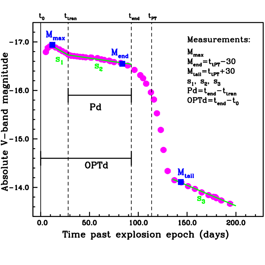
Figure 1.— An example of the light-curve parameters measured for each SN. Observed magnitudes at peak, $M_{\text{max}}$, end of ‘plateau’, $M_{\text{end}}$, and beginning of linear decline, $M_{\text{tail}}$ are shown in blue, as applied to the example dummy data points (magenta). The positions of the three measured slopes: $s_{1}$, $s_{2}$, and $s_{3}$ are shown in green. The time durations: ‘plateau’ length, Pd, and optically thick phase duration, OPTd are indicated in black. Four time epochs are labeled: $t_{0}$, the explosion epoch; $t_{tran}$, the transition from $s_{1}$ to $s_{2}$; $t_{end}$, the end of the optically thick phase; and $t_{PT}$, the mid point of the transition from ‘plateau’ to radioactive tail.

3. Light-curve measurements

In Fig. 1 we show a schematic of the $V$-band light-curve parameters chosen for measurement. On inspection of the light-curves it was immediately evident that many SNe II within the sample show evidence for an initial decline from maximum (which to our knowledge is not generally discussed in detail in the literature , although see Clocchiatti et al. 1996, with respect to SN 1992H), before settling onto a second slower decline rate, normally defined as the plateau. Hence, we proceeded to define and measure two decline rates in the early light-curve evolution, as will be outlined below. For the time origin we employ both the explosion epoch (as estimated by the process outlined in § 3.1) and $t_{\text{PT}}$: the mid-point of the transition between plateau and linear decline epochs obtained through fitting SN II light-curves with the sum of three functions: a Gaussian which fits to the early time peak/decline; a Fermi Dirac function which provides a description of the transition between the plateau and radioactive phases; and a straight line which accounts for the slope due to the radioactive decay (see Olivares E. et al. 2010 for further description). It is important to note here, while the fitting process of $t_{\text{PT}}$ appears to give good objective estimations of the time epoch of transition between plateau and later radioactive phases, its fitting of precise parameters such as decline rates, together with magnitudes and epochs of maximum light is less satisfactory. Therefore, we employ this fitting procedure solely for the measurement of the epoch $t_{\text{PT}}$ (from which other time epochs are defined). In the future, it will be important to build on current template fitting techniques of SNe II light-curves, in order to measure all parameters in a fully automated way. For the current study, we continue as outlined below.
With the above epochs in hand, the measured parameters are:

• $M_{\text{max}}$: defined as the initial peak in the $V$-band light-curve. Often this is not observed, either due to insufficient early time data or poorly sampled photometry. In these cases we take the first photometric point to be $M_{\text{max}}$. When a true peak is observed, it is measured by fitting a low order (four to five) polynomial to the photometry in close proximity to the brightest photometric point (generally $\pm$5 days).
  

• $M_{\text{end}}$: defined as the absolute $V$-band magnitude measured 30 days before $t_{\text{PT}}$. If $t_{\text{PT}}$ cannot be defined, and the photometry shows a single declining slope, then $M_{\text{end}}$ is measured to be the last point of the light-curve. If the end of the plateau can be defined (without a measured $t_{\text{PT}}$) then we measure the epoch and corresponding magnitude manually.
  

• $M_{\text{tail}}$: defined as the absolute $V$-band magnitude measured 30 days after $t_{\text{PT}}$. If $t_{\text{PT}}$ cannot be estimated, but it is clearly observed that the SN has fallen onto the radioactive decline, then $M_{\text{tail}}$ is measured taking the magnitude at the nearest point after transition.
  

• $s_{1}$: defined as the decline rate in magnitudes per 100 days of the initial, steeper slope of the light-curve. This slope is not always observed either because of a lack of early time data, or because of insufficiently sampled light-curves However, in some instances a lack of detection may simply imply a lack of any true peak in the light-curve, together with an intrinsic lack of an early decline phase.
  

• $s_{2}$: defined as the decline rate ($V$-band magnitudes per 100 days) of the second, shallower slope in the light curve. This slope is that referred to in the literature as the ‘plateau’. We note here, there are many SNe within our sample which have light-curves which decline at a rate which is ill-described by the term ‘plateau’. However, in the majority SNe II in our sample (with sufficiently sampled photometry) there is suggestive evidence for a ‘break’ in the light-curve before a transition to the radioactive tail (i.e., an end to a ‘plateau’ or optically thick phase). Therefore, hereafter we use the term ‘plateau’ in quotation marks to refer to this phase of nearly constant decline rate (yet not necessarily a phase of constant magnitude) for all SNe.
  

• $s_{3}$: defined as the linear decline rate ($V$-band magnitudes per 100 days) of the slope reached by each transient after its transition from the previous ‘plateau’ phase. This is commonly referred to in the literature as the radioactive tail.
  

To measure light-curve parameters photometry is analyzed with the curfit package within IRAF. In the case of measurements of $M_{\text{end}}$ and $M_{\text{tail}}$ we interpolate to the desired epoch when $t_{\text{PT}}$ is defined, or define an epoch by eye when this information is not available. $M_{\text{max}}$, as defined above is either the maximum magnitude as defined by fitting a low order polynomial to the maximum of the light-curve (only possible in 15 cases), or is simply taken as the magnitude of the first epoch of $V$-band photometry.
Photometric decline rates are all measured by fitting a straight line to each of the three defined phases, taking into account photometric errors. To measure $s_{1}$ and $s_{2}$ we fit a piecewise linear model with four parameters: the rates of decline (or rise), i.e. the slopes $s_{1}$ and $s_{2}$, the epoch of transition between the two slopes, $t_{\text{tran}}$, and the magnitude offset. This process requires that the start of $s_{1}$ and end of $s_{2}$ are pre-defined, in order to exclude data prior to maximum or once the SN starts to transition to the radioactive tail. The values of $s_{1}$, $s_{2}$ and their transition point are then determined through weighted least squares minimization. We then determine whether the light-curve is better fit with one slope (just $s_{2}$), or both $s_{1}$ and $s_{2}$ using the Bayesian Information Criterion (BIC) (Schwartz, 1978). This statistical analysis uses the best fit chi-square, together with the number of free parameters to determine whether the data are better fit by increasing the slopes from one to two, assuming that all our measurements are independent and follow a Gaussian distribution. It should be noted that although this procedure works extremely well, there are a few cases where one would visually expect two slopes and only one is found. The possible biases of including data where one only measures an $s_{2}$, but where intrinsically there are two slopes, are discussed later in the paper.
Measurements of $s_{3}$ are relatively straight forward, as it is easy to identify when SNe have transitioned to the radioactive tail. Here, we require three data points for a slope measurement, and simply fit a straight line to the available photometry.

3.1. Explosion epoch estimations

While the use of $t_{\text{PT}}$ allows one to measure parameters at consistent epochs with respect to the transition from ‘plateau’ to tail phases, much physical understanding of SNe II rests on having constraints on the epoch of explosion. The most accurate method for determining this epoch for any given SN is when sufficiently deep pre-explosion images are available close to the time of discovery. However, in many cases in the current sample, such strong constraints are not available. Therefore, to further constrain this epoch, matching of spectra to those of a library of spectral templates was used through employing the Supernova Identification (SNID) code (Blondin & Tonry, 2007). The earliest spectrum of each SN within our sample was run through SNID and top spectral matches inspected. The best fit was then determined, which gives an epoch of the spectrum with respect to maximum light of the comparison SN. Hence, using the published explosion epochs for those comparison spectra with respect to maximum light, one can determine an explosion epoch for each SN in the sample. Errors were estimated using the deviation in time between the epoch of best fit to those of other good fits listed, and combining this error with that of the epoch of explosion of the comparison SN taken from the literature for each object.
In the case of SNe with non-detections between 1-20 days before discovery, we use explosion epochs as the mid point between those two epochs, with the error being the explosion date minus the non-detection date. For cases with poorer constraints from non-detections, explosion epochs from the spectral matching outlined above are employed. The validity of this spectral matching technique is confirmed by comparison of estimated epochs with SNe non-detections (where strong constraints exist). Where the error on the non-detection explosion epoch estimation is less than 20 days, the mean absolute difference between the explosion epoch calculated using the non-detection and that estimated using the spectral matching is 4.2 days (for the 61 SNe where this comparison is possible). The mean offset between the two methods is 1.5 days, in the sense that the explosion epochs estimated through spectral matching are on average 1.5 days later than those estimated from non-detections. In the appendix these issues are discussed further, and we show that the inclusion of parameters which are dependent on spectral matching explosion epochs make no difference to our results and conclusions. Finally, we note that a similar analysis was also achieved by Harutyunyan et al. (2008b).

3.2. ‘Plateau’ and optically thick phase durations

A key SN II light-curve parameter often discussed in the literature is the length of the ‘plateau’. This has been claimed to be linked to the mass of the hydrogen envelope, and to a lesser extent the mass of ⁵⁶Ni synthesized in the explosion (Litvinova & Nadezhin, 1985; Popov, 1993; Young, 2004; Kasen & Woosley, 2009; Bersten et al., 2011). Hence, we also attempt to measure this parameter. Before doing so it is important to note how one defines the ‘plateau’ length in terms of current nomenclature in the literature. It is common that one reads that a SN IIP is defined as having ‘plateau of almost constant brightness for a period of several months’. Firstly, it is unclear how many of these types of objects actually exist in nature, as we will show later. Secondly, this phase of constant brightness (or at least constant change in brightness for SNe where significant $s_{2}$ values are measured), should be measured starting after initial decline from maximum, a phase which is observed in a significant fraction of hydrogen rich SNe II (at least in the $V$- and bluer bands).
To proceed with adding clarity to this issue, the start of the ‘plateau’ phase is defined to be $t_{\text{tran}}$ (the $V$-band transition between $s_{1}$ and $s_{2}$ outlined in § 3). The end of the ‘plateau’ is defined as when the extrapolation of the straight line $s_{2}$ becomes 0.1 magnitudes more luminous than the light-curve, $t_{\text{end}}$. This 0.1 mag criterion is somewhat arbitrary, however it ensures that both the light-curve has definitively started to transition from ‘plateau’ to later phases, and that we do not follow the light-curve too far into the transitional phase. Using these time epochs we define two time durations:

• the ‘plateau’ duration: $Pd$ = $t_{\text{end}}$–$t_{\text{tran}}$

• the optically thick phase duration: $OPTd$ = $t_{\text{end}}$–$t_{\text{0}}$

These parameters are labeled in the light-curve parameter schematic presented in Fig. 1. In addition, all derived light-curve parameters: decline rates, magnitudes, time durations, are depicted on their respective photometry in the appendix.

3.3. Extinction estimates

All measurements of photometric magnitudes are first corrected for extinction due to our own Galaxy, using the re-calibration of dust maps provided by Schlafly & Finkbeiner (2011), and assuming an $R_{\rm V}$ of 3.1 (Cardelli et al., 1989). We then correct for host galaxy extinction using measurements of the equivalent width (EW) of sodium absorption (NaD) in low resolution spectra of each object. For each spectrum within the sequence (of each SN), the presence of NaD, shifted to the velocity of the host galaxy is investigated. If detectable line absorption is observed a mean EW from all spectra within the sequence is calculated, and we take the EW standard deviation to be the 1$\sigma$ uncertainty of these values. Where no evidence of NaD is found we assume zero extinction. In these cases, the error is taken to be that calculated for a 2$\sigma$ EW upper limit on the non-detection of NaD. Host galaxy $A_{\rm V}$ values are then estimated using the relation taken from Poznanski et al. (2012), assuming an $R_{\rm V}$ of 3.1 (Cardelli et al., 1989).
The validity of using NaD EW line measurements in low resolution spectra, as an indicator of dust extinction within the host galaxies of SNe Ia has been recently questioned (Poznanski et al. 2011; Phillips et al. 2013). Even in the Milky Way where a clear correlation between NaD EW measurements and $A_{\rm V}$ is observed, the RMS scatter is large. At the same time, absence of NaD is generally a first order approximation of low level or zero extinction, while high EW of NaD possibly implies some degree of host galaxy reddening (Phillips et al., 2013). The use of the Poznanski et al. (2012) relation for the current sample is complicated as it has been shown (e.g. Munari & Zwitter 1997) to saturate for NaD EWs approaching and surpassing 1 Å. Indeed, 10 SNe within the current sample have NaD EWs of more than 2 Å. The Poznanski et al. (2012) relation gives an $A_{\rm V}$ (assuming $R_{\rm V}$ = 3.1) of 9.6 for an EW of 2 Å, i.e. implausibly high. Therefore, we choose to eliminate magnitude measurements of SNe II in our sample with EW measurements higher than 1 Å, due to the uncertainty in any $A_{\rm V}$ corrections. In addition, when measuring 2$\sigma$ upper limits for NaD non-detections, we also eliminate SNe from magnitude analysis if the limits are higher than 1 Å (i.e. spectra are too noisy to detect significant NaD absorption). Finally, those SNe which do not have spectral information are also cut from magnitude analysis.
The above situation is far from satisfying, however for SNe II there is currently no accepted method which accurately corrects for host galaxy extinction. Olivares E. et al. (2010) used the $(V-I)$ color excess at the end of the plateau to correct for reddening, with the assumption that all SNe IIP evolve to similar temperatures at that epoch (see also Nugent et al. 2006; Poznanski et al. 2009; Krisciunas et al. 2009; D’Andrea et al. 2010). Those authors found that using such a reddening correction helped to significantly reduce the scatter in Hubble diagrams populated with SNe IIP. However, there are definite outliers from this trend; e.g. sub-luminous SNe II tend to have red intrinsic colors at the end of the plateau (see e.g. Pastorello et al. 2004; Spiro et al. 2014), which, if one assumed were due to extinction would lead to corrections for unreasonable amounts of reddening (e.g. in the case of SN 2008bk; Pignata private communication). With these issues in mind we proceed, listing our adopted $A_{\rm V}$ values measured from NaD EWs in Table 6.
We note that while the current extinction estimates are uncertain, all of the light-curve relations that will be presented below hold even if we assume zero extinction corrections.

3.4. Distances

Distances are calculated using CMB-corrected recession velocities if this value is higher than 2000 km s^-1, together with an $H_{0}$ of 73 km s^-1 Mpc^-1 (and $\Omega_{m}$ = 0.27, $\Omega_{\Lambda}$ = 0.73, Spergel et al. 2007), assuming a 300 km s^-1 velocity error due to galaxy peculiar velocities. For host galaxies with recession velocities less than 2000 km s^-1 peculiar velocities make these estimates unreliable. For these cases ‘redshift independent’ distances taken from NED are employed, where the majority are Tully-Fisher estimates, but Cepheid values are used where available. Errors are taken to be the standard deviation of the mean value of distances in cases with multiple, e.g. Tully-Fisher values, or in cases with single values the literature error on that value. Distance moduli, together with their associated errors are listed in Table 6.

3.5. Light-curve error estimation

Errors on absolute magnitudes are a combination of uncertainties in: 1) photometric data; 2) extinction estimations and; 3) distances. In 1) when the magnitude is taken from a single photometric point we take the error to be that of the individual magnitude. When this magnitude is obtained through interpolation we combine the errors in quadrature of the two magnitudes used. Published photometric errors are the sum in quadrature of two error components: 1) the uncertainty in instrumental magnitudes estimated from the Poisson noise model of the flux of the SN and background regions, and 2) the errors on the zero point of each image (see Contreras et al. 2010, as applied to the CSP SN Ia sample). In the case of 2) errors in $A_{\rm V}$ are taken as the standard deviation of the mean measurement of the NaD EWs, together with the error on the relation used (Poznanski et al., 2012). However, it is believed that the error on the relation provided by those authors is significantly underestimated. Using the dispersion of individual measurements on the NaD EW-$A_{\rm V}$ relation as seen in Phillips et al. (2013), we obtain an additional error of 47% of $A_{\rm V}$ estimations, which is added to the error budget. In the case of 3) errors for SNe within host galaxies with recession velocities above 2000 km s^-1 are derived from assuming peculiar velocity errors of 300 km s^-1, while for recession velocities below that limit errors are those published along with the distances used (as outlined above). These three errors are combined in quadrature and are listed for each of the three estimated absolute magnitudes in Table 6.
Decline rate uncertainties come from the linear fits to $s_{1}$, $s_{2}$ and $s_{3}$. The uncertainty in $Pd$ is the error on the epoch of the transition between $s_{1}$ and $s_{2}$, as estimated in § 3, while the error on $OPTd$ is that estimated for the explosion epoch, as outlined in § 3.1. We also combine with the uncertainty in $Pd$/$OPTd$, an additional 4.25 days to the error budgets to account for the uncertainty in the definition of $t_{end}$. This error is estimated in the following way. For each SN we calculate the average cadence of photometry at epochs in close proximity to $t_{end}$. The mean of these cadences for all SNe is 8.5 days. Given that $t_{end}$ is measured as an interpolation between photometric points (following $s_{2}$ together with the morphology of the changing light-curve), we assume the error in defining any epoch at this phase to be half the cadence, i.e. 4.25 days.
An additional magnitude error inherent in all SNe measurements is that due to $K$-terms (the wavelength shift of the spectral energy distribution with respect to the observer’s band-pass, Oke & Sandage 1968). For the current analysis we do not make such corrections owing to the low-redshift of our sample. To test this assumption we follow the technique employed in Olivares E. et al. (2010), and described in Olivares (2008). This involved synthesizing $K$-terms from a library of synthetic SN spectra, resulting in a range of corrections as a function of $(B-V)$ SN color. At the mean redshift of our sample of 0.018, the average $K$-correction during the plateau is estimated to be 0.02 mag. At the redshift limit of our sample: 0.077, this mean correction is 0.07 mag. Hence, our neglection of this term is justified. While we also choose to ignore $S$-corrections (magnitude corrections between different photometric systems), we note again that the CSP data are tied to the natural system of the Swope telescope (see Contreras et al. 2010 for details), while all previous data are calibrated to the Landolt standard system. This may bring differences to the photometry of each sub-sample. For a typical SN, the difference in $V$-band magnitudes between photometry in the CSP and standard system is less than 0.1 mag at all epochs (with mean corrections of around 0.03 mag). The differences between $S$-corrections at $M_{\text{max}}$ and $M_{\text{end}}$ are around $\sim$0.03 mag. Therefore the influence of this difference on decline rate estimations will be negligible (they will be less than this difference). In conclusion, uncertainties in our measurements are dominated by those from distances and extinction estimates, and our neglection of these corrections is very unlikely to affect our overall results and conclusions.

3.6. SN II $V$-band light-curves

After correcting $V$-band photometry for both MW and host extinction we produce absolute $V$-band light-curves by subtracting the distance modulus from SNe extinction corrected apparent magnitudes. In Fig. 2 results of Legendre polynomial fits to the absolute light-curves of all those with explosion epochs defined, and $A_{\rm V}$ corrections possible are presented. This shows the large range in both absolute magnitudes and light-curve morphologies, the analysis of which will be the main focus of the paper as presented below. In addition, in the appendix light-curves are presented in more detail for all SNe to show the quality of our data, its cadence, and derived SN parameters. Note that these Legendre polynomial fits are merely used to show the data in a more presentable fashion. They are not used for any analysis undertaken.

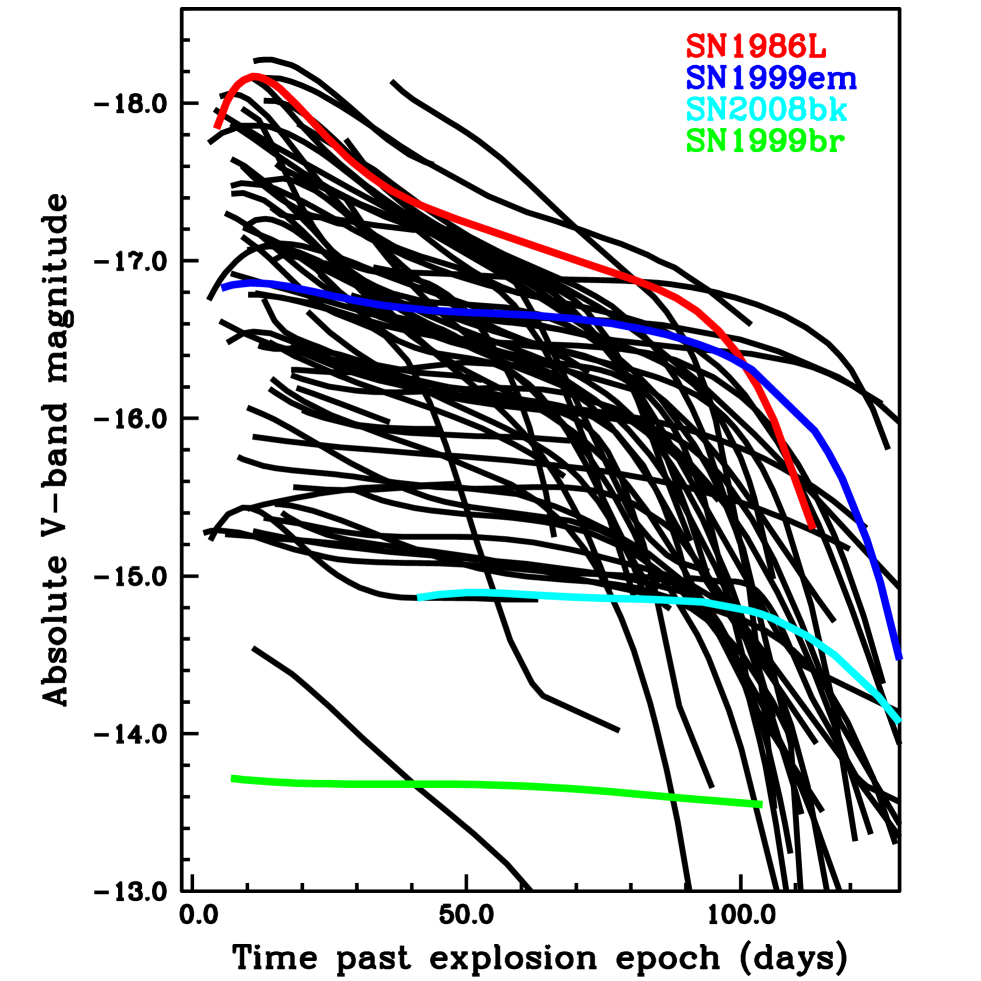
Figure 2.— SNe II absolute $V$-band light-curves of the 60 events with explosion epochs and $A_{\rm V}$ corrections. Light-curves are displayed as Legendre polynomial fits to the data, and are presented by black lines. For reference we also show in colors the fits to our data for 4 SNe II: 1986L, 1999em, 2008bk, and 1999br.

4. Results

In Table 6 we list the measured $V$-band parameters as defined above for each SN, together with the SN distance modulus, host extinction estimate, and explosion epochs. Given eight measured parameters there are a large number of different correlations one can search for and investigate. In this Section figures and statistics of correlations are presented, choosing those we deem of most interest. In the appendix additional figures not included in the main text are presented, which may be of interest.
Throughout the rest of the paper, correlations are tested for significance using the Pearson test for correlation. We employ Monte Carlo bootstrapping to further probe the reliability of such tests. For each of the 10,000 simulations (with random parameter pairs drawn from our measured values) a Pearson’s $r$-value is estimated. The mean $r$ of these 10,000 simulations is then calculated and is presented on each figure, together with its standard deviation. The mean is presented together with an accompanying lower limit to the probability of finding such a correlation strength by chance. Where correlations are presented with parameter pairs ($N$) higher than 20, binned data points are also displayed, with error bars taken as the standard deviation of values within each bin.

4.1. SN II parameter distributions

In Fig. 3 histograms of the three absolute $V$-band magnitude distributions: $M_{\text{max}}$, $M_{\text{end}}$ and $M_{\text{tail}}$ are presented. These distributions evolve from being brighter at maximum, to lower luminosities at the end of the plateau, and further lower values on the tail. Our SN II sample is characterized, after correction for extinction, by the following mean values: $M_{\text{max}}$ = –16.74 mag ($\sigma$ = 1.01, 68 SNe); $M_{\text{end}}$ = –16.03 mag ($\sigma$ = 0.81, 69 SNe); $M_{\text{tail}}$ = –13.68 mag ($\sigma$ = 0.83, 30 SNe).
The SN II family spans a large range of $\sim$4.5 magnitudes at peak, ranging from –18.29 mag (SN 1993K) through –13.77 mag (SN 1999br). At the end of their ‘plateau’ phases the sample ranges from –17.61 to –13.56 mag. SN II maximum light absolute magnitude distributions have previously been presented by Tammann & Schroeder (1990) and Richardson et al. (2002). Both of these were $B$-band distributions. Tammann & Schroeder presented a distribution for 23 SNe II of all types of $M_{\rm B}$ = –17.2 mag ($\sigma$ = 1.2), while Richardson et al. found $M_{\rm B}$ = –17.0 mag ($\sigma$ = 1.1) for 29 type IIP SNe and $M_{\rm B}$ = –18.0 mag ($\sigma$ = 0.9) for 19 type IIL events. Given that our distributions are derived from the $V$ band, a direct comparison to these works is not possible without knowing the intrinsic colors of each SN within both samples. However, our derived $M_{\text{max}}$ distribution is reasonably consistent with those previously published (although slightly lower), with very similar standard deviations.
At all epochs our sample shows a continuum of absolute magnitudes, and the $M_{\text{max}}$ distribution shows a low-luminosity tail as seen by previous authors (e.g. Pastorello et al. 2004; Li et al. 2011). All three epoch magnitudes correlate strongly with each other: when a SN II is bright at maximum light it is also bright at the end of the plateau and on the radioactive tail.

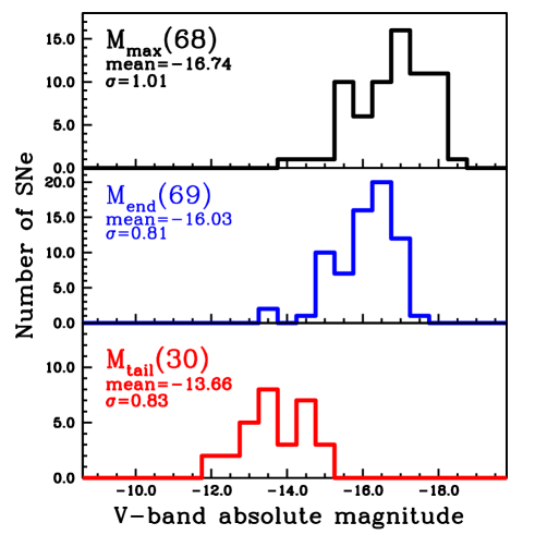
Figure 3.— Histograms of the three measured absolute magnitudes of SNe II. Top: peak absolute magnitudes; $M_{\text{max}}$. Middle: absolute magnitudes at the end of the plateau; $M_{\text{end}}$. Bottom: absolute magnitudes at the start of the radioactive tail; $M_{\text{tail}}$. In each panel the number of SNe is listed, together with the mean absolute $V$-band magnitude and the standard deviation on that mean.

Fig. 4 presents histograms of the distributions of the three $V$-band decline rates, $s_{1}$, $s_{2}$ and $s_{3}$, together with their means and standard deviations. SNe decline from maximum ($s_{1}$) at an average rate of 2.65 mag per 100 days, before declining more slowly on the ‘plateau’ ($s_{2}$) at a rate of 1.27 mag per 100 days. Finally, once a SN completes its transition to the radioactive tail ($s_{3}$) it declines with a mean value of 1.47 mag per 100 days. This last decline rate is higher than that expected if one assumes full trapping of gamma-ray photons from the decay of ⁵⁶Co (0.98 mag per 100 days, Woosley et al. 1989). This gives interesting constraints on the mass extent and density of SNe ejecta, as will be discussed below. We observe more variation in decline rates at earlier times ($s_{1}$) than during the ‘plateau’ phase ($s_{2}$).
As with the absolute magnitude distributions discussed above, the $V$-band decline rates appear to show a continuum in their distributions. The possible exceptions are those SNe declining extremely quickly through $s_{1}$: the fastest decliner SN 2006Y with an unprecedented rate of 8.15 mag per 100 days. In the case of $s_{2}$ the fastest decliner is SN 2002ew with a decline rate of 3.58 mag per 100 days, while SN 2006bc shows a rise during this phase, at a rate of –0.58 mag per 100 days. The $s_{2}$ decline rate distribution has a tail out to higher values, while a sharp edge on the left hand side is seen, with only 6 SNe having negative decline rates during this epoch.
In Fig. 5 we show how the decline rates correlate. A correlation between $s_{1}$ and $s_{2}$ is observed despite a handful of outliers. $s_{2}$ and $s_{3}$ also appear to show the same trend: a fast decliner at one epoch is usually a fast decliner at other epochs. This suggestion that more steeply declining SNe II (during $s_{2}$) also have faster declining radioactive tails was previously suggested by Doggett & Branch (1985). In both of these plots there is at least one obvious outlier: SN 2006Y. We mark the position of this event here and also on subsequent figures where it also often appears as an outlier to any trend observed. Further analysis of this highly unusual event will be the focus of future work.
In summary of the overall distributions of decline rates: SNe II which decline more quickly at early epochs also generally decline more quickly both during the plateau and on the radioactive tail.

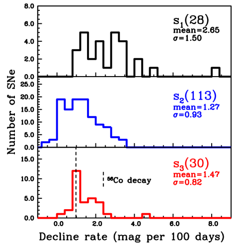
Figure 4.— Histograms of the three measured decline rates of SNe II. Top: initial decline rates from maximum; $s_{1}$. Middle: decline rates on the ‘plateau’ $s_{2}$. Bottom: decline rates on the radioactive tail $s_{3}$. In this last plot a vertical dashed line indicates the expected decline rate for full trapping of emission from ⁵⁶Co decay. In each panel the number of SNe is listed, together with the mean decline rate and the standard deviation on that mean.

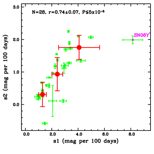
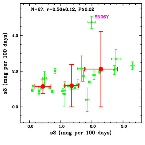
Figure 5.— Correlations between $s_{1}$ and $s_{2}$ (Left), and $s_{2}$ against $s_{3}$ (Right). The results of Monte Carlo simulations on the statistics of these two variables are noted at the top of the figure: $N$ = number of events, $r$ = Pearson’s correlation coefficient, $P$ = probability of detecting a correlation by chance. Binned data are shown in red circles, both here and throughout the paper. The outlier SN 2006Y noted throughout different figures throughout the rest of the paper is shown in magenta.

4.2. Brightness and decline rate correlations

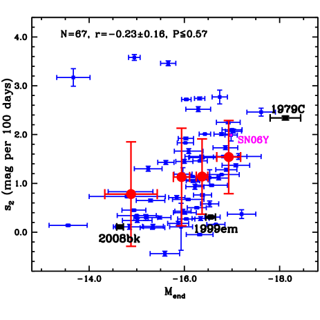
Figure 6.— The magnitude at the end of the ‘plateau’, $M_{\text{end}}$, plotted against the decline rate during the ‘plateau’ $s_{2}$. Individual data points are shown as blue squares. The positions of three individual SNe II are noted: the sub-luminous type IIP, SN 2008bk, the prototype type IIP, SN 1999em (both from our own sample), and the prototype type IIL, SN 1979C (de Vaucouleurs et al., 1981). The results of Monte Carlo simulations on the statistics of these two variables are noted as in Fig. 5.

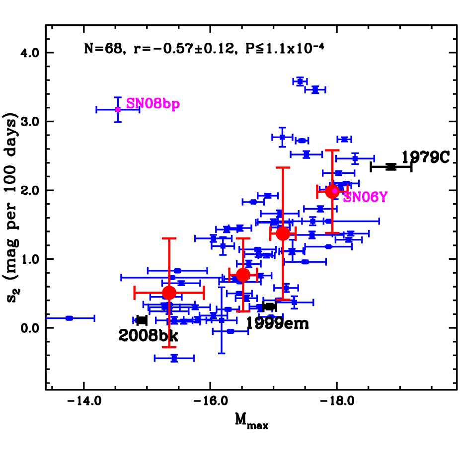
Figure 7.— Peak magnitude, $M_{\text{max}}$, plotted against the decline rate during the ‘plateau’ $s_{2}$. Individual data points are shown as blue squares. The positions of three individual SNe II are noted: the sub-luminous type IIP, SN 2008bk, the prototype type IIP, SN 1999em (both from our own sample), and the prototype type IIL, SN 1979C (de Vaucouleurs et al., 1981). The results of Monte Carlo simulations on the statistics of these two variables are noted as in Fig. 5. SN 2008bp, a major outlier within this correlation is shown in magenta.

Having presented parameter distributions and correlations in the previous Section, here we turn our attention to investigating whether SN brightness and rate of decline of their light-curves are connected. In some of the plots presented in this Section photometric measurements of the prototypical type IIL SN 1979C are also included for comparison (de Vaucouleurs et al. 1981). The positions within the correlations of the prototypical type IIP SN 1999em, plus the sub-luminous type IIP SN 2008bk (both from our own sample) are also indicated.
Given that peak epochs of SNe II are often hard to define, literature measurements of SN II brightness have generally concentrated on some epoch during the ‘plateau’ (e.g. Hamuy 2003a; Nugent et al. 2006). Therefore, we start by presenting the correlation of $M_{\text{end}}$ (brightness at the end of the ‘plateau’) with $s_{2}$ in Fig. 6. No correlation is apparent which is confirmed by a Pearson’s test. Given that $M_{\text{end}}$ does not seem to correlate with decline rates (Fig. 30 shows correlations against $s_{1}$ and $s_{3}$), we move to investigate $M_{\text{max}}$-decline rate correlations.
In Fig. 7 $M_{\text{max}}$ against $s_{2}$ is plotted. It is found that these parameters show a trend with lower luminosity SNe declining more slowly (or even rising in a few cases), and more luminous events declining more rapidly during the ‘plateau’. One possible bias in this correlation is that SNe are included if only one slope is measured (just $s_{2}$) together with those events with two. However, making further cuts to the sample (only including those with $s_{1}$ and $s_{2}$ measurements) does not significantly affect the results and conclusions presented here. Later in § 5.6 we discuss this issue further and show how using a sub-sample of events with both slopes measured enables us to further refine the predictive power of $s_{2}$.
The above finding is consistent with previous results showing that SNe IIL are generally more luminous than SNe IIP (Young & Branch, 1989; Patat et al., 1994; Richardson et al., 2002). It is also interesting to note the positions of the example SNe displayed in Fig. 7: the sub-luminous type IIP SN 2008bk has a low luminosity and a very slowly declining light-curve; the prototype type IIL SN 1979C is brighter than all events in our sample, and also has one of the highest $s_{2}$ values. The prototype type IIP SN 1999em has, as expected, a small $s_{2}$ value, and most (78%) of the remaining SNe II decline more quickly. In terms of $M_{\text{max}}$, on the other hand, SN 1999em does not stand out as a particularly bright or faint object. We note one major outlier to the trend presented in Fig. 7: SN 2008bp with a high $s_{2}$ value (3.17 mag per 100 days) but a very low $M_{\text{max}}$ value (–14.54 mag). It is possible that the extinction has been significantly underestimated for this event based on its weak interstellar absorption NaD, and indeed the SN has a red color during the ‘plateau’ (possibly implying significant reddening). Further analysis will be left for future work.
In Fig. 8 we plot $M_{\text{max}}$ against $s_{1}$. While the significance of correlation is not as strong as seen with respect to $s_{2}$, it still appears that more luminous SNe at maximum light decline more quickly also at early times.
Finally, in Fig. 9 $M_{\text{max}}$ against $s_{3}$ is presented, and the expected decline rate (dashed horizontal line) if one assumes full trapping of gamma-ray photons from the decay of ⁵⁶Co to ⁵⁶Fe is displayed. There appears to be some correlation in that more luminous SNe II at maximum have higher $s_{3}$ values. However, more relevant than a strict one to one correlation, it is remarkable that none of the fainter SNe deviate significantly from the slope expected from full trapping, while at brighter magnitudes significant deviation is observed. The physical implications of this will be discussed below. Finally, we note that while the striking result from Figs 4 and 9 is the number of SNe with $s_{3}$ values higher than 0.98 mag per 100 days, and the fact that nearly all of these are overluminous (compared to the mean) SNe II, it is also observed that there are a number of SNe which have $s_{3}$ values lower than the expected value. These SNe also generally have lower peak luminosities. Indeed this has been noted before, especially for sub-luminous SNe IIP by Pastorello et al. (2009) and Fraser et al. (2011). In the case of SN 1999em, Utrobin (2007) argued that the discrepancy (from the rate expected due to radioactivity) was due to radiation from the inner ejecta propagating through the external layers and providing additional energy (to that of radioactivity) to the light-curve, naming this period the ‘plateau tail phase’.

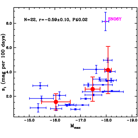
Figure 8.— Peak magnitude $M_{\text{max}}$, plotted against the initial decline rate $s_{1}$. Individual data points are shown as blue squares. The results of Monte Carlo simulations on the statistics of these two variables are noted as in Fig. 5.

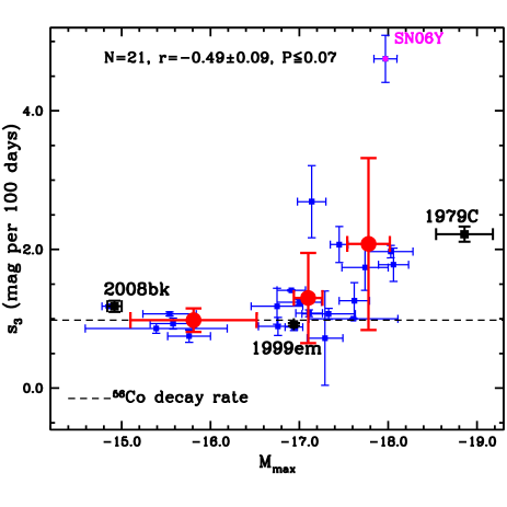
Figure 9.— SN peak magnitudes, $M_{\text{max}}$, plotted against the decline rate during the radioactive tail $s_{3}$. Individual data points are shown as blue squares. The dashed horizontal line shows the expected decline rate on the radioactive tail, assuming full trapping of gamma-rays from ⁵⁶Co to ⁵⁶Fe decay. The positions of three different SNe II are noted: the sub-luminous type IIP, SN 2008bk, the prototype type IIP, SN 1999em (both from our own sample), and the prototype type IIL, SN 1979C (de Vaucouleurs et al., 1981). The results of Monte Carlo simulations on the statistics of these two variables are noted as in Fig. 5.

4.3. Plateau duration

In Fig. 10 both the $V$-band ‘plateau’ duration ($Pd$) distribution, together with its correlation with $M_{\text{max}}$ are displayed. A large range of $Pd$ values is observed, from the shortest of $\sim$27 days (again the outlier SN 2006Y discussed above) to the longest of $\sim$72 days (SN 2003bl), with no signs of distribution bimodality. The mean $Pd$ for the 19 events where a measurement is possible is 48.4 days, with a standard deviation of 12.6. While statistically there is only small evidence for a trend, it is interesting to note that the two SNe with the longest $Pd$ durations are also of low-luminosity, while that with the shortest $Pd$ is one of the most luminous events.
In Fig. 11 both the $V$-band optically thick phase duration ($OPTd$) distribution, together with its correlation with $M_{\text{max}}$ are displayed. Again, a large range in values is observed with a mean $OPTd$ of 83.7 days, and $\sigma$= 16.7. The mean error on estimated $OPTd$ values is 7.8$\pm$3.0 days. Hence, the standard deviation of $OPTd$ values is almost twice as large as the typical error on any given individual SN. This argues that the large range in observed $OPTd$ values is a true intrinsic property of the analyzed sample. The shortest duration of this phase is SN 2004dy with $OPTd$= 25 days, while the largest $OPTd$ is for SN 2004er, of 120 days. SN 2004dy is a large outlier within the OPTd distribution, marking it out as a very peculiar SN. Further comment on this will be left for future analysis, however we do note that Folatelli et al. (2004) observed strong He i emission in the spectrum of this event, also marking out the SN as spectroscopically peculiar. Again, within the $OPTd$ distribution there appears to be a continuum of events. Although there is no statistical evidence for a correlation between the $OPTd$ and $M_{\text{max}}$, the most sub-luminous events have some of the longest $OPTd$, while those SNe with the shortest $OPTd$ durations are more luminous SNe II. These large continuous ranges in $Pd$ and $OPTd$ are in contrast to the claims of Arcavi et al. (2012) who suggested that all SNe IIP have ‘plateau’ durations of $\sim$100 days (however we note that the Arcavi et al. study investigated $R$-band photometry, rather than the $V$-band data presented in the current work). Further comparison of the current results to those of Arcavi et al. will be presented below.
In Fig. 12 correlations between both $Pd$ and $OPTd$ with $s_{2}$ are presented. While there is much scatter in the relations, these results are consistent with the picture of faster declining SNe II having shorter duration ‘plateau’ phases (see e.g. Blinnikov & Bartunov 1993). Indeed, such a trend was first observed by Pskovskii (1967). A similar, but stronger trend is observed when $Pd$ and $OPTd$ are correlated against $s_{1}$, as presented in Fig. 13
Finally, in Fig. 14 we present correlations between $Pd$ and $OPTd$ with $s_{3}$. As will be discussed in detail below, both $OPTd$ and $s_{3}$ provide independent evidence for significant variations in the mass of the hydrogen envelope/ejecta mass at the epoch of explosion. The trend shown in Fig. 14 in that SNe with longer $OPTd$ values have smaller $s_{3}$ slopes, is consistent with the claim that such variations can be attributed to envelope mass.
In summary, generally SNe which have shorter duration $Pd$ and $OPTd$ tend to decline more quickly at all epochs.

Figure 10.— Top panel: histogram of distribution of $Pd$. Bottom panel: $Pd$ against $M_{\text{max}}$. (Note, in the histogram there are more events than in the correlation due to the removal of those SNe without constrained extinction values from the correlation). The results of Monte Carlo simulations on the statistics of these two variables are noted as in Fig. 5. in magenta.

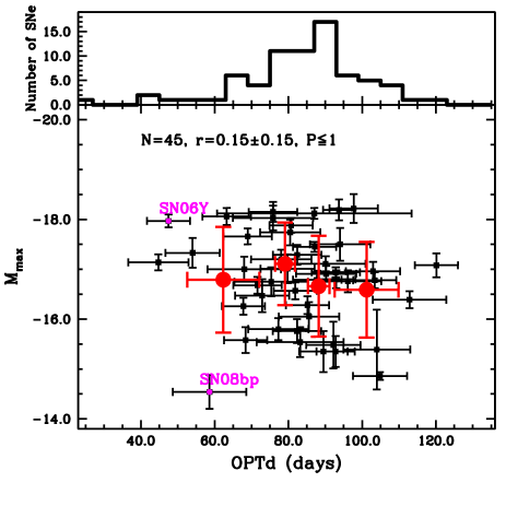
Figure 11.— Top panel: histogram of $OPTd$. Bottom panel: $OPTd$ against $M_{\text{max}}$. (Note, in the histogram there are more events than in the correlation due to the removal of those SNe without constrained extinction values from the correlation). The results of Monte Carlo simulations on the statistics of these two variables are noted as in Fig. 5. In addition, the outlier in Fig. 7: SN 2008bp is also seen as an outlier in this plot.

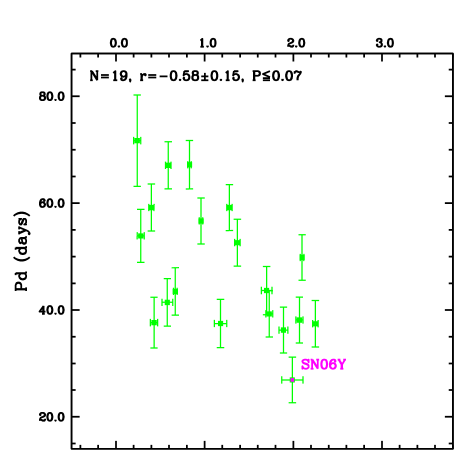
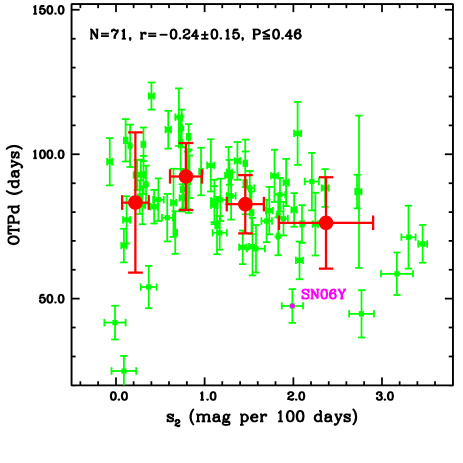
Figure 12.— Top panel: SN ‘plateau’ durations ($Pd$) plotted against $s_{2}$. Bottom panel: SN optically thick durations ($OPTd$) plotted against $s_{2}$. The results of Monte Carlo simulations on the statistics of these two variables are noted as in Fig. 5.

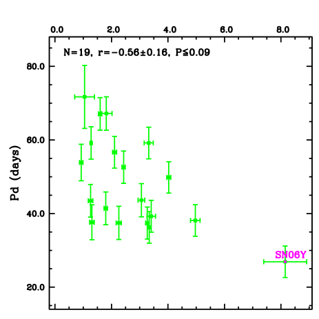
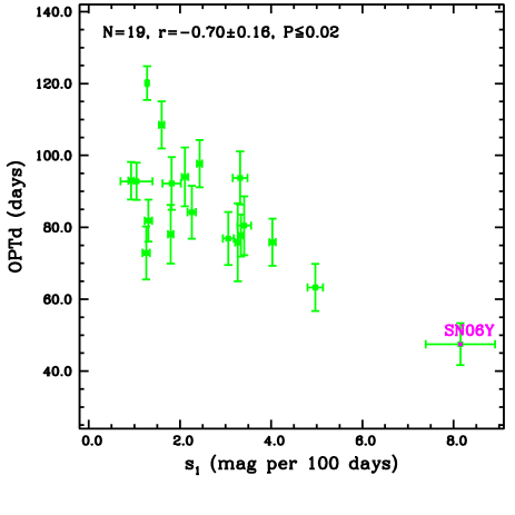
Figure 13.— Top panel: SN ‘plateau’ durations ($Pd$) plotted against $s_{1}$. Bottom panel: SN optically thick durations ($OPTd$) plotted against $s_{1}$. The results of Monte Carlo simulations on the statistics of these two variables are noted as in Fig. 5.

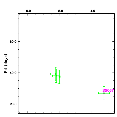
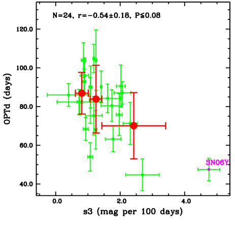
Figure 14.— Top panel: SN ‘plateau’ durations ($Pd$) plotted against $s_{3}$. Bottom panel: SN optically thick durations ($OPTd$) plotted against $s_{3}$. The results of Monte Carlo simulations on the statistics of these two variables are noted as in Fig. 5.

4.4. ⁵⁶Ni mass estimates

Given that the exponential tail (phase $s_{3}$) of the SN II light-curves are presumed to be powered by the radioactive decay of ⁵⁶Co (see e.g. Woosley 1988), one can use the brightness at these epochs to determine the mass of ⁵⁶Ni synthesized in the explosion. However, as we have shown above, there is a significant spread in the distribution of $s_{3}$ values, implying that not all gamma-rays released during to the decay of ⁵⁶Co to ⁵⁶Fe are fully trapped by the ejecta during the exponential tail, rendering the determination of the ⁵⁶Ni mass quite uncertain. Therefore, we estimate ⁵⁶Ni masses only in cases where we have evidence that $s_{3}$ is consistent with the value expected for full trapping (0.98 mag per 100 days). For all other SNe with magnitude measurements during the tail, but either $s_{3}$ values significantly higher (0.3 mag per 100 days higher) than 0.98 (mag per 100 days), or SNe with less than three photometric points (and therefore no $s_{3}$ value can be estimated), lower limits to ⁵⁶Ni masses are calculated. In addition, for those SNe without robust host galaxy extinction estimates (see § 3.3) we also calculate lower limits.
To estimate ⁵⁶Ni masses and limits, the procedure presented in Hamuy (2003a) is followed. $M_{\text{tail}}$ $V$-band magnitudes are converted into bolometric luminosities using the bolometric correction derived by Hamuy et al. (2001), together with the distance moduli and extinction values reported in Table 6. Given our estimated explosion epochs, mass estimates are then calculated and are listed in Table 6.
In Fig. 15 we compare $OPTd$ and ⁵⁶Ni masses. Young (2004) and Kasen & Woosley (2009) claimed that heating from the radioactive decay of ⁵⁶Ni should further extend the plateau duration. We do not find evidence for that trend in the current sample (consistent with the finding of Bersten 2013). In fact, if any trend is indeed observed it is the opposite direction to that predicted.
The range of ⁵⁶Ni masses is from 0.007${\rm\ M}_{\odot}$ (SN 2008bk) to 0.079${\rm\ M}_{\odot}$ (SN 1992af), and the distribution (shown in Fig. 15) has a mean value of 0.033 ($\sigma$= 0.024)${\rm\ M}_{\odot}$. Given the earlier trends observed between $s_{3}$ and other parameters it is probable that there is a systematic effect, and those SNe II where only lower limits are possible are probably not simply randomly distributed within the rest of the population. Therefore, we caution that this ⁵⁶Ni synthesized mass distribution is probably biased compared to the true intrinsic range.

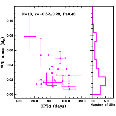
Figure 15.— Left: $OPTd$ against derived ⁵⁶Ni masses. Right: Distribution of ⁵⁶Ni masses (lower mass limits are not included in the figure). (Note, in the histogram there are more events than in the correlation, due to the removal of those SNe without constrained $OPTd$ values). The results of Monte Carlo simulations on the statistics of these two variables are noted as in Fig. 5.

4.5. Transition steepness

Elmhamdi et al. (2003) reported a correlation between the steepness of $V$-band light-curves during the transition from plateau to tail phases (named the inflection time in their work), and estimated ⁵⁶Ni masses. With the high quality data presented in the current work, we are in an excellent position to test this correlation. The Elmhamdi et al. method entailed weighted least squares minimization fitting of a defined function (their equation 1), to the $V$-band light-curve in the transition from plateau to radioactive phases in the period of $\pm$50 days around the inflection point of this transition. The steepness parameter is then defined as the point at which the derivative of magnitude with time is maximal. We attempt this same procedure for all SNe in the current sample. We find that it is possible to define a reliable steepness ($S$) term in only 21 cases. This is because one needs extremely well sampled light curves at epochs just before, during and after the transition. Even for well observed SNe this type of cadence is uncommon, and we note that in cases where one can define an $S$-value, additional data points at key epochs could significantly change the results. We do not find any evidence for a correlation as seen by Elmhamdi et al., and there does not appear to be any trend that could be used for cosmological purposes to standardize SNe II light-curves (see the appendix for further details).

5. Discussion

Using the $V$-band light-curve parameters as defined in § 3 and displayed in Fig. 1 we have presented a thorough characterization of 116 SN II light curves, both in terms of morphologies and absolute magnitudes, and explored possible correlations among parameters. Our main result is that SNe II which are brighter at maximum light ($M_{\text{max}}$) decline more quickly at all three phases of their $V$-band light-curve evolution. In addition, our data imply a continuum of $V$-band SN II properties such as absolute magnitude, decline rates, and length of the ‘plateau’ and optically thick phase durations. In this Section we further discuss the most interesting of our results, in comparison to previous observational and theoretical SN II work, and outline possible physical explanations to explain the diversity of SN II events found.

5.1. $M_{\text{max}}$ as the dominant brightness parameter

$M_{\text{max}}$ shows the highest degree of correlation with decline rates of all defined SN magnitudes. From an observational point of view this is maybe somewhat surprising, given the difficultly in defining this parameter: a true maximum is often not observed in our data, and hence in the majority of cases we are forced to simply use the first photometric point available for our estimation. This uncertainty in $M_{\text{max}}$ indeed implies that the intrinsic correlation between $M_{\text{max}}$ and the two initial decline rates, $s_{1}$ and $s_{2}$, is probably even stronger. Paying close attention to Fig. 7 together with Fig. 27, it is easy to see why this could be the case. In general a low-luminosity SN has a slow decline rate at both initial and ‘plateau’ epochs. Therefore, if one were to extrapolate back to the ‘true’ $M_{\text{max}}$ magnitude, its measured value would change very little. However, this is not the case for the most luminous SNe. In general these have much faster declining light-curves. Hence, if we extrapolate these back to their ‘true’ peak values, these SNe will have even brighter $M_{\text{max}}$ values, and hence the strength of the correlation could be even higher than that presently measured.
The statement that faster declining SNe (type IIL) are brighter than slower declining ones (type IIP) is not a new result. This has been seen previously in the samples of e.g. Pskovskii (1967); Young & Branch (1989); Patat et al. (1994) and Richardson et al. (2002). However, (to our knowledge) this is the first time that a wide-ranging correlation as shown in Fig. 7 has been presented with the supporting statistical analysis.

5.2. A continuum of SN II properties in the $V$-band

Arcavi et al. (2012) recently claimed that SNe IIP and SNe IIL appear to be separated into two distinct populations in terms of their $R$-band light-curve behavior, possibly suggesting distinct progenitor scenarios in place of a continuum of events. In the current paper we have made no attempt at definitive classifications of events into SNe IIP and SNe IIL (ignoring whether such an objective classification actually exists). However, in the above presented distributions and figures we see no evidence for a separation of events into distinct categories, or a suggestion of bimodality. While it is important to note that these separate analyses were undertaken using different optical filters, these results are intriguing.
In Fig. 16 Legendre polynomial fits to all light-curves of SNe with explosion epoch constraints are presented, the same as in Fig. 2, but now with all SNe normalized to $M_{\text{max}}$, and also including SNe where host extinction corrections were not possible. While this figure shows the wide range in decline rates and light-curve morphologies discussed above, there does not appear to be any suggestion of a break in morphologies. Given all of the distributions we present, together with the qualitative arguments of Fig. 16, it is concluded that this work implies a continuum of hydrogen-rich SNe II events, with no clear separation between SNe IIP and SNe IIL (at least in the $V$ band).
To further test this suggestion of an observational continuum, in Fig. 17 we present the same light-curves as in Fig. 16, but now presented as a density plot. This is achieved in the following way. Photometry for each SN was interpolated linearly to the time interval of each bin (which separates the overall time axis into 20 bins). This estimation starts with the first bin where the first photometric point lies for each SN, and ends at the bin containing the last photometric point used to make Fig. 16. This interpolation is done in order to compensate for data gaps and to homogenize the observed light-curve to the given time intervals. In Fig. 16 it is hard to see whether there are certain parts of the light-curve parameter space that are more densely populated than others, given that light-curves are simply plotted on top of one another. If the historically defined SNe types IIP and IIL showed distinct morphologies, then one may expect such differences to be more easily observed in a density plot such as that presented in Fig. 17. However, we do not observe any such well defined distinct morphologies in Fig. 17 (although we note that even the large sample of more than 100 SN light-curves is probably insufficient to elucidate these differences through such a plot). In conclusion, Fig. 17 gives further weight to the argument that in the currently analyzed sample there is no evidence for multiple distinct $V$-band light-curve morphologies, which clearly separate SNe IIP from SNe IIL.
The suggestion of a large scale continuum derived from our analysis is insightful for the physical understanding of hydrogen-rich explosions. A continuum could imply that the SN II population is formed by a continuum of progenitor properties, such as ZAMS mass, with the possible conclusion that more massive progenitors lose more of their envelopes prior to explosion, hence exploding with lower mass envelopes, producing faster evolving light-curves than their lower progenitor mass companions. We note that the claim of a continuum of properties for explaining differences in hydrogen-rich SNe II light-curves is also supported by previous modeling from e.g. Blinnikov & Bartunov (1993). These authors suggest that the diversity of events could be explained through differing pre-SNe radii, the power of the pre-SN wind, and the amount of hydrogen left in the envelope at the epoch of explosion.

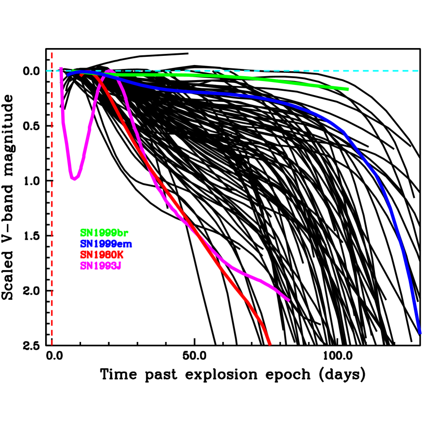
Figure 16.— A continuum of SNe II $V$-band light-curve morphologies. Similar to Fig. 2, however here magnitudes are normalized to peak SN magnitudes, and we also include SNe where host extinction corrections were not possible. For reference, fits to the data of SN 1980K (Buta 1982; Barbon et al. 1982, as no explosion date estimate is available for this event, we assume an epoch of 10 days before the first photometric point), SN 1999em and SN 1999br are displayed in colored lines. In addition, we show a fit to the $V$-band light-curve of the type IIb, SN 1993J (Richmond et al., 1994).

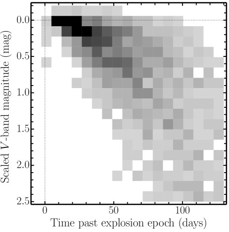
Figure 17.— 2d density histogram of the normalized light-curves presented in Fig. 16. Photometry is interpolated to the time intervals of the grid, which separate the light-curve parameter space into $20\times 20$ bins.

5.3. A lack of true ‘linear’ SNe II?

In the process of this work it has been noted that there is no clear objective classification system for defining a SN IIP from a SN IIL. The original classification was made by Barbon et al. (1979) who from $B$-band light curves, stated that (1) SNe IIP are characterized by a rapid decline, a plateau, a second rapid decline, and a final linear phase, which in our terminology correspond to $s_{1}$, $s_{2}$, transition between ‘plateau’ and tail phases (the mid point being $t_{\text{PT}}$), and $s_{3}$ respectively; (2) SNe IIL are characterized by an almost linear decline up to around 100 days post maximum light (also see Doggett & Branch 1985). This qualitative classification then appears to have been used for the last 3 decades without much discussion of its meaning or indeed validity. A ‘plateau’ in the truest sense of the word would imply something that does not change, in this case the light-curve luminosity remaining constant for a period of at least a few months. However, if we apply this meaning to the current sample, claiming that anything which changes at a rate of less than 0.5 magnitudes per 100 days during $s_{2}$ is of SN IIP class, then this includes only $\sim$25% of SNe II in the current sample, much less than the percentages of 75% and 95% estimated by Li et al. (2011) and Smartt et al. (2009) respectively (or the 65% in the original publication of Barbon et al. 1979). Even if we relax this criterion to 1 magnitude per 100 days, then still only 41% of the current sample would be classified as SNe IIP.
Meanwhile, as outlined above, the generally accepted terminology for SNe IIL appears to be that these events have fast linear decline phases post maximum until they evolve to the radioactive tail. However, it is unclear how many SNe actually exist either in the literature or within our own sample which fulfill this criterion. Two literature prototype type IIL events are SN 1979C and SN 1980K. However, while both of these SNe have relatively fast declining light-curves, they both show evidence for an end to their ‘plateau’ phases, or ‘breaks’ in their light-curves (i.e. an end to $s_{2}$ or the optically thick phase, before transition to $s_{3}$). This is shown in Fig. 18, where the $V$-band photometry for both objects (data from de Vaucouleurs et al. 1981 and Buta 1982; Barbon et al. 1982 respectively) are plotted, together with the data for the three SNe within our sample which have the highest $s_{2}$ values. In the case of four of the five SNe plotted in Fig. 18 there is evidence for a ‘break’ in the light-curves, i.e. an end to an $s_{2}$ phase, while in the remaining case the data are insufficient to make an argument either way. (We note that in the case of SN 1979C one observes a smooth transition between phases, more than a sharp change in light-curve shape, while in the case of SN 2003ej the evidence for a ‘break’ is supported by only one data point after the $s_{2}$ decline).
It could be that SNe IIL are not solely those that evolve the quickest, but those where there is no evidence for a ‘plateau’ or ‘break’ in their light-curves. Therefore, we visually search through our sample attempting to identify those SNe which are most likely to be classified as SNe IIL in the historically defined terminology. Only six cases are identified, together with SN 2002ew already presented in Fig. 18, and their $V$-band light-curves are displayed in Fig. 19. This figure shows some interesting features. At least half of the SNe displayed show signs of a maximum around 10-20 days post explosion, a characteristic that is rare in the full SN II sample. After early epochs it would appear that these events could be defined as having ‘linear’ morphologies. However, there are two important caveats before one can label these as SNe IIL in the historical sense: 1) none of the seven SNe presented in Fig. 19 has photometry after day 100 post explosion (with only 2 SNe having data past 80 days), hence it could be that a ‘break’ before the radioactive tail is merely unobserved due to the lack of late time data, and 2) for about half of the events the cadence at intermediate epochs is such that one may have simply missed any ‘break’ phase during these epochs. Putting these caveats aside, even if we assume that these 7 events should be classified as SNe IIL, this would amount to a relative fraction of SNe IIL events in the current sample of $\sim$6% (of hydrogen rich SNe II), i.e. at lowest limit of previously estimated percentages (Barbon et al., 1979; Smartt et al., 2009; Li et al., 2011). Hence, we conclude that if one uses the literal meaning of the historically defined SNe IIL class, then these events are intrinsically extremely rare.

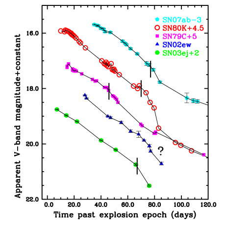
Figure 18.— $V$-band light-curves of the two prototypical SNe IIL: 1979C (de Vaucouleurs et al., 1981) and 1980K (Buta, 1982; Barbon et al., 1982), together with light-curves of the 3 SNe within our sample with the highest $s_{2}$ values: SNe 2002ew, 2003ej and 2007ab. On each light-curve we indicate where there is a possible ‘break’ (at the end of $s_{2}$), before the SN transitions to the radioactive tail (for SN 2002ew a ’?’ indicates that any such epoch is unclear).

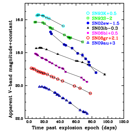
Figure 19.— Seven SNe II $V$-band light-curves taken from our sample to be the most probable SNe IIL events.

5.4. Light-curve classifications of SNe II

Given the arguments presented in the previous two sub-sections: a continuum of events; no clear separation between the historically defined SNe IIP and SNe IIL; a possible lack of any true steeply declining ‘linear’ SNe II; many SNe having much faster declining light-curves than the prototypical type IIP SN 1999em, we believe that it is time for a reappraisal of the SN II light-curve classification scheme. Indeed, the current terminology in the literature, and its use by different researchers prohibits consistent statistical analyses and gives virtually no quantitative information on light-curve morphology. It is therefore proposed that given the easiest parameter to measure for any given SN II is the decline rate during the ‘plateau’ phase, its $s_{2}$ value, that this parameter should be used to define any given SN II. This would follow the similar procedure of SN Ia classifications, where individual events are further classified by referring to their $\bigtriangleup$m₁₅ value (decline in brightness during the first 15 days post maximum light, Phillips 1993b) or ‘stretch’ parameter (Perlmutter et al., 1997). Hence, we propose that to standardize terminology, future SNe II are referred to as e.g. ‘SN1999em, a SN II with $s_{2}$= 0.31’. This will enable investigators to define SN samples in a consistent manner which is not currently possible. This is particularly pertinent for future surveys (such as that of the Large Synoptic Survey Telescope, LSST, Ivezic et al. 2008) which will produce thousands of SNe II light-curves and where simply referring to a SN as type IIP or type IIL gives little quantitative information. Using a standardized terminology will allow one to define e.g. a range of SNe II which are good standard candles, i.e. possibly only those traditionally classified as SNe IIP. However, now one could quantify this by giving a sample range of e.g. $-0.5<s_{2}<1$.

5.5. Physical interpretations of SN II $V$-band light-curve diversity

5.5.1 The prevalence of $s_{1}$: extended cooling in SNe II?

While many historical SNe II have been published with sufficient data to observe the initial maximum and decline from maximum (see e.g. SN 1999em photometry published in Hamuy et al. 2001 and Leonard et al. 2002), the initial $s_{1}$ decline rate has attracted little attention in SN II discussion (although its presence was indeed noted in the original SN II classification publication of Barbon et al. 1979, and was discussed in more detail for the case of SN 1992H by Clocchiatti et al. 1996). In the current work we have objectively measured $s_{1}$ values for 28 SNe or $\sim$24% of our sample, while there is visual evidence for such slopes in many more SNe. Physically, this initial steeper decline phase is most probably related to the remaining early-time cooling following shock break-out (i.e. related to the early-time declining bolometric light-curve: see e.g. Grassberg et al. 1971; Falk & Arnett 1977). The extent in time, post explosion of this cooling is predicted to be directly related to the radius of the pre-SN progenitor star (see Bersten et al. 2012, for recent application of this hypothesis to a SN IIb). It is therefore intriguing to note that these $s_{1}$ durations continue for several weeks post explosion. It is also interesting that the $s_{1}$ distribution spans a wide range in decline rates, and shows trends with $Pd$ and $OPTd$ as displayed in Fig. 13. A full analysis of early-time bolometric light-curves of CSP and literature SNe, and their comparison to model light-curves, together with the implications for progenitor properties is underway.

5.5.2 Probing ejecta/envelope properties with $s_{3}$ and $OPTd$

Prior to this work, it has generally been assumed that the decline rates of the majority of SNe II at late times follow that predicted by the decay of ⁵⁶Co, at least until 300-400 days post explosion (see e.g. Young 2004 for predictions of deviations at very late times). Indeed this was claimed to be the case in Patat et al. (1994) (although see Doggett & Branch 1985 for a suggestion that faster declining SNe have late time light-curves which deviate from those expected). This has been based on the assumption that SNe II have sufficiently massive and dense ejecta to fully trap the radioactive emission. However, as seen in Fig. 4 there are significant deviations from the expected decay rate of $s_{3}$= 0.98 mag per 100 days, at epochs only $\sim$80-150 days post explosion. Indeed, 10 of the 30 SNe II with measured $s_{3}$ have values significant higher than 0.98 mag per 100 days (we note the caveat that these observational measurements are in the $V$ band, while theoretical expected rates are for bolometric magnitudes). In the most extreme cases there is a SN with an $s_{3}$ value higher than 3 mag per 100 days (SN 2006Y). This suggests that in these cases the ejecta mass and/or density are too low for full trapping of the gamma-ray emission resulting from the decay of ⁵⁶Co. Given that $s_{3}$ shows significant correlation with $s_{2}$ (which can be used as a proxy to differentiate between ‘plateau’ and ‘linear’ SNe), this would appear to be direct evidence that faster declining SNe II have smaller mass and less dense ejecta, as suggested/predicted (see e.g. Blinnikov & Bartunov 1993).
While a detailed analysis and discussion of ejecta masses and densities implied by the above arguments is beyond the scope of this paper, the above results and discussion of $s_{3}$ and its correlations with other light-curve parameters implies that in a significant fraction of SNe II explosions the mass and/or density of the ejecta are significantly smaller than previously assumed, thus allowing early leakage of gamma-ray emission.
The hydrogen envelope mass at the epoch of explosion has been claimed to directly influence the optically thick phase duration (see Chevalier 1976; Litvinova & Nadezhin 1983, 1985; Popov 1993). The standard historical picture is that as normal SNe IIP transition to more linear events, the subsequent SNe have shorter, less pronounced ‘plateau’/optically thick phases (indeed the SN 1992H; Clocchiatti et al. 1996, is likely to be an example of such a transitional event). This is shown in Fig. 12, where there is marginal evidence for a trend in that more steeply declining SNe have smaller $Pd$ and $OPTd$ values implying that more ‘linear’ events have smaller envelope masses at the time of explosion. The large range in $OPTd$ values implies that SNe II explode with a large range of masses of retained hydrogen envelopes.

5.5.3 Mass extent and density profile of SNe II as the dominant physical parameter

Following the previous discussion, it appears that the majority of diversity observed in SN II light-curves and indeed their spectra (see below) can be described through varying the extent (in mass and density profile) of hydrogen envelopes retained prior to SN explosion. This is obviously a simplified picture and there are other properties which will play a role, such as explosion energy, pre-SN radius, and synthesized ⁵⁶Ni mass. However, we suggest that the results of the above presented analysis are most easily explained by differing hydrogen masses. Indeed, this would be completely consistent with the SNe II model parameter space study of Young (2004), who investigated the influence on the light-curve properties of varying the progenitor radius, envelope mass, explosion energy, ⁵⁶Ni mass, and the extent of the mixing of the synthesized ⁵⁶Ni. Young concluded that the primary parameter (together with progenitor radius) that affects the overall behavior of SNe II light-curves, and can explain their observed diversity is the observed hydrogen envelope mass at explosion epoch. He predicted that decreasing the hydrogen envelope at the epoch of explosion would lead to a number of changes in the light-curve properties. Firstly, a larger mass envelope leads to a longer diffusion time, and hence radiation is trapped for a longer time, leading to less luminous early time light-curves and flatter ‘plateau’ phases (i.e. lower $s_{2}$ values). Secondly, a smaller mass leads to shorter duration plateaus (or $OPTd$) as the recombination wave has less mass to travel back through. Finally, a reduced hydrogen envelope leads light-curve tails to be steeper (higher $s_{3}$ values), which is the result of leakage of radioactive emission. This can be seen in our analysis as presented in Figs 4 and 14 (although we note the caveat that deviation of $s_{3}$ values occur at much earlier times in our data than that predicted). We also note that Dessart et al. (2013) analyzed the dependencies of SN IIP radiation on progenitor and explosion properties. They found that explosions with higher kinetic energies lead to SNe with brighter and shorter plateau phases. While that study did not analyze the effects of changes to the hydrogen envelope mass, Hillier et al. (in preparation) have included such changes, finding that explosions with lower envelope masses indeed are brighter, have faster declining light-curves with shorter ‘plateau’ phases, consistent with our conclusions here (Dessart 2013 private communication).
If the above hypothesis is true, together with our claim of a continuum of SN II properties, then the next question becomes: how do different progenitors evolve to produce this diversity in final hydrogen envelope profiles? The dominant process would appear to be the mass loss history of each progenitor. The degree of mass loss suffered by high mass stars is influenced by progenitor properties such as ZAMS mass, metallicity, binarity and rotation (with mass loss rates increasing for increasing mass and metallicity, and the presence of a close binary companion accelerating the process). However, to date there are few constraints on how these parameters change with respect to the diversity of events observed. Progenitor mass constraints have been most accurately determined through direct detection of progenitor stars on pre-explosion images. Smartt et al. (2009) derived a progenitor mass range for SNe IIP of 8-16${\rm\ M}_{\odot}$. However, the upper limits of this range has been questioned by Walmswell & Eldridge (2012) due to the effects of circumstellar dust (although see Kochanek et al. 2012), and in addition, Fraser et al. (2012) and Maund et al. (2013) have published detections of more recent SNe IIP, suggesting higher masses for two further events. In the case of SNe IIL there have been a couple of progenitor detections, with suggestions that these could indeed arise from higher zero age main sequence (ZAMS) mass progenitor stars than SNe IIP (e.g. Elias-Rosa et al. 2010, 2011). This would then be consistent with faster declining SNe II losing a higher degree of their envelopes prior to explosion, through stronger mass-loss due to their more massive ZAMS progenitors, and hence their light-curve behavior being similar to that presented above (also consistent with the fact that historical SNe IIL, e.g. SN 1980K, SN 1979C, have also been strong radio emitters, Weiler et al. 1989). This picture is also supported by work on the environments of CC SNe, where SNe IIL show a higher degree of association to host galaxy on-going star formation (as traced by H$\alpha$ emission) than their SNe IIP counterparts (Anderson et al., 2012). Changes in progenitor metallicity (see Dessart et al. 2014 for discussion on how progenitor metallicities may be directly probed from SN spectra), binarity and rotation remain relatively unconstrained, but are also likely to affect the transient behavior and diversity of SNe II events.
Finally, at this stage it is important to mention the spectral analysis currently being achieved on the same sample analyzed here. Gutiérrez et al. (submitted) are focusing on the profile of the dominant H$\alpha$ P-Cygni profiles of hydrogen-rich SNe II events. In that paper it is shown that the events we discuss here as being bright, having steeply declining light-curves, and shorter duration phases, also in general have less prominent P-Cygni absorption features with respect to emission (together with higher H$\alpha$ measured velocities), a characteristic which again is likely to be linked to smaller mass hydrogen envelopes at the epoch of explosion (see e.g. Schlegel 1996). Anderson et al. (submitted) have also shown that the strength of the blueshift of the peak of emission of H$\alpha$ correlates with both $s_{2}$ and $M_{\text{max}}$, in the sense that brighter and faster declining SNe II have higher blue-shifted velocities than their dimmer, slower declining counterparts.

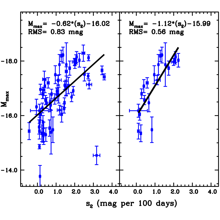
Figure 20.— Correlations between $s_{2}$ and $M_{\text{max}}$. Left The full sample as displayed earlier in Fig. 7. Right SNe II which have measured $s_{1}$ and $s_{2}$ values. In each figure the line of best fit, estimated through Monte Carlo bootstrapping is presented, together with the linear relation between $s_{2}$ and $M_{\text{max}}$, and the RMS dispersion in magnitudes of the derived relations.

5.6. SNe II as photometric standardizable candles?

SNe II (or specifically SNe IIP) have long been discussed as complementary (to SNe Ia) distance indicators, with a number of techniques being employed to standardize their luminosities (e.g. the expanding photosphere method, EPM: Kirshner & Kwan 1974; Eastman et al. 1996; Dessart & Hillier 2005; Dessart et al. 2008; jon09;bos14, the spectral fitting expanding photosphere method, SEAM: Mitchell et al. 2002; Baron et al. 2004, and the standard candle method, SCM: Hamuy & Pinto 2002; Nugent et al. 2006; Poznanski et al. 2009; D’Andrea et al. 2010; Olivares E. et al. 2010). However, a key issue that currently precludes their use for higher redshift cosmology is the need for spectral measurements in these techniques. Any photometric relation between SN II luminosities and other parameters, if found could enable SNe II to be used as accurate high-redshift distance indicators. This would be particularly pertinent when one keeps pushing to higher redshift where the SN Ia rate is expected to drop due to their relative long progenitor lifetimes, while the SNe II rate should remain high as it follows the star formation rate of the Universe.
In Fig. 7 a correlation between $M_{\text{max}}$ and $s_{2}$ was presented, where more luminous events show steeper declining light-curves. In Fig. 20 we now invert the axis of the earlier figure in order to evaluate the predictive power of $s_{2}$. The best fit line is estimated by running 10,000 Monte Carlo bootstrap simulations and calculating the mean of the slopes and y-intercept values obtained. This then leads to a relation between $s_{2}$ and $M_{\text{max}}$ for the full sample, as presented in the left panel of Fig. 20, which has a dispersion of 0.83 mag. However, it was earlier noted in § 4.2 that in this full sample we are including SNe where only a measurement of $s_{2}$ was possible (i.e. no distinction between $s_{1}$ and $s_{2}$). This may bias the sample, as if an $s_{1}$ is not detected but intrinsically is present, then it will merge with $s_{2}$, and probably artificially increase the value of $s_{2}$ we present in Table 6. Following this we make a cut to our sample to only include SNe where both the measurement of $s_{1}$ and $s_{2}$ are favored (see § 3). We then obtain a sample of 22 events. The correlation between $s_{2}$ and $M_{\text{max}}$ for this curtailed sample is stronger: running our Monte Carlo simulated Pearson’s test gives, $r=-0.82\pm 0.05$ and $P\leq 3\times 10^{-5}$. In the right panel of Fig. 20 this correlation is presented, and the following relation is derived:

• $M_{\text{max}}=-1.12(s_{2})-15.99$

This relation has a dispersion of only 0.56 mag. While this is still higher than that published for SN II spectroscopic distance methods (and considerably higher than SN Ia), the predictive power of $s_{2}$ is becoming very promising. If the accuracy of parameters such as host galaxy extinction can be improved, and SN color information included, then it may be possible to bring this dispersion down to levels where SNe II are indeed viable photometric distance indicators, independent of spectroscopic measurements.
A model correlation between the SN luminosity at day 50 post explosion (closest to our $M_{\text{end}}$ value) and the duration of the plateau was predicted by Kasen & Woosley (2009) (see also Bersten 2013), which they claimed could (if corroborated by observation) be used to standardize SNe IIP luminosities. We only observe marginal evidence for any such trends.

5.7. Future SNe II studies

While statistical studies of SNe II as that presented here are to date rare or even non-existent, they promise to become much more prevalent in the near future, with larger field of view and deeper transient searches planned or underway. During the course of this investigation it has become obvious that a number of key attributes are needed to efficiently further our understanding of hydrogen-rich SNe II through well planned observations. Firstly, strong constraints on the explosion epoch is key, as this allows measurements to be derived with respect to a well defined epoch (in the case of SNe Ia one can use the maximum of the light-curve, however for SNe II such a method contains higher levels of uncertainty). Secondly, high cadence photometry is warranted to be able to differentiate between different slopes such as $s_{1}$ and $s_{2}$. Indeed, it appears that it is often assumed that SNe IIP light-curves are reasonably well behaved and therefore one can obtained photometry in a more relaxed fashion. However, it is clear from the current work that photometry obtained every few days is needed to further our understanding of the diversity of SNe II: in general one does not know at what stage a SN II will transition from one phase to the other, and data at those points are vital for the phases to be well constrained. Thirdly, detailed observations of the radioactive tails are needed to confirm and further investigate deviations from $s_{3}$ values expected from full trapping. Such observations contain direct information on the ejecta profiles of each SN and are key to understanding the progenitor and pre-SN properties of SNe II. While the current study has opened many avenues for further investigation and intriguing insights to the underlying physics of SNe II explosions, continued high quality data are needed to deepen our understanding of hydrogen-rich SNe II. As we have hinted throughout this paper, the CSP has obtained multi-color optical and near-IR light-curves, together with high quality spectral sequences of a large sample of SNe II. The near-IR data could prove key to the understanding of SNe II, and their use as distance indicators, since they are essentially unaffected by dust extinction. The full analysis of those samples will present a large increase in our understanding of the observational diversity of SNe II events.

6. Conclusions

An analysis of $V$-band photometry of 116 SNe II has been presented with the aim of characterizing the diversity seen within their light-curves. This has been achieved through defining three magnitude measurements at different epochs: $M_{\text{max}}$, $M_{\text{end}}$, $M_{\text{tail}}$, three photometric decline rates: $s_{1}$, $s_{2}$ and $s_{3}$, together with the time durations $Pd$ and $OPTd$. We analyzed these distributions, and searched for possible correlations. Our main findings are that the SN II family forms a continuum of events in terms of their light-curve morphologies (in the $V$ band), and that while large dispersion is observed, brighter SNe at maximum generally decline more quickly at all epochs. We speculate that the majority of the diversity of SNe II can be explained through differences in their hydrogen envelope masses at the epoch of explosion, a parameter which is most directly measured through observations of the optically thick phase duration ($OPTd$). Finally, we list our main conclusions originating from this work.

• A continuum of SN II $V$-band properties is observed in all measured parameters (absolute magnitudes, decline rates, optically thick phase durations), and we observe no clear bimodality or separation between the historically defined SNe IIP and SNe IIL.

• SNe which are brighter at maximum decline more quickly at all epochs.

• After making a series of data quality cuts, it is found that the dispersion in the relation between $s_{2}$ and $M_{\text{max}}$ can be reduced to 0.56 mag, which opens the way to using SNe II as photometric distance indicators, independent of spectroscopic information.

• While $M_{\text{max}}$ is more difficult to define and measure than other magnitudes, it shows the highest degree of correlation with decline rates. Hence, it appears that $M_{\text{max}}$ is the dominant magnitude parameter describing the diversity of SNe II.

• We find a large range in $V$-band optically thick, and ‘plateau’ durations ($OPTd$, $Pd$) which implies a large range in hydrogen envelope masses at the epoch of explosion. The fact that these parameters show correlation with a number of other light-curve parameters suggests that one of the most dominant physical parameters that explains the diversity of SNe II light-curves is the envelope mass at the epoch of explosion.

• There are a significant number of SNe II which decline more quickly during the radioactive tail, $s_{3}$, than the rate expected through full trapping of gamma-ray emission. This implies a large range in ejecta masses, with many SNe II having low mass/density ejecta, through which emission can escape.

• Given the qualitative nature of current discussion in the literature of different SNe II, we suggest the introduction of a new parameter, $s_{2}$: the decline rate per 100 days of the $V$-band light-curve during the ‘plateau’ phase. This will enable future studies to make quantitative comparisons between SNe and SNe samples in a standardized way.

• The historically defined SN IIL class does not appear to be significantly represented within this sample, and therefore it is concluded that truly ‘linearly’ declining hydrogen-rich SNe II are intrinsically extremely rare events.

• SN II $V$-band magnitudes show a dispersion at the end of the ‘plateau’, $M_{\text{end}}$ of 0.81 mag, 0.2 mag lower than that at peak, $M_{\text{max}}$.

In the above main body of this manuscript we have tried to present a broad overview of our analysis and resulting conclusions, without discussing every correlation or avenue of investigation that formed part of this SN II light-curve exploration. For completeness, in this appendix several more figures are presented to further elaborate on this theme, and provide further examples of the methods used throughout the work earlier discussed. Finally, Table 6 presents values for all measured parameters for the full SN sample.

Table 2Spectoscopic classification information of the SN II sample

SN	Classification	N. of spectra	Earliest and	Comments
	reference		latest epochs
1986L	Lloyd Evans et al. (1986)	28	+6, +118	Spectra analyzed in Hamuy (2003a)
1991al	Bouchet et al. (1991)	8	+30, +125	Spectra analyzed in Hamuy (2003a); Olivares E. et al. (2010)
1992ad	McNaught et al. (1992)	0	$\cdots$	Classification from circular
1992af	della Valle & Bianchini (1992)	5	+22, +136	Spectra analyzed in Hamuy (2003a); Olivares E. et al. (2010)
1992am	Phillips et al. (1992)	2	$\cdots$	Spectra published in Schmidt et al. (1994),
				and further analyzed in Hamuy (2003a); Olivares E. et al. (2010)
1992ba	Evans & Phillips (1992)	8	+9, +180	Spectra analyzed in Hamuy (2003a); Jones et al. (2009); Olivares E. et al. (2010)
1993A	Phillips (1993a)	2	+20, +103	Spectra analyzed in Hamuy (2003a); Olivares E. et al. (2010)
1993K	Hamuy (1993a)	10	+13, +363
1993S	Hamuy (1993b)	4	+35, +94	Spectra analyzed in Hamuy (2003a)
1999br	Garnavich et al. (1999)	8	+16, +75	Spectra analyzed in Hamuy (2003a); Jones et al. (2009); Olivares E. et al. (2010),
				Literature data published in Pastorello et al. (2004)
1999ca	Patat et al. (1999)	4	+28, +41	Spectra analyzed in Hamuy (2003a); Olivares E. et al. (2010)
1999cr	Maza et al. (1999)	5	+11, +57	Spectra analyzed in Hamuy (2003a); Olivares E. et al. (2010)
1999eg	Jha et al. (1999b)	2	+27, +61	Spectra analyzed in Hamuy (2003a)
1999em	Jha et al. (1999a)	7	+10, +168	Spectra published in Hamuy et al. (2001), and further
				analyzed in Hamuy (2003a); Jones et al. (2009); Olivares E. et al. (2010).
				Literature data published in Baron et al. (2000); Leonard et al. (2002)
0210	$\cdots$	6	+56, +87	Spectra analyzed in Hamuy (2003a)
2002ew	Chornock et al. (2002b),	7	+30, +76
	Filippenko & Chornock (2002)
2002fa	Hamuy (2002b)	6	+27, +74	Spectra analyzed in Olivares E. et al. (2010)
2002gd	Hamuy (2002a)	12	+4, +97
2002gw	Hamuy et al. (2002)	11	+14, +91	Spectra analyzed in Jones et al. (2009); Olivares E. et al. (2010)
2002hj	Chornock et al. (2002a)	7	+24, +86	Spectra analyzed in Olivares E. et al. (2010)
2002hx	Matheson et al. (2002)	9	+25, +121	Spectra analyzed in Olivares E. et al. (2010)
2002ig	Miknaitis et al. (2002)	5	+17, +64	Spectra indicate hydrogen-rich type II event
2003B	Kirshner & Silverman (2003)	9	+24, +282	Spectra analyzed in Olivares E. et al. (2010)
2003E	Hamuy (2003d)	8	+15, +131	Spectra analyzed in Olivares E. et al. (2010)
2003T	Foley et al. (2003)	6	+20, +111	Spectra analyzed in Jones et al. (2009); Olivares E. et al. (2010)
2003bl	Phillips et al. (2003)	8	+3, +96	Spectra analyzed in Jones et al. (2009); Olivares E. et al. (2010)
2003bn	Salvo et al. (2003b)	12	+13, +127	Spectra analyzed in Jones et al. (2009); Olivares E. et al. (2010)
2003ci	Salvo et al. (2003b)	5	+19, +87	Spectra analyzed in Olivares E. et al. (2010)
2003cn	Hamuy (2003b)	5	+11, +79	Spectra analyzed in Olivares E. et al. (2010)
2003cx	Hamuy (2003c)	6	+12, +93	Spectra analyzed in Olivares E. et al. (2010)
2003dq	Phillips & Hamuy (2003)	3	+34, +64
2003ef	Ganeshalingam et al. (2003)	6	+31, +107	Spectra analyzed in Jones et al. (2009); Olivares E. et al. (2010)
2003eg	Ganeshalingam et al. (2003)	5	+17, +99
2003ej	Matheson et al. (2003b)	3	+15, +41
2003fb	Papenkova et al. (2003)	4	+22, +96	Spectra analyzed in Olivares E. et al. (2010)
2003gd	Kotak et al. (2003)	3	+51, +141	Spectra analyzed in Olivares E. et al. (2010), literature
				data published in Hendry et al. (2005)
2003hd	Hamuy et al. (2003)	9	+10, +133	Spectra analyzed in Olivares E. et al. (2010)
2003hg	Elias-Rosa et al. (2003)	5	+25, +108	Spectra analyzed in Olivares E. et al. (2010)
2003hk	Filippenko et al. (2003)	4	+34, +104	Spectra analyzed in Olivares E. et al. (2010)
2003hl	Filippenko et al. (2003)	6	+34, +129	Spectra analyzed in Jones et al. (2009); Olivares E. et al. (2010)
2003hn	Salvo et al. (2003a)	9	+32, +175	Spectra analyzed in Jones et al. (2009); Olivares E. et al. (2010),
				and data published in Krisciunas et al. (2009)
2003ho	Hamuy & Roth (2003)	5	+43, +120
2003ib	Morrell & Hamuy (2003)	5	+11, +77
2003ip	Filippenko et al. (2003)	4	+33, +94	Spectra analyzed in Olivares E. et al. (2010)
2003iq	Matheson et al. (2003a)	5	+10, +78	Spectra analyzed in Jones et al. (2009); Olivares E. et al. (2010)
2004dy	Filippenko et al. (2004),	3	+14, +21, +27	Noisy spectra, however clear ‘plateau’ in light-curve
	Folatelli et al. (2004)
2004ej	Folatelli et al. (2004)	9	+38, +134
2004er	Modjaz et al. (2004)	10	+31, +175
2004fb	Morrell et al. (2004)	4	+60, +101
2004fc	Salvo et al. (2004b)	10	+13, +124
2004fx	Salvo et al. (2004a)	10	+23, +110	Data published in Hamuy et al. (2006)
2005J	Modjaz et al. (2005)	11	+23, +97
2005K	Modjaz et al. (2005)	2	+40, +44	Clear ‘plateau’ shaped light-curve
2005Z	Morrell et al. (2005c)	9	+12, +82
2005af	Filippenko & Foley (2005)	9	+110, +176
2005an	Modjaz et al. (2005)	7	+15, +50	Spectra indicate hydrogen-rich type II event

Table 3Spectoscopic classification information of the SN II sample.

SN	Classification	N. of spectra	Epochs of spectra	Comments
	reference
2005dk	Morrell et al. (2005a)	5	+40, +100
2005dn	Morrell et al. (2005a)	6	+38, +98
2005dt	Serduke et al. (2005)	1	+34	Light-curve indicates ‘plateau’ classification
2005dw	Serduke et al. (2005)	3	+36, +121	Spectra indicate hydrogen-rich type II event
2005dx	Serduke et al. (2005)	1	+14	Light-curve indicates ‘plateau’ classification
2005dz	Stanishev et al. (2005)	5	+20, +108
2005es	Morrell et al. (2005b)	1	+14	Noisy spectrum, light-curve indicates probable ‘plateau’
2005gk	Ganeshalingam et al. (2005)	0	$\cdots$	Clear ‘plateau’ shaped light-curve
2005hd	Antilogus et al. (2005)	0	$\cdots$	Clear ‘plateau’ shaped light-curve
2005lw	Hamuy et al. (2005)	11	+5, +134
2005me	Leonard (2005)	1	+72
2006Y	Morrell & Folatelli (2006)	10	+13, +85	Spectra indicate hydrogen-rich type II event
2006ai	Morrell & Folatelli (2006)	7	+17, +68	Spectra indicate hydrogen-rich type II event
2006bc	Patat et al. (2006a)	3	+9, +31	Literature data published in Gallagher et al. (2012)
2006be	Patat et al. (2006b)	4	+19, +45
2006bl	Blondin et al. (2006)	3	+18, +28
2006ee	Foley et al. (2006)	6	+42, +94
2006it	Sahu & Anupama (2006)	4	+10, +36
2006iw	Morrell et al. (2006a)	4	+8, +77
2006ms	Morrell et al. (2006b)	3	+15, +28
2006qr	Silverman et al. (2006)	7	+20, +94
2007P	Blondin & Tonry (2007)	4	+21, +86	Spectra indicate hydrogen-rich type II event
2007U	Blondin et al. (2007b)	7	+8, +75
2007W	Foley et al. (2007)	7	+14, +95
2007X	Folatelli & Morrell (2007)	10	+6, +88
2007aa	Folatelli et al. (2007)	9	+15, +96
2007ab	Blondin et al. (2007c)	5	+40, +84
2007av	Harutyunyan et al. (2007)	4	+10, +56
2007hm	Buton et al. (2007)	6	+20, +86	Spectra indicate hydrogen-rich type II event
2007il	Blondin et al. (2007a)	9	+12, +95
2007it	Contreras et al. (2007)	8	+6, +244	Literature data published in Andrews et al. (2011)
2007ld	Bassett et al. (2007)	6	+4, +38	Spectra indicate hydrogen-rich type II event
2007oc	Olivares & Folatelli (2007)	9	+20, +64
2007od	Blondin & Calkins (2007a)	7	+6, +42	Literature data published in Inserra et al. (2011)
2007sq	Blondin & Calkins (2007b)	4	+31, +100
2008F	Blondin & Berlind (2008)	2	+12, +21	Noisy spectra and photometry
2008K	Stritzinger et al. (2008a)	9	+9, +109
2008M	Folatelli et al. (2008)	10	+19, +97
2008W	Stritzinger & Folatelli (2008)	8	+24, +123
2008ag	Stritzinger & Folatelli (2008)	14	+30, +137
2008aw	Dennefeld et al. (2008)	10	+20, +98	Spectra indicate hydrogen-rich type II event
2008bh	Barth et al. (2008)	6	+10, +55
2008bk	Morrell & Stritzinger (2008)	22	+26, +268	Literature data published in Van Dyk & Matheson (2012)
2008bm	Stritzinger & Morrell (2008)	4	+41, +79	Originally classified as type IIn, however spectrum shows
				clear H$\alpha$ absorption, and light-curve is of ‘plateau’ morphology.
				Narrow lines are most likely related to underlying star
				formation region (as indicated by 2d spectrum)
2008bp	Stritzinger & Morrell (2008)	4	+12, +88
2008br	Morrell & Stritzinger (2008)	4	+13, +43
2008bu	Covarrubias & Morrell (2008)	5	+12, +36
2008ga	Steele et al. (2008)	3	+55, +110
2008gi	Stritzinger et al. (2008b)	5	+11, +81
2008gr	Stritzinger et al. (2008c)	3	+27, +63
2008hg	Harutyunyan et al. (2008a)	4	+11, +31
2008ho	Stanishev & Uthas (2008)	2	+18, +23	Spectra indicate hydrogen-rich type II event
2008if	Challis & Berlind (2008)	17	+11, +136
2008il	Stritzinger (2008a)	3	+3, +63
2008in	Challis (2008),	10	+7, +122	Literature data published in Roy et al. (2011)
	Foley (2008),
	Stritzinger (2008b)

Table 3Spectoscopic classification information of the SN II sample.

SN	Classification	N. of spectra	Epochs of spectra	Comments
	reference
2009N	Challis & Berlind (2009b)	11	+24, +128	Spectra published in Takáts et al. (2014)
2009ao	Stritzinger et al. (2009)	5	+28, +62
2009au	Stritzinger et al. (2009)	7	+24, +80	Originally classified as type IIn, however spectrum shows
				clear H$\alpha$ absorption, and light-curve is of ‘plateau’ morphology.
				Narrow lines are most likely related to underlying star
				formation region (as indicated by 2d spectrum)
2009bu	Morrell & Stritzinger (2009)	6	+12, +67
2009bz	Challis & Berlind (2009a)	4	+9, +37	Spectra indicate hydrogen-rich type II event

Appendix A Sample characterization

As noted in § 1, the currently analyzed sample is an eclectic mix of SNe II, discovered by many different SN search campaigns, of both professional and amateur nature. In this Section, we further characterize the SN and host galaxy samples, and briefly discuss some possible consequences of their properties.
Fig. 21 presents a pie chart which shows the contributions of various SN programs and individuals to the discovery of SNe presented in this analysis. The largest number of events included, discovered by any one survey/individual are those reported by the Lick Observatory Supernova Search (LOSS/LOTOSS, Leaman et al. 2011), who contribute 41 SNe ($\sim$40%). Surprisingly, the next highest contributor to our sample is Berto Monard, an amateur astronomer from South Africa, with an impressive 12 entries ($\sim$10%). Next is the CHilean Automatic Supernova sEarch (CHASE, Pignata et al. 2009) with 11, followed by ‘Maza’ (SNe discovered by investigators at Universidad de Chile during the 1990s, led by Jose Maza), Robert Evans (another amateur astronomer, from Australia), and the NEAT survey (Near-Earth Asteroid Tracking). All other discoveries are grouped into ‘Other’. The vast majority of SNe were discovered by galaxy targeted surveys (88%, counting SDSS, CSS, and NEAT as non-targeted surveys). As most targeted surveys are biased towards bright nearby galaxies, this may lead to a bias against SNe in low-luminosity host galaxies. These and similar issues are discussed for the LOSS SN sample in Li et al. (2011).
In Fig. 22 we present the host galaxy recession velocity and absolute $B$-band magnitude distributions respectively. Our sample has a mean recession velocity of 5505 km s^-1, equating to a mean redhift of 0.018, and a mean distance of 75 Mpc, with the vast majority of galaxies having velocities lower than 10000 km s^-1. The host galaxy population is characterized as having a well defined absolute magnitude $B$-band peak at $\sim$–21 mag, together with a low luminosity tail down to around –17 mag. Host galaxy absolute magnitudes are listed in Table 1. It is interesting to compare this heterogeneous sample with that published by Arcavi et al. (2010) (CC SNe discovered by the Palomar Transient Factory: PTF). While those authors published host galaxy $r$-band magnitudes (compared to the $B$-band magnitudes analyzed here), overall the distributions appear qualitatively similar, with the exception that the PTF sample has a much more pronounced lower-luminosity tail. If the intrinsic rate of specific SNe II events changes with host galaxy luminosity (due to e.g. a dependence on progenitor metallicity), then this could affect the overall conclusions draw from our sample, where we are possibly missing SNe in low-luminosity hosts. A full analysis of these host galaxy properties is beyond the scope of this paper, and a detailed host galaxy study of the CSP sample is underway.

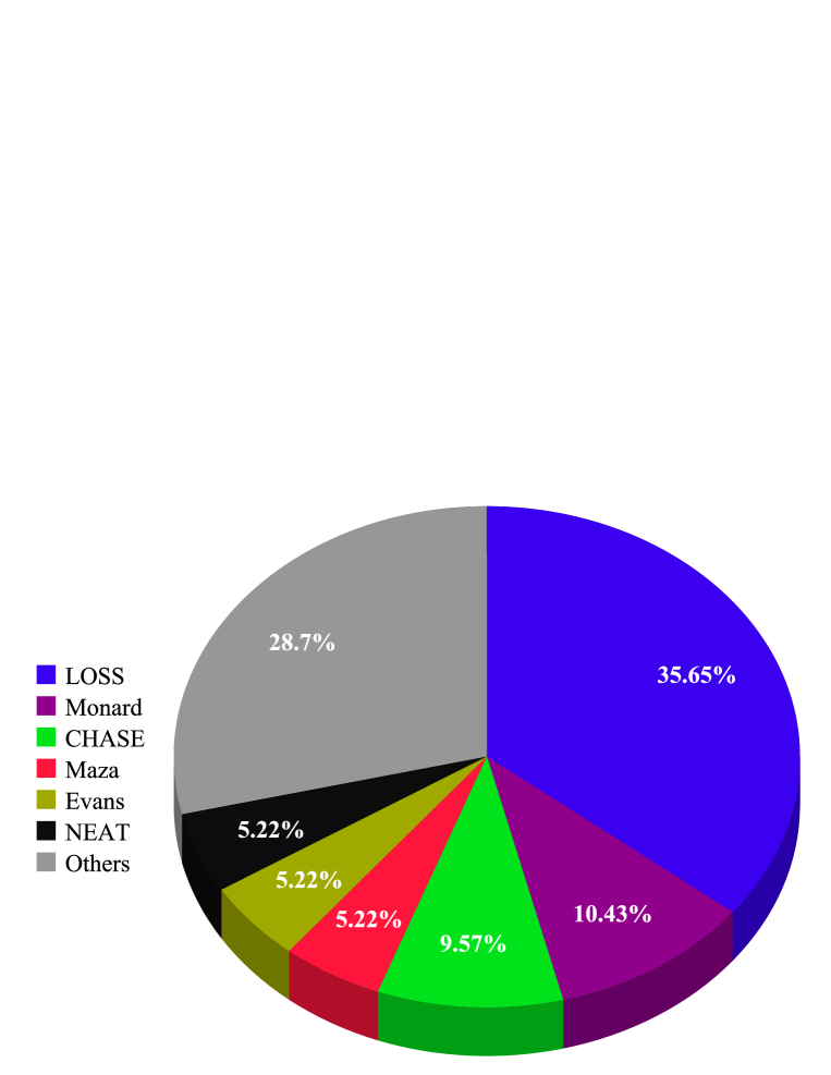
Figure 21.— Pie chart of the relative contributions of different SN search campaigns to the SN II sample analyzed in this publication. Contributions with more than 5 entries are shown individually, while the rest are grouped into ‘Others’ (which includes SNe discovered the following programs/individuals: ‘CROSS’; Yamagata; Itagaki; ‘CSS/CRTS’; ‘Brazil’; Mikuz; Arbour; Doi; Boles; ‘SN factory’; Brass; Lulin; Llapasset; ‘Tenagra’; ‘SDSS’; Puckett; Hurst; ‘Perth’). The entry ‘Maza’ refers to those SNe discovered by investigators at Universidad de Chile during the 1990s.

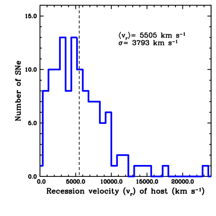
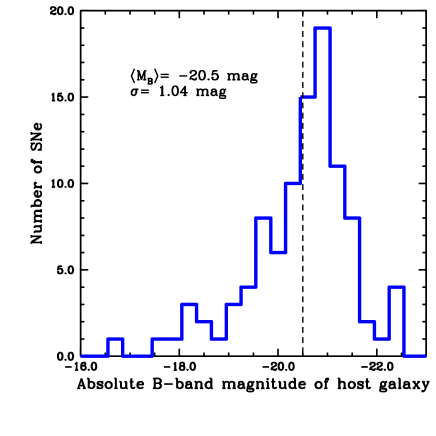
Figure 22.— Left: histogram of the heliocentric recession velocities of the host galaxies of the SNe included in the current sample. Right: histogram of the absolute $B$-band magnitudes of the host galaxies of the SNe included in the current sample (taken from the LEDA database)

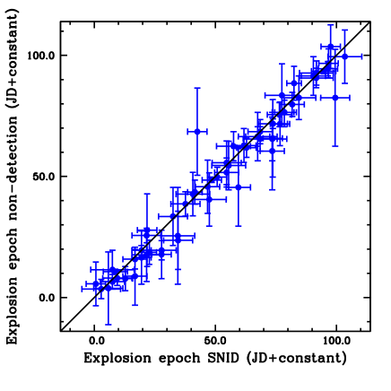
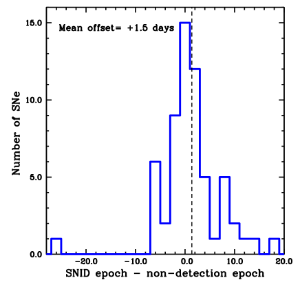
Figure 23.— Left: comparison of the explosion dates estimated through spectral matching (x-axis) and through SN non-detection on pre-discovery images (y-axis). The straight line shows a one-to-one relation between the two epoch estimation methods. Right: histogram of the offsets between explosion epochs estimated through both methods. The mean offset in days between the two estimation methods is indicated by the dashed vertical line.

Table 3Explosion epoch comparisons.

SN	Spectral matching	Non-detection	Difference (days)
	explosion epoch (MJD)	explosion epoch (MJD)
1986L	46710(6)	46708(3)	2
1993K	49074(6)	49066(9)	8
1999br	51279(4)	51277(4)	2
1999ca	51278(7)	51284(13)	–6
1999em	51479(5)	51477(5)	2
2002fa	52501(7)	52500(11)	4
2002gw	52560(5)	52546(16)	14
2002hj	52558(7)	52563(6)	–5
2002hx	52585(7)	52583(9)	2
2003E	52635(7)	52626(20)	9
2003T	52656(7)	52655(10)	1
2003bn	52697(4)	52695(3)	2
2003ci	52708(9)	52712(8)	–4
2003cn	52720(4)	52717(11)	3
2003eg	52774(5)	52761(16)	13
2003ej	52777(5)	52776(5)	1
2003hg	52869(7)	52866(5)	3
2003hl	52869(5)	52869(5)	0
2003hn	52868(8)	52867(10)	1
2003ho	52848(7)	52841(11)	7
2003ib	52891(5)	52883(16)	8
2003iq	52920(4)	52920(2)	0
2004er	53274(6)	53272(2)	2
2004fb	53243(4)	53269(18)	–26
2004fc	53295(5)	53294(1)	1
2004fx	53303(8)	53304(4)	–1
2005Z	53397(4)	53397(6)	0
2005dk	53600(6)	53583(20)	17
2005dt	53601(4)	53606(9)	–5
2005dw	53598(4)	53604(9)	–6
2005dz	53628(6)	53620(4)	8
2005es	53638(6)	53639(5)	–1
2005lw	53717(10)	53709(12)	8
2005me	53722(6)	53718(11)	4
2006Y	53768(5)	53767(4)	1
2006be	53806(6)	53804(15)	2
2006ee	53963(4)	53962(4)	1
2006it	54008(5)	54007(3)	1
2006iw	54009(5)	54011(1)	–2
2006ms	54033(6)	54034(12)	–1
2006qr	54062(5)	54063(7)	–1
2007P	54123(3)	54119(5)	4
2007U	54135(6)	54124(12)	11
2007il	54351(4)	54350(4)	1
2007it	54349(4)	54349(1)	0
2007oc	54383(3)	54389(7)	–6
2007sq	54422(4)	54428(15)	–6
2008K	54474(4)	54466(16)	8
2008M	54477(4)	54472(9)	5
2008aw	54528(4)	54518(10)	10
2008bh	54542(3)	54544(5)	–2
2008bp	54555(5)	54552(6)	3
2008br	54555(6)	54556(9)	–1
2008gi	54741(7)	54743(9)	–2
2008hg	54782(5)	54780(5)	2
2008ho	54792(7)	54793(5)	–1
2008if	54813(3)	54808(5)	5
2008il	54822(6)	54826(3)	–4
2009N	54847(5)	54846(11)	1
2009ao	54892(7)	54891(4)	1
2009bz	54917(5)	54916(4)	1

Appendix B Explosion epoch estimation analysis procedure

Table 4 shows a comparison between explosion epochs obtained through both the non-detection and spectral matching methods, for the 61 SNe where this is possible. In Fig. 23 we present on the left panel a comparison of these two methods. On the right panel is a histogram showing the offset between the two estimations. One can see that in general very good agreement is found between the two methods, with a mean absolute error of 4.2 days between the different techniques. This gives us confidence in our measurements which are dependent on spectral matching analysis. A feature of the two plots is that where there are differences between the two methods then it is more often that the estimate from the non-detection is earlier than that from spectral matching: there is a 1.5 day mean offset in that direction between the two methods. It is noted that those SNe in Table 4 with the largest offsets between the methods are also the SNe which have the highest errors on the estimations from non-detections, i.e. if SNe have low non-detection errors, then the epochs from the two methods are even more consistent.
We now re-analyze our sample, but only include those SNe where epochs are derived from non-detections, which one may assume are more accurate, and less dependent on systematics. The results of this re-analysis are as follows. The $Pd$ sub-sample has a mean value of 48.9$\pm$14 days, for 8 events. This compares to: mean $Pd$ = 48.4$\pm$13 for the 19 events of the full sample. The $OPTd$ sub-sample has a mean value of 83.7$\pm$21 for 32 SNe, compared to 83.7$\pm$17 for the full sample of 72. In addition, the Monte Carlo bootstrap Pearson’s tests are also re-run for all sub-sample correlations which are affected by explosion epoch estimates. In Table 5 correlations are compared between the full sample and the sub-set of SNe with non-detection constraints. The results are fully consistent within the errors: despite the low number statistics the strengths of the correlations are very similar in the majority of cases.
The above comparison shows that the inclusion of time durations dependent on spectral matching explosion epochs does not systematically change our distributions, or the strength of presented correlations, and hence gives us further confidence in the results of our full sample.

Table 4Correlation parameters of full and sub-samples.

Correlation	$N$ (full)	$r$ (full)	$P$ (full)
	$N$ (sub)	$r$ (sub)	$P$ (sub)
$Pd$–$M_{\text{max}}$	15	0.49$\pm$0.25	$<$0.39
	7	0.07$\pm$0.42	$<$1
$OPTd$–$M_{\text{max}}$	45	0.15$\pm$0.15	$<$1
	20	–0.04$\pm$0.26	$<$1
$s_{2}$–$Pd$	19	–0.58$\pm$0.15	$<$0.07
	7	–0.32$\pm$0.30	$<$0.97
$s_{2}$–$OPTd$	70	–0.34$\pm$0.13	$<$0.08
	21	–0.28$\pm$0.25	$<$0.90
$s_{1}$–$Pd$	19	–0.56$\pm$0.16	$<$0.09
	6	–0.51$\pm$0.38	$<$0.78
$s_{1}$–$OPTd$	19	–0.70$\pm$0.15	$<$0.01
	6	–0.75$\pm$0.24	$<$0.24
$s_{3}$–$OPTd$	25	–0.40$\pm$0.22	$<$0.39
	8	–0.60$\pm$0.38	$<$0.60
$OPTd$–56Ni mass	13	–0.52$\pm$0.28	$<$0.43
	5	0.29$\pm$0.58	$<$1
$Pd$–$M_{\text{end}}$	15	0.59$\pm$0.22	$<$0.07
	7	0.24$\pm$0.40	$<$1
$OPTd$–$M_{\text{end}}$	46	0.19$\pm$0.18	$<$0.95
	20	–0.15$\pm$0.29	$<$1

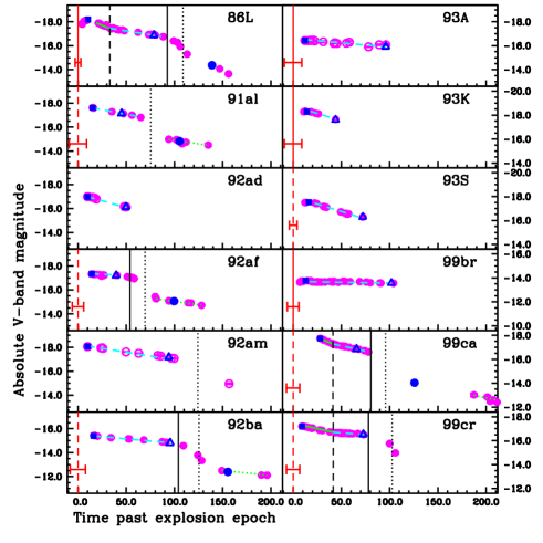
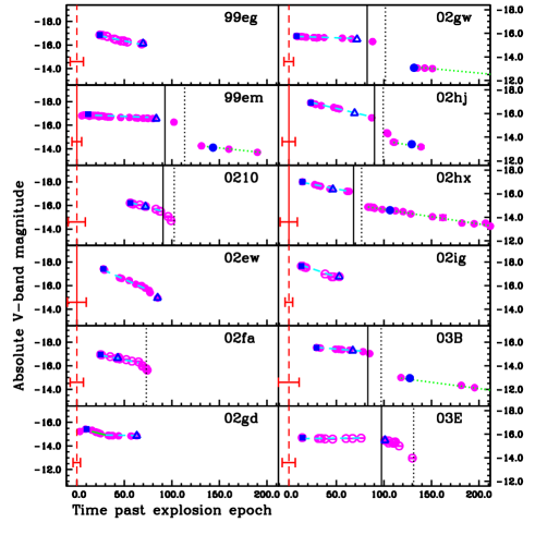
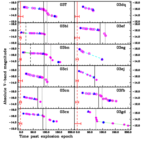
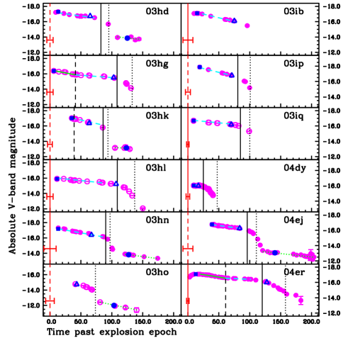
Figure 24.— Absolute magnitude $V$-band light-curves of SNe II in our sample. The panels progress presenting SNe in order of their discovery dates, starting with SN 1986L in the top left panel, and finishing with SN 2004er in the bottom right. Photometry are presented by magenta circles, where open circles indicate that no host galaxy extinction correction was possible (see § 3.3), and hence the presented magnitudes are lower limits. Note that in general errors on the photometry are smaller than the photometric points, and therefore are only visible when they are large in size. Measured light curve parameters are also presented: $M_{\text{max}}$ as blue squares; $M_{\text{end}}$ as blue open triangles; $M_{\text{tail}}$ as blue circles; $s_{1}$ as solid green lines; $s_{2}$ as dashed cyan lines; $s_{3}$ as dotted green lines; $t_{end}$ as solid vertical black lines; $t_{PT}$ as dotted vertical black lines; and $t_{tran}$ as dashed vertical black lines. Red vertical lines are placed at the explosion epoch (0 on the x-axis), and are presented as solid lines if they are derived through non-detections, and dashed lines if they are derived from spectral matching (see § 3.1 for details). Uncertainties in the explosion epochs are illustrated as red error bars. If this line is missing then an explosion epoch estimate was not possible, and light-curves are presented with an arbitrary offset.

Appendix C Additional figures

In Figs 24, 25 and 26 present $V$-band absolute magnitude light-curves for the full sample of 116 SNe II included in this study, where the measured parameters listed in Table 6 and used in the analysis throughout this work, are also provided in figure form. In Fig. 27 an example of the automated $s_{1}$–$s_{2}$ fitting process is displayed, showing examples of where a simple one slope fit (i.e. $s_{2}$ for SN 2008ag), and a two slope slope fit ($s_{1}$, $s_{2}$ for SN 2004er) are good representations of the photometry.

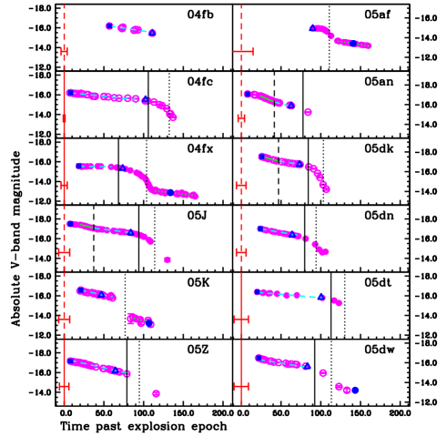
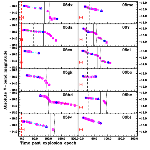
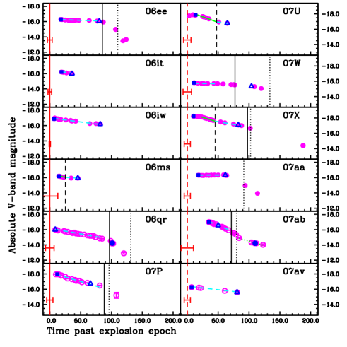
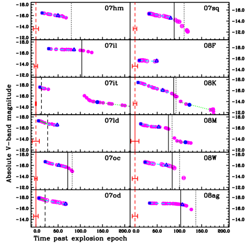
Figure 25.— Absolute magnitude $V$-band light-curves of SNe II in our sample. The panels progress presenting SNe in order of their discovery dates, starting with SN 2004fb in the top left panel, and finishing with SN 2008ag in the bottom right. Presentation of light-curves and their derived parameters takes the same form as in Fig. 24.

In Fig. 28 the correlation between $s_{1}$ and $s_{3}$ is shown. In Fig. 29 we present correlations between the 3 brightness measurements: $M_{\text{max}}$, $M_{\text{end}}$, and $M_{\text{tail}}$. A large degree of correlation between all three is observed. $M_{\text{end}}$ is plotted against $s_{1}$ and $s_{3}$ in Fig. 30. $M_{\text{tail}}$ is plotted against $s_{1}$, $s_{2}$ and $s_{3}$ in Fig. 31. In Fig. 32 we present correlations of $Pd$ and $OPTd$ against $M_{\text{end}}$.

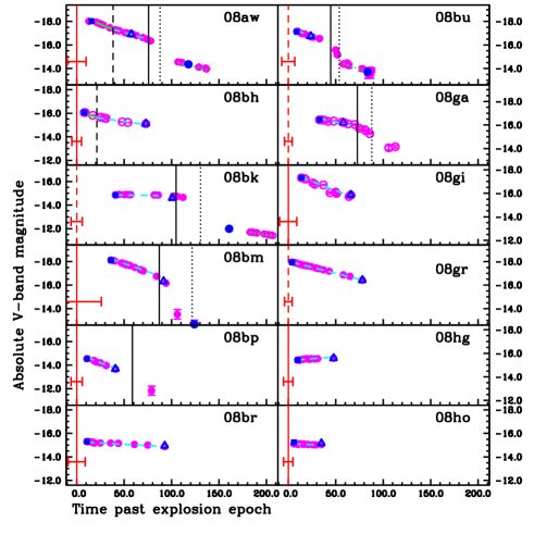
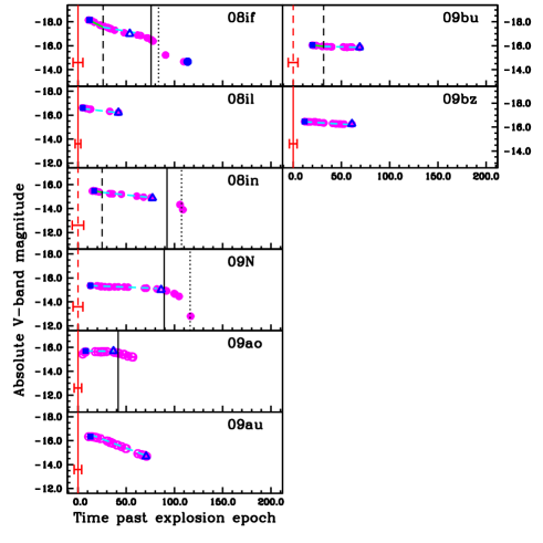
Figure 26.— Absolute magnitude $V$-band light-curves of SNe II in our sample. The panels progress presenting SNe in order of their discovery dates, starting with SN 2008aw in the top left panel, and finishing with SN 2009bz in the bottom right. Presentation of light-curves and their derived parameters takes the same form as in Fig. 24.

In Fig. 33 $M_{\text{end}}$, $M_{\text{max}}$, and $s_{2}$ are plotted against estimated ⁵⁶Ni masses: there appears to be a trend that more luminous SNe synthesize larger amounts of radioactive material, as previously observed by Hamuy (2003a), Bersten (2013) and Spiro et al. (2014), while there is no correlation between ⁵⁶Ni mass and decline rate. Finally, in Fig. 34 $M_{\text{end}}$ and ⁵⁶Ni mass are plotted against the steepness parameter S (see Elmhamdi et al. 2003 for more discussion on this topic), where we do not observe trends seen by previous authors.

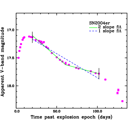
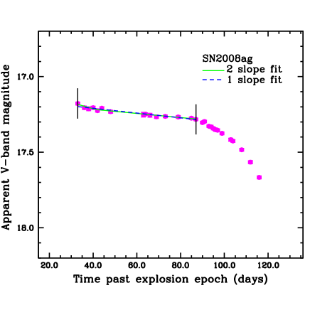
Figure 27.— Examples of the 2-slope fitting process outlined in § 3. Left: fits to the $V$-band photometry for SN 2004er. Here it is clearly observed that the 2-slope model more accurately represents the data. Right: fits to the $V$-band photometry for SN2008ag. In this second case the 1-slope model is just as good as the 2 slope model, therefore adding an extra parameter (the second slope) does not improve the fit.

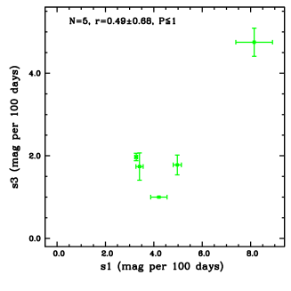
Figure 28.— $s_{1}$ plotted against $s_{3}$.

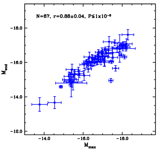
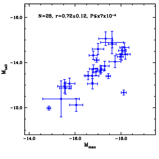
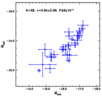
Figure 29.— Correlations between the three measured absolute magnitudes: $M_{\text{max}}$, $M_{\text{end}}$ and $M_{\text{tail}}$. Left: $M_{\text{max}}$ vs. $M_{\text{end}}$. Middle: $M_{\text{max}}$ vs. $M_{\text{tail}}$. Right: $M_{\text{end}}$ vs. $M_{\text{tail}}$. Magnitudes at the three distinct epochs are strongly correlated.

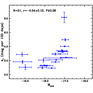
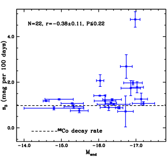
Figure 30.— Left: The magnitude at the end of the ‘plateau’, $M_{\text{end}}$, plotted against the initial decline rate from maximum, $s_{1}$. Right: $M_{\text{end}}$ plotted against the decline rate of the radioactive tail, $s_{3}$. The dashed horizontal line shows the expected decline rate on the radioactive tail, assuming full trapping of gamma-rays from ⁵⁶Co decay.

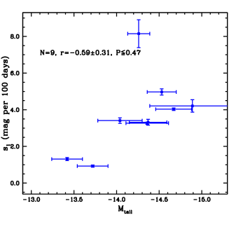
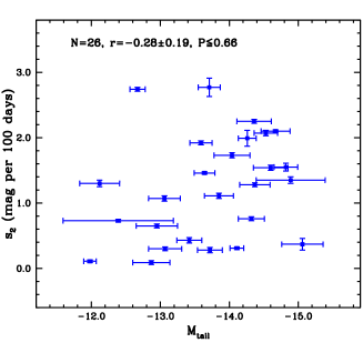
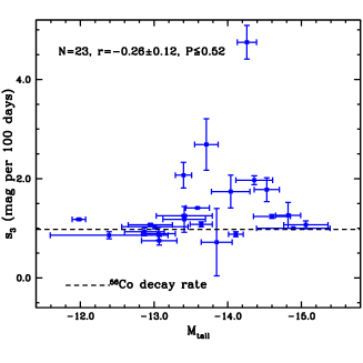
Figure 31.— Left: The magnitude at the beginning of the tail; $M_{\text{tail}}$, plotted against the initial decline rate from maximum; $s_{1}$. Middle: $M_{\text{tail}}$ plotted against the decline rate on the ‘plateau’; $s_{2}$. Right: $M_{\text{tail}}$ plotted against the decline rate of the radioactive tail.

Figure 32.— Left: ‘Plateau’ durations, $Pd$ against $M_{\text{end}}$. Right: SNe optically thick durations, $OPTd$, against $M_{\text{end}}$.

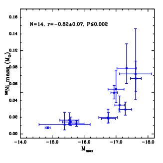
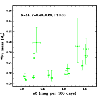
Figure 33.— Left: $M_{\text{end}}$ against ⁵⁶Ni mass. Middle: $M_{\text{max}}$ plotted against ⁵⁶Ni mass. Right: $s_{2}$ against ⁵⁶Ni mass.

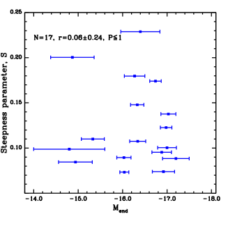
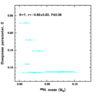
Figure 34.— Left: $M_{\text{end}}$ against ‘steepness’ parameter. Right: ⁵⁶Ni mass against ‘steepness’ parameter.

Table 5SN II $V$-band light-curve parameters.

SN	DM	Explosion	$t_{PT}$	$A_{\rm V}$(Host)	$M_{\text{max}}$	$M_{\text{end}}$	$M_{\text{tail}}$	$s_{1}$	$s_{2}$	$s_{3}$	$OPTd$	$Pd$	56Ni mass
	(mag)	epoch (MJD)	(MJD)	(mag)	(mag)	(mag)	(mag)	(mag 100d-1)	(mag 100d-1)	(mag 100d-1)	(days)	(days)	(${\rm\ M}_{\odot}$)
1986L	31.721(0.20)	46708.0n(6)	46818.4(0.6)	0.00(0.07)	–18.19(0.21)	–16.88(0.22)	–14.37(0.22)	3.32(0.16)	1.28(0.03)	$\cdots$	93.7(5)	59.2(4)	$>$0.061
1991al	33.94(0.15)	48443.5s(9)	48518.8(0.6)	0.11(0.07)	–17.62(0.17)	–17.14(0.17)	–14.82(0.17)	$\cdots$	1.55(0.06)	1.26(0.26)	$\cdots$	$\cdots$	0.067${}^{+0.016}_{-0.021}$
1992ad	31.13(0.80)	$\cdots$	$\cdots$	$\cdots$	–16.98∗(0.80)	–16.13∗(0.80)	$\cdots$	$\cdots$	2.23(0.04)	$\cdots$	$\cdots$	$\cdots$	$\cdots$
1992af	34.33(0.12)	48791.5s(6)	48861.1(0.4)	0.00(0.27)	–17.33(0.30)	–17.20(0.30)	–15.06(0.30)	$\cdots$	0.37(0.09)	1.07(0.08)	54.0(7)	$\cdots$	0.079${}^{+0.018}_{-0.029}$
1992am	36.42(0.05)	$\cdots$	48947.2(0.6)	$\cdots$	–18.06∗(0.07)	–17.17∗(0.08)	$\cdots$	$\cdots$	1.17(0.02)	$\cdots$	$\cdots$	$\cdots$	$\cdots$
1992ba	30.41(0.80)	48888.5s(8)	49014.0(1.2)	0.05(0.03)	–15.39(0.80)	–14.80(0.80)	–12.39(0.80)	$\cdots$	0.73(0.02)	0.86(0.07)	104.0(9)	$\cdots$	0.011${}^{+0.006}_{-0.015}$
1993A	35.44(0.07)	48995.5n(9)	$\cdots$	$\cdots$	–16.44∗(0.07)	–15.91∗(0.07)	$\cdots$	$\cdots$	0.72(0.03)	$\cdots$	$\cdots$	$\cdots$	$\cdots$
1993K	32.95(0.23)	49065.5n(9)	$\cdots$	0.37(0.19)	–18.29(0.30)	–17.61(0.30)	$\cdots$	$\cdots$	2.46(0.08)	$\cdots$	$\cdots$	$\cdots$	$\cdots$
1993S	35.60(0.07)	49130.5s(4)	$\cdots$	0.00(0.24)	–17.52(0.25)	–16.29(0.26)	$\cdots$	$\cdots$	2.52(0.05)	$\cdots$	$\cdots$	$\cdots$	$\cdots$
1999br	31.19(0.40)	51276.5n(4)	$\cdots$	0.00(0.04)	–13.77(0.40)	–13.56(0.40)	$\cdots$	$\cdots$	0.14(0.02)	$\cdots$	$\cdots$	$\cdots$	$>$0.002
1999ca	33.15(0.21)	51277.5s(7)	51373.2(0.8)	0.26(0.15)	–17.74(0.26)	–16.86(0.26)	–14.04(0.26)	3.41(0.15)	1.73(0.04)	1.74(0.33)	80.5(8)	39.3(4)	$>$0.047
1999cr	34.70(0.10)	51247.5s(7)	51350.2(3.1)	0.30(0.15)	–17.20(0.19)	–16.53(0.19)	$\cdots$	1.80(0.06)	0.58(0.06)	$\cdots$	78.1(8)	41.4(4)	$\cdots$
1999eg	34.75(0.10)	51440.5s(7)	$\cdots$	$\cdots$	–16.86∗(0.10)	–16.12∗(0.10)	$\cdots$	$\cdots$	1.70(0.08)	$\cdots$	$\cdots$	$\cdots$	$\cdots$
1999em	30.372(0.07)	51476.5n(5)	51590.1(0.9)	0.18a(0.06)	–16.94(0.10)	–16.55(0.10)	–14.11(0.10)	$\cdots$	0.31(0.02)	0.88(0.05)	96.0(7)	$\cdots$	0.050${}^{+0.008}_{-0.009}$
0210	36.58(0.04)	52489.5(9)s	52591.9(0.3)	$\cdots$	–16.21∗(0.04)	–15.90∗(0.04)	$\cdots$	$\cdots$	2.21(0.08)	$\cdots$	90.6(10)	$\cdots$	$\cdots$
2002ew	35.38(0.08)	52500.5n(10)	$\cdots$	0.00(0.07)	–17.42(0.11)	–14.95(0.12)	$\cdots$	$\cdots$	3.58(0.06)	$\cdots$	$\cdots$	$\cdots$	$\cdots$
2002fa	36.92(0.04)	52503.5s(7)	$\cdots$	$\cdots$	–16.95∗(0.04)	–16.65∗(0.04)	$\cdots$	$\cdots$	1.58(0.10)	$\cdots$	67.3(8)	$\cdots$	$>$0.066
2002gd	32.50(0.28)	52552.5s(4)	$\cdots$	0.00(0.06)	–15.43(0.29)	–14.85(0.29)	$\cdots$	2.87(0.25)	0.11(0.05)	$\cdots$	$\cdots$	$\cdots$	$\cdots$
2002gw	32.98(0.23)	52559.5s(5)	52661.2(0.8)	0.00(0.05)	–15.76(0.24)	–15.48(0.24)	–13.07(0.24)	$\cdots$	0.30(0.03)	0.75(0.09)	82.3(6)	$\cdots$	0.012${}^{+0.003}_{-0.004}$
2002hj	34.87(0.10)	52562.5n(7)	52661.8(0.8)	0.00(0.11)	–16.91(0.16)	–16.03(0.16)	–13.59(0.16)	$\cdots$	1.92(0.03)	1.41(0.01)	90.2(8)	$\cdots$	$>$0.026
2002hx	35.59(0.07)	52582.5n(9)	52658.9(0.8)	0.00(0.23)	–17.00(0.25)	–16.36(0.25)	–14.60(0.25)	$\cdots$	1.54(0.04)	1.24(0.04)	68.0(10)	$\cdots$	0.053${}^{+0.016}_{-0.023}$
2002ig	37.47(0.03)	52572.5s(4)	$\cdots$	$\cdots$	–17.66∗(0.03)	–16.76∗(0.03)	$\cdots$	$\cdots$	2.73(0.11)	$\cdots$	$\cdots$	$\cdots$	$\cdots$
2003B	31.11(0.28)	52616.5s(11)	52713.8(0.9)	0.18(0.09)	–15.54(0.30)	–15.29(0.30)	–12.95(0.30)	$\cdots$	0.65(0.03)	1.07(0.03)	83.2(12)	$\cdots$	0.017${}^{+0.006}_{-0.009}$
2003E	33.92(0.15)	52634.5s(7)	52765.7(0.8)	$\cdots$	–15.70∗(0.15)	–15.48∗(0.15)	$\cdots$	$\cdots$	–0.07(0.03)	$\cdots$	97.4(8)	$\cdots$	$\cdots$
2003T	35.37(0.08)	52654.5n(10)	52758.7(0.6)	$\cdots$	–16.54∗(0.08)	–16.03∗(0.08)	–13.67∗(0.08)	$\cdots$	0.82(0.02)	2.02(0.14)	90.6(11)	$\cdots$	$>$0.030
2003bl	34.02(0.14)	52699.5s(3)	52804.5(0.2)	0.00(0.27)	–15.35(0.31)	–15.01(0.31)	$\cdots$	1.05(0.35)	0.24(0.04)	$\cdots$	92.8(5)	71.7(9)	$\cdots$
2003bn	33.79(0.16)	52694.5n(3)	52813.7(0.7)	0.00(0.07)	–16.80(0.18)	–16.34(0.18)	–13.72(0.18)	0.93(0.06)	0.28(0.04)	$\cdots$	93.0(5)	53.9(5)	$>$0.038
2003ci	35.56(0.07)	52711.5n(8)	52817.7(1.0)	$\cdots$	–16.83∗(0.07)	–15.70∗(0.07)	$\cdots$	$\cdots$	1.79(0.04)	$\cdots$	92.5(9)	$\cdots$	$\cdots$
2003cn	34.48(0.11)	52719.5s(4)	52804.2(0.3)	0.00(0.12)	–16.26(0.17)	–15.61(0.17)	$\cdots$	$\cdots$	1.43(0.04)	$\cdots$	67.8(6)	$\cdots$	$\cdots$
2003cx	35.96(0.06)	52728.5s(5)	52828.5(0.8)	0.00(0.17)	–16.79(0.18)	–16.38(0.19)	–14.32(0.19)	$\cdots$	0.76(0.03)	$\cdots$	87.8(7)	$\cdots$	$>$0.051
2003dq	36.44(0.06)	52731.5n(8)	$\cdots$	$\cdots$	–16.69∗(0.06)	–15.69∗(0.36)	$\cdots$	$\cdots$	2.50(0.19)	$\cdots$	$\cdots$	$\cdots$	$\cdots$
2003ef	34.08(0.14)	52759.5s(9)	52869.9(0.6)	$\cdots$	–16.72∗(0.14)	–16.15∗(0.14)	$\cdots$	$\cdots$	0.81(0.02)	$\cdots$	90.9(10)	$\cdots$	$\cdots$
2003eg	34.23(0.13)	52773.5s(5)	$\cdots$	$\cdots$	–17.81∗(0.13)	–14.57∗(0.13)	$\cdots$	$\cdots$	2.93(0.04)	$\cdots$	$\cdots$	$\cdots$	$\cdots$
2003ej	34.36(0.12)	52775.5n(5)	$\cdots$	0.00(0.09)	–17.66(0.16)	–15.66(0.16)	$\cdots$	$\cdots$	3.46(0.05)	$\cdots$	69.0(7)	$\cdots$	$\cdots$
2003fb	34.43(0.12)	52776.5s(6)	52874.4(0.6)	$\cdots$	–15.56∗(0.13)	–15.25∗(0.13)	–13.10∗(0.14)	$\cdots$	0.48(0.06)	1.61(0.39)	84.3(7)	$\cdots$	$>$0.017
2003gd	29.93(0.40)	52767.5s(15)	52840.9(0.2)	0.43b(0.19)	$\cdots$	–16.40(0.44)	–13.01(0.45)	$\cdots$	$\cdots$	1.03(0.04)	$\cdots$	$\cdots$	0.012${}^{+0.006}_{-0.012}$
2003hd	36.00(0.06)	52857.5s(5)	52952.9(1.2)	0.00(0.19)	–17.29(0.20)	–16.72(0.21)	–13.85(0.21)	$\cdots$	1.11(0.04)	0.72(0.68)	82.4(6)	$\cdots$	0.029${}^{+0.007}_{-0.009}$
2003hg	33.65(0.16)	52865.5n(5)	52998.6(1.1)	$\cdots$	–16.38∗(0.16)	–15.50∗(0.16)	$\cdots$	1.60(0.06)	0.59(0.03)	$\cdots$	108.5(7)	67.1(4)	$\cdots$
2003hk	34.77(0.10)	52867.5s(4)	52961.2(1.6)	$\cdots$	–17.02∗(0.10)	–16.36∗(0.10)	–13.14∗(0.10)	$\cdots$	1.85(0.06)	0.40(0.66)	86.0(6)	$\cdots$	$>$0.017
2003hl	32.39(0.30)	52868.5n(5)	53005.4(0.1)	$\cdots$	–15.91∗(0.30)	–15.23∗(0.30)	$\cdots$	$\cdots$	0.74(0.01)	$\cdots$	108.9(7)	$\cdots$	$\cdots$
2003hn	31.15(0.10)	52866.5n(10)	52963.7(0.1)	0.37c(0.10)	–17.11(0.15)	–16.33(0.15)	–13.64(0.15)	$\cdots$	1.46(0.02)	1.08(0.05)	90.1(10)	$\cdots$	0.035${}^{+0.008}_{-0.011}$
2003ho	33.77(0.16)	52847.5s(7)	52920.9(0.1)	$\cdots$	$\cdots$	–14.75∗(0.16)	–12.00∗(0.16)	$\cdots$	$\cdots$	1.69(0.10)	$\cdots$	$\cdots$	$>$0.005
2003ib	34.97(0.09)	52891.5n(8)	$\cdots$	0.00(0.28)	–17.10(0.30)	–16.09(0.30)	$\cdots$	$\cdots$	1.66(0.05)	$\cdots$	$\cdots$	$\cdots$	$\cdots$
2003ip	34.20(0.13)	52896.5s(4)	52997.6(0.1)	0.13(0.08)	–17.88(0.15)	–16.78(0.16)	$\cdots$	$\cdots$	2.01(0.03)	$\cdots$	80.7(6)	$\cdots$	$\cdots$
2003iq	32.39(0.30)	52919.5n(2)	53019.6(0.1)	$\cdots$	–16.69∗(0.30)	–16.18∗(0.30)	$\cdots$	$\cdots$	0.75(0.03)	$\cdots$	84.9(4)	$\cdots$	$\cdots$
2004dy	35.46(0.07)	53241.0n(3)	53289.0(0.5)	$\cdots$	–16.03∗(0.07)	–16.02∗(0.07)	$\cdots$	$\cdots$	0.09(0.14)	$\cdots$	$\cdots$	25.0(5)	$\cdots$

Table 6SN II $V$-band light-curve parameters –Continued.

SN	DM	Explosion	$t_{PT}$	$A_{\rm V}$(Host)	$M_{\text{max}}$	$M_{\text{end}}$	$M_{\text{tail}}$	$s_{1}$	$s_{2}$	$s_{3}$	$OPTd$	$Pd$	56Ni mass
	(mag)	epoch (MJD)	(MJD)	(mag)	(mag)	(mag)	(mag)	(mag 100d-1)	(mag 100d-1)	(mag 100d-1)	(days)	(days)	(${\rm\ M}_{\odot}$)
2004ej	33.10(0.21)	53224.9s(8)	53338.7(0.6)	0.14(0.07)	–16.76(0.22)	–16.27(0.23)	–13.06(0.23)	$\cdots$	1.07(0.04)	0.89(0.13)	96.1(9)	$\cdots$	0.019${}^{+0.005}_{-0.007}$
2004er	33.79(0.16)	53271.8n(2)	53429.6(2.5)	0.34(0.17)	–17.08(0.24)	–16.01(0.24)	$\cdots$	1.28(0.03)	0.40(0.03)	$\cdots$	120.2(6)	59.2(4)	$\cdots$
2004fb	34.54(0.11)	53242.6s(4)	$\cdots$	$\cdots$	–16.19∗(0.11)	–15.46∗(0.11)	$\cdots$	$\cdots$	1.24(0.07)	$\cdots$	$\cdots$	$\cdots$	$\cdots$
2004fc	31.68(0.31)	53293.5n(1)	53425.9(1.0)	$\cdots$	–16.21∗(0.31)	–15.41∗(0.31)	$\cdots$	$\cdots$	0.82(0.02)	$\cdots$	106.06(4)	$\cdots$	$\cdots$
2004fx	32.82(0.24)	53303.5n(4)	53407.3(0.5)	0.00(0.10)	–15.58(0.26)	–15.33(0.26)	–12.87(0.27)	$\cdots$	0.09(0.03)	0.93(0.08)	68.4(6)	$\cdots$	0.014${}^{+0.004}_{-0.006}$
2005J	33.96(0.14)	53382.8s(7)	53496.6(0.7)	0.22(0.30)	–17.50(0.33)	–16.57(0.33)	$\cdots$	2.11(0.07)	0.96(0.02)	$\cdots$	94.0(8)	56.7(4)	$\cdots$
2005K	35.33(0.08)	53369.8s(7)	53446.6(4.3)	$\cdots$	–16.57∗(0.08)	–16.08∗(0.08)	–13.22∗(0.08)	$\cdots$	1.67(0.13)	2.15(0.71)	$\cdots$	$\cdots$	$>$0.016
2005Z	34.61(0.11)	53396.7n(6)	53491.3(1.3)	$\cdots$	–17.17∗(0.11)	–16.17∗(0.11)	$\cdots$	$\cdots$	1.83(0.01)	$\cdots$	78.8(7)	$\cdots$	$\cdots$
2005af	27.75(0.36)	53323.8s(15)	53434.7(0.2)	0.00(0.12)	$\cdots$	–14.99(0.38)	–13.41(0.38)	$\cdots$	$\cdots$	1.25(0.03)	104.0(16)	$\cdots$	0.026${}^{+0.012}_{-0.021}$
2005an	33.43(0.18)	53428.8s(4)	$\cdots$	$\cdots$	–17.07∗(0.18)	–15.89∗(0.18)	$\cdots$	3.34(0.06)	1.89(0.05)	$\cdots$	77.7(6)	36.3(4)	$\cdots$
2005dk	34.01(0.14)	53599.5s(6)	53702.8(0.4)	$\cdots$	–17.52∗(0.14)	–16.74∗(0.14)	$\cdots$	2.26(0.09)	1.18(0.07)	$\cdots$	84.2(7)	37.5(5)	$\cdots$
2005dn	32.83(0.24)	53601.6s(6)	53695.7(0.7)	0.00(0.16)	–17.01(0.29)	–16.38(0.29)	$\cdots$	$\cdots$	1.53(0.02)	$\cdots$	79.8(7)	$\cdots$	$\cdots$
2005dt	35.02(0.09)	53605.6n(9)	53736.1(0.7)	0.00(0.14)	–16.39(0.17)	–15.84(0.17)	$\cdots$	$\cdots$	0.71(0.04)	$\cdots$	112.9(10)	$\cdots$	$\cdots$
2005dw	34.17(0.13)	53603.6n(9)	53717.0(0.9)	$\cdots$	–16.49∗(0.13)	–15.61∗(0.13)	–13.21∗(0.13)	$\cdots$	1.27(0.04)	$\cdots$	92.6(10)	$\cdots$	$>$0.021
2005dx	35.18(0.08)	53615.9s(7)	53719.7(0.8)	0.00(0.28)	–16.05(0.29)	–15.24(0.29)	–12.12(0.29)	$\cdots$	1.30(0.05)	$\cdots$	85.6(8)	$\cdots$	$>$0.007
2005dz	34.32(0.12)	53619.5n(4)	53730.0(0.6)	0.00(0.12)	–16.57(0.17)	–15.97(0.17)	–13.42(0.18)	1.31(0.08)	0.43(0.04)	$\cdots$	81.9(6)	37.6(5)	$>$0.021
2005es	35.87(0.06)	53638.7n(5)	$\cdots$	$\cdots$	–16.98∗(0.06)	–16.32∗(0.06)	$\cdots$	$\cdots$	1.31(0.05)	$\cdots$	$\cdots$	$\cdots$	$\cdots$
2005gk	35.36(0.08)	$\cdots$	53728.5(0.7)	$\cdots$	–16.44∗(0.08)	–15.89∗(0.08)	–13.56∗(0.08)	$\cdots$	1.25(0.07)	$\cdots$	$\cdots$	$\cdots$	$\cdots$
2005hd	35.38(0.08)	$\cdots$	53700.9(0.4)	$\cdots$	$\cdots$	–17.07∗(0.08)	–15.02∗(0.08)	$\cdots$	1.23(0.13)	1.17(0.06)	$\cdots$	$\cdots$	$\cdots$
2005lw	35.22(0.08)	53716.8s(10)	53840.7(1.4)	$\cdots$	–17.07∗(0.08)	–15.47∗(0.08)	$\cdots$	$\cdots$	2.05(0.04)	$\cdots$	107.2(11)	$\cdots$	$\cdots$
2005me	34.76(0.10)	53721.6s(6)	$\cdots$	$\cdots$	–16.83∗(0.10)	–15.51∗(0.10)	$\cdots$	3.06(0.12)	1.70(0.06)	$\cdots$	76.9(7)	43.6(5)	$\cdots$
2006Y	35.73(0.06)	53766.5n(4)	54824.6(0.5)	0.00(0.11)	–17.97(0.13)	–16.98(0.13)	–14.26(0.13)	8.15(0.76)	1.99(0.12)	4.75(0.34)	47.5(6)	26.9(4)	$>$0.034
2006ai	34.01(0.14)	53781.8s(5)	53854.0(0.5)	0.00(0.09)	–18.06(0.17)	–17.03(0.17)	–14.53(0.17)	4.97(0.17)	2.07(0.04)	1.78(0.24)	63.3(7)	38.1(4)	$>$0.050
2006bc	31.97(0.26)	53815.5n(4)	$\cdots$	$\cdots$	–15.18∗(0.26)	–15.07∗(0.26)	$\cdots$	1.47(0.18)	–0.58(0.04)	$\cdots$	$\cdots$	$\cdots$	$\cdots$
2006be	32.44(0.29)	53805.8s(6)	53901.4(0.1)	0.00(0.16)	–16.47(0.33)	–16.08(0.33)	$\cdots$	1.26(0.08)	0.67(0.02)	$\cdots$	72.9(7)	43.5(4)	$\cdots$
2006bl	35.65(0.07)	53823.8s(6)	$\cdots$	$\cdots$	–18.23∗(0.07)	–16.52∗(0.07)	$\cdots$	$\cdots$	2.61(0.02)	$\cdots$	$\cdots$	$\cdots$	$\cdots$
2006ee	33.87(0.15)	53961.9n(4)	54072.1(0.6)	0.00(0.09)	–16.28(0.18)	–16.04(0.18)	$\cdots$	$\cdots$	0.27(0.02)	$\cdots$	85.2(6)	$\cdots$	$\cdots$
2006it	33.88(0.15)	54006.5n(3)	$\cdots$	0.00(0.10)	–16.20(0.18)	–15.97(0.19)	$\cdots$	$\cdots$	1.19(0.13)	$\cdots$	$\cdots$	$\cdots$	$\cdots$
2006iw	35.42(0.07)	54010.7n(1)	$\cdots$	0.00(0.11)	–16.89(0.13)	–16.18(0.14)	$\cdots$	$\cdots$	1.05(0.03)	$\cdots$	$\cdots$	$\cdots$	$\cdots$
2006ms	33.90(0.15)	54034.0n(13)	$\cdots$	0.00(0.19)	–16.18(0.24)	–15.93(0.24)	$\cdots$	2.07(0.30)	0.11(0.48)	$\cdots$	$\cdots$	$\cdots$	$>$0.056
2006qr	34.02(0.14)	54062.8n(7)	54194.1(1.2)	$\cdots$	–15.99∗(0.14)	–14.24∗(0.14)	$\cdots$	$\cdots$	1.46(0.02)	$\cdots$	96.9(8)	$\cdots$	$\cdots$
2007P	36.18(0.05)	54118.7n(5)	54214.7(1.2)	$\cdots$	–17.96∗(0.05)	–16.75∗(0.05)	$\cdots$	$\cdots$	2.36(0.04)	$\cdots$	88.3(7)	$\cdots$	$\cdots$
2007U	35.14(0.08)	54134.6s(6)	$\cdots$	0.00(0.36)	–17.87(0.37)	–16.78(0.37)	$\cdots$	2.94(0.02)	1.18(0.01)	$\cdots$	$\cdots$	$\cdots$	$\cdots$
2007W	33.22(0.20)	54136.8s(7)	54270.8(0.7)	0.00(0.08)	–15.80(0.22)	–15.34(0.22)	$\cdots$	$\cdots$	0.12(0.04)	$\cdots$	77.3(8)	$\cdots$	$\cdots$
2007X	33.11(0.21)	54143.9s(5)	54256.5(0.6)	0.38(0.19)	–18.22(0.29)	–17.08(0.29)	$\cdots$	2.43(0.06)	1.37(0.03)	$\cdots$	97.7(7)	52.6(4)	$\cdots$
2007aa	31.95(0.27)	54135.8s(5)	54227.4(0.3)	0.00(0.07)	–16.32(0.28)	–16.32(0.28)	$\cdots$	$\cdots$	–0.05(0.02)	$\cdots$	$\cdots$	$\cdots$	$\cdots$
2007ab	34.94(0.09)	54123.9s(10)	54204.0(0.9)	$\cdots$	–16.98∗(0.09)	–16.55∗(0.09)	–14.22∗(0.09)	$\cdots$	3.30(0.08)	2.31(0.22)	71.3(11)	$\cdots$	$>$0.040
2007av	32.56(0.22)	54175.8s(5)	$\cdots$	$\cdots$	–16.27∗(0.22)	–15.60∗(0.22)	$\cdots$	$\cdots$	0.97(0.02)	$\cdots$	$\cdots$	$\cdots$	$>$0.015
2007hm	34.98(0.09)	54335.6s(6)	54414.4(1.3)	0.00(0.15)	–16.47(0.18)	–16.00(0.18)	$\cdots$	$\cdots$	1.45(0.04)	$\cdots$	$\cdots$	$\cdots$	$>$0.045
2007il	34.63(0.11)	54349.8n(4)	$\cdots$	0.00(0.11)	–16.78(0.16)	–16.59(0.16)	$\cdots$	$\cdots$	0.31(0.02)	$\cdots$	103.4(5)	$\cdots$	$\cdots$
2007it	30.34(0.50)	54348.5n(1)	$\cdots$	0.06(0.04)	–17.61(0.50)	–14.89(0.50)	$\cdots$	4.21(0.34)	1.35(0.05)	1.00(0.01)	$\cdots$	$\cdots$	0.072${}^{+0.031}_{-0.054}$
2007ld	35.00(0.09)	54377.5s(8)	$\cdots$	0.00(0.14)	–17.30(0.17)	–16.53(0.17)	$\cdots$	2.93(0.15)	1.12(0.16)	$\cdots$	$\cdots$	$\cdots$	$\cdots$
2007oc	31.29(0.15)	54388.5n(3)	54470.2(0.2)	0.00(0.06)	–16.68(0.17)	–16.02(0.17)	$\cdots$	$\cdots$	1.83(0.01)	$\cdots$	71.6(7)	$\cdots$	$\cdots$
2007od	31.91(0.80)	54402.6s(5)	$\cdots$	0.00(0.06)	–17.87(0.80)	–16.81(0.80)	$\cdots$	2.37(0.05)	1.55(0.01)	$\cdots$	$\cdots$	$\cdots$	$\cdots$
2007sq	34.12(0.13)	54421.8s(4)	54532.4(1.4)	$\cdots$	–15.33∗(0.13)	–14.52∗(0.13)	$\cdots$	$\cdots$	1.51(0.05)	$\cdots$	88.3(6)	$\cdots$	$\cdots$
2008F	34.31(0.12)	54470.6s(6)	$\cdots$	$\cdots$	–15.67∗(0.14)	–15.56∗(0.12)	$\cdots$	$\cdots$	0.45(0.10)	$\cdots$	$\cdots$	$\cdots$	$\cdots$
2008K	35.29(0.08)	54477.7s(4)	54570.3(0.8)	0.00(0.05)	–17.45(0.10)	–16.04(0.10)	–13.40(0.11)	$\cdots$	2.72(0.02)	2.07(0.26)	87.1(6)	$\cdots$	$>$0.013

Table 6SN II $V$-band light-curve parameters –Continued

SN	DM	Explosion	$t_{PT}$	$A_{\rm V}$(Host)	$M_{\text{max}}$	$M_{\text{end}}$	$M_{\text{tail}}$	$s_{1}$	$s_{2}$	$s_{3}$	$OPTd$	$Pd$	56Ni mass
	(mag)	epoch (MJD)	(MJD)	(mag)	(mag)	(mag)	(mag)	(mag 100d-1)	(mag 100d-1)	(mag 100d-1)	(days)	(days)	(${\rm\ M}_{\odot}$)
2008M	32.55(0.28)	54471.7n(9)	54555.2(0.4)	0.00(0.07)	–16.75(0.29)	–16.17(0.29)	–13.41(0.29)	$\cdots$	1.14(0.02)	1.18(0.26)	75.3(10)	$\cdots$	0.020${}^{+0.007}_{-0.010}$
2008W	34.59(0.11)	54485.8s(6)	54586.4(0.8)	$\cdots$	–16.60∗(0.11)	–16.05∗(0.11)	$\cdots$	$\cdots$	1.11(0.04)	$\cdots$	83.8(7)	$\cdots$	$\cdots$
2008ag	33.91(0.15)	54479.9s(6)	54616.8(0.5)	0.00(0.11)	–16.96(0.19)	–16.66(0.19)	$\cdots$	$\cdots$	0.16(0.01)	$\cdots$	103.0(7)	$\cdots$	$\cdots$
2008aw	33.36(0.19)	54517.8n(10)	54605.6(0.5)	0.32(0.16)	–18.03(0.25)	–16.92(0.25)	–14.36(0.25)	3.27(0.06)	2.25(0.03)	1.97(0.09)	75.8(11)	37.4(4)	$>$0.050
2008bh	34.02(0.14)	54543.5n(5)	$\cdots$	$\cdots$	–16.06∗(0.14)	–15.11∗(0.14)	$\cdots$	3.00(0.27)	1.20(0.04)	$\cdots$	$\cdots$	$\cdots$	$\cdots$
2008bk	27.682(0.05)	54542.9s(6)	54673.6(1.1)	0.00(0.05)	–14.86(0.08)	–14.59(0.08)	–11.98(0.07)	$\cdots$	0.11(0.02)	1.18(0.02)	104.8(7)	$\cdots$	0.007${}^{+0.001}_{-0.001}$
2008bm	35.66(0.07)	54522.5n(26)	54620.3(0.4)	0.00(0.07)	–18.12(0.11)	–16.32(0.11)	–12.67(0.10)	$\cdots$	2.74(0.03)	$\cdots$	87.0(26)	$\cdots$	$>$0.014
2008bp	33.10(0.21)	54551.7n(6)	$\cdots$	0.54(0.27)	–14.54(0.34)	–13.67(0.35)	$\cdots$	$\cdots$	3.17(0.18)	$\cdots$	58.6(10)	$\cdots$	$\cdots$
2008br	33.30(0.20)	54555.7n(9)	$\cdots$	0.00(0.15)	–15.30(0.25)	–14.94(0.25)	$\cdots$	$\cdots$	0.45(0.02)	$\cdots$	$\cdots$	$\cdots$	$>$0.026
2008bu	34.81(0.10)	54566.8s(7)	54620.5(1.0)	0.00(0.12)	–17.14(0.16)	–16.74(0.16)	–13.71(0.16)	$\cdots$	2.77(0.14)	2.69(0.52)	44.8(7)	$\cdots$	$>$0.020
2008ga	33.99(0.14)	54711.9s(4)	54799.9(0.8)	$\cdots$	–16.45∗(0.14)	–16.20∗(0.14)	$\cdots$	$\cdots$	1.17(0.08)	$\cdots$	72.8(6)	$\cdots$	$\cdots$
2008gi	34.94(0.09)	54742.7n(9)	$\cdots$	$\cdots$	–17.31∗(0.09)	–15.86∗(0.09)	$\cdots$	$\cdots$	3.13(0.08)	$\cdots$	$\cdots$	$\cdots$	$\cdots$
2008gr	34.76(0.10)	54766.6s(4)	$\cdots$	0.00(0.05)	–17.95(0.12)	–16.97(0.12)	$\cdots$	$\cdots$	2.01(0.01)	$\cdots$	$\cdots$	$\cdots$	$\cdots$
2008hg	34.36(0.12)	54779.8n(5)	$\cdots$	0.00(0.28)	–15.43(0.31)	–15.59(0.31)	$\cdots$	$\cdots$	–0.44(0.05)	$\cdots$	$\cdots$	$\cdots$	$\cdots$
2008ho	32.98(0.23)	54792.7n(5)	$\cdots$	0.16(0.08)	–15.27(0.25)	–15.19(0.25)	$\cdots$	$\cdots$	0.30(0.06)	$\cdots$	$\cdots$	$\cdots$	$\cdots$
2008if	33.56(0.17)	54807.8n(5)	54891.5(0.4)	0.21(0.11)	–18.15(0.20)	–17.00(0.21)	–14.67(0.21)	4.03(0.07)	2.10(0.02)	$\cdots$	75.9(7)	49.8(4)	$>$0.063
2008il	34.61(0.11)	54825.6n(3)	$\cdots$	0.00(0.15)	–16.61(0.19)	–16.22(0.19)	$\cdots$	$\cdots$	0.93(0.05)	$\cdots$	$\cdots$	$\cdots$	$\cdots$
2008in	30.38(0.47)	54822.8s(6)	54930.2(0.1)	0.08(0.05)	–15.48(0.47)	–14.87(0.47)	$\cdots$	1.82(0.20)	0.83(0.02)	$\cdots$	92.2(7)	67.2(5)	$\cdots$
2009N	31.49(0.40)	54846.8s(5)	54963.1(0.2)	0.10(0.06)	–15.35(0.41)	–15.00(0.41)	$\cdots$	$\cdots$	0.34(0.01)	$\cdots$	89.5(7)	$\cdots$	$\cdots$
2009ao	33.33(0.20)	54890.7n(4)	$\cdots$	$\cdots$	–15.79∗(0.20)	–15.78∗(0.20)	$\cdots$	$\cdots$	–0.01(0.12)	$\cdots$	41.7(6)	$\cdots$	$\cdots$
2009au	33.16(0.21)	54897.5n(4)	$\cdots$	$\cdots$	–16.34∗(0.21)	–14.69∗(0.21)	$\cdots$	$\cdots$	3.04(0.02)	$\cdots$	$\cdots$	$\cdots$	$\cdots$
2009bu	33.32(0.19)	54907.9s(5)	$\cdots$	0.00(0.10)	–16.05(0.22)	–15.87(0.22)	$\cdots$	0.98(0.16)	0.18(0.04)	$\cdots$	$\cdots$	$\cdots$	$\cdots$
2009bz	33.34(0.19)	54915.8n(4)	$\cdots$	0.00(0.06)	–16.46(0.20)	–16.26(0.20)	$\cdots$	$\cdots$	0.50(0.02)	$\cdots$	$\cdots$	$\cdots$	$\cdots$

• ^∗Absolute magnitudes are lower limits as no host galaxy extinction correction has been appplied.

• ^aTaken from Hamuy et al. (2001).

• ^bTaken from Hendry et al. (2005).

• ^cTaken from Sollerman et al. (2005).

• ¹Estimated using a SN Ia distance.

• ²Estimated using a Cepheid distance.

• ^sExplosion epoch estimation through spectral matching.

• ⁿExplosion epoch estimation from SN non-detection.

Measurements made of our sample of SNe, as defined in Section 3 and outlined in Fig. 1. In the first column we list the SN name. In column 2 the distance modulus employed for each object is presented, followed by explosion epochs in column 3, and $V$-band host-galaxy extinction values in column 4. If an $A_{\rm V}$ estimate has not been possible (see § 3.3) then subsequent magnitudes are presented as lower limits. In columns 5, 6 and 7 we list the absolute magnitudes of $M_{\text{max}}$, $M_{\text{end}}$ and $M_{\text{tail}}$ respectively. These are followed by the decline rates: $s_{1}$, $s_{2}$ and $s_{3}$, in columns 8, 9 and 10 respectively. In column 11 we present the duration $OPTd$ and in column 12 the $Pd$ values are listed. Finally, in column 13 derived ⁵⁶Ni masses (or lower limits) are presented. 1$\sigma$ errors on all parameters are indicated in parenthesis, and are estimated as outlined in the main text. The values within this table are also archived in a file as part of the photometry package available from http://www.sc.eso.org/~janderso/SNII_A14.tar.gz, where we also include further values/measurements used in the process of our analysis.

References

- Anderson et al. (2012) Anderson, J. P., Habergham, S. M., James, P. A., & Hamuy, M. 2012, MNRAS, 424, 1372
- Andrews et al. (2011) Andrews, J. E. et al. 2011, ApJ, 731, 47
- Antilogus et al. (2005) Antilogus, P. et al. 2005, Central Bureau Electronic Telegrams, 263, 1
- Arcavi et al. (2010) Arcavi, I. et al. 2010, ApJ, 721, 777
- Arcavi et al. (2012) Arcavi, I. et al. 2012, ApJ, 756, L30
- Barbon et al. (1999) Barbon, R., Buondí, V., Cappellaro, E., & Turatto, M. 1999, A&AS, 139, 531
- Barbon et al. (1979) Barbon, R., Ciatti, F., & Rosino, L. 1979, A&A, 72, 287
- Barbon et al. (1982) Barbon, R., Ciatti, F., & Rosino, L. 1982, A&A, 116, 35
- Baron et al. (2004) Baron, E., Nugent, P. E., Branch, D., & Hauschildt, P. H. 2004, ApJ, 616, L91
- Baron et al. (2000) Baron, E. et al. 2000, ApJ, 545, 444
- Barth et al. (2008) Barth, A. J., Bentz, M. C., Thornton, C. E., Chornock, R., & Filippenko, A. V. 2008, Central Bureau Electronic Telegrams, 1313, 1
- Bassett et al. (2007) Bassett, B. et al. 2007, Central Bureau Electronic Telegrams, 1098, 1
- Bersten (2013) Bersten, M. C. 2013, ArXiv e-prints
- Bersten et al. (2011) Bersten, M. C., Benvenuto, O., & Hamuy, M. 2011, ApJ, 729, 61
- Bersten & Hamuy (2009) Bersten, M. C. & Hamuy, M. 2009, ApJ, 701, 200
- Bersten et al. (2012) Bersten, M. C. et al. 2012, ApJ, 757, 31
- Blinnikov & Bartunov (1993) Blinnikov, S. I. & Bartunov, O. S. 1993, A&A, 273, 106
- Blondin & Berlind (2008) Blondin, S. & Berlind, P. 2008, Central Bureau Electronic Telegrams, 1209, 1
- Blondin & Calkins (2007a) Blondin, S. & Calkins, M. 2007a, Central Bureau Electronic Telegrams, 1119, 1
- Blondin & Calkins (2007b) Blondin, S. & Calkins, M. 2007b, Central Bureau Electronic Telegrams, 1171, 1
- Blondin et al. (2007a) Blondin, S., Kirshner, R., Challis, P., & Berlind, P. 2007a, Central Bureau Electronic Telegrams, 1062, 2
- Blondin et al. (2007b) Blondin, S., Modjaz, M., Kirshner, R., Challis, P., & Berlind, P. 2007b, Central Bureau Electronic Telegrams, 838, 1
- Blondin et al. (2006) Blondin, S., Modjaz, M., Kirshner, R., Challis, P., & Hernandez, J. 2006, Central Bureau Electronic Telegrams, 480, 1
- Blondin et al. (2007c) Blondin, S., Modjaz, M., Kirshner, R., Challis, P., & Rines, K. 2007c, Central Bureau Electronic Telegrams, 853, 1
- Blondin & Tonry (2007) Blondin, S. & Tonry, J. L. 2007, ApJ, 666, 1024
- Bouchet et al. (1991) Bouchet, P., della Valle, M., & Melnick, J. 1991, IAU Circ., 5312, 2
- Buta (1982) Buta, R. J. 1982, PASP, 94, 578
- Buton et al. (2007) Buton, C. et al. 2007, Central Bureau Electronic Telegrams, 1050, 1
- Cardelli et al. (1989) Cardelli, J. A., Clayton, G. C., & Mathis, J. S. 1989, ApJ, 345, 245
- Challis (2008) Challis, P. 2008, Central Bureau Electronic Telegrams, 1627, 1
- Challis & Berlind (2008) Challis, P. & Berlind, P. 2008, Central Bureau Electronic Telegrams, 1624, 1
- Challis & Berlind (2009a) Challis, P. & Berlind, P. 2009a, Central Bureau Electronic Telegrams, 1749, 1
- Challis & Berlind (2009b) Challis, P. & Berlind, P. 2009b, Central Bureau Electronic Telegrams, 1671, 1
- Chevalier (1976) Chevalier, R. A. 1976, ApJ, 207, 872
- Chornock et al. (2002a) Chornock, R., Jha, S., Filippenko, A. V., & Barris, B. 2002a, IAU Circ., 8008, 2
- Chornock et al. (2002b) Chornock, R., Li, W. D., & Filippenko, A. V. 2002b, IAU Circ., 7964, 2
- Clocchiatti et al. (1996) Clocchiatti, A. et al. 1996, AJ, 111, 1286
- Cohen et al. (2003) Cohen, J., Cohen, P., West, S., & Aiken, L. S. 2003
- Contreras et al. (2007) Contreras, C., Morrell, N., Gonzalez, S., & Lee, K.-G. 2007, Central Bureau Electronic Telegrams, 1068, 1
- Contreras et al. (2010) Contreras, C. et al. 2010, AJ, 139, 519
- Covarrubias & Morrell (2008) Covarrubias, R. & Morrell, N. 2008, Central Bureau Electronic Telegrams, 1349, 1
- D’Andrea et al. (2010) D’Andrea, C. B. et al. 2010, ApJ, 708, 661
- de Vaucouleurs et al. (1981) de Vaucouleurs, G., de Vaucouleurs, A., Buta, R., Ables, H. D., & Hewitt, A. V. 1981, PASP, 93, 36
- della Valle & Bianchini (1992) della Valle, M. & Bianchini, A. 1992, IAU Circ., 5558, 3
- Dennefeld et al. (2008) Dennefeld, M., Agnoletto, I., Harutyunyan, A., et al. 2008, Central Bureau Electronic Telegrams, 1282, 1
- Dessart & Hillier (2005) Dessart, L. & Hillier, D. J. 2005, A&A, 439, 671
- Dessart et al. (2013) Dessart, L., Hillier, D. J., Waldman, R., & Livne, E. 2013, MNRAS, 433, 1745
- Dessart et al. (2008) Dessart, L. et al. 2008, ApJ, 675, 644
- Dessart et al. (2014) Dessart, L. et al. 2014, ArXiv e-prints
- Doggett & Branch (1985) Doggett, J. B. & Branch, D. 1985, AJ, 90, 2303
- Eastman et al. (1996) Eastman, R. G., Schmidt, B. P., & Kirshner, R. 1996, ApJ, 466, 911
- Elias-Rosa et al. (2003) Elias-Rosa, N. et al. 2003, IAU Circ., 8187, 2
- Elias-Rosa et al. (2010) Elias-Rosa, N. et al. 2010, ApJ, 714, L254
- Elias-Rosa et al. (2011) Elias-Rosa, N. et al. 2011, ApJ, 742, 6
- Elmhamdi et al. (2003) Elmhamdi, A., Chugai, N. N., & Danziger, I. J. 2003, A&A, 404, 1077
- Evans & Phillips (1992) Evans, R. & Phillips, M. M. 1992, IAU Circ., 5625, 2
- Falk & Arnett (1977) Falk, S. W. & Arnett, W. D. 1977, ApJS, 33, 515