Transport as a sensitive indicator of quantum criticality

Abstract

We consider bosonic transport through one-dimensional spin systems. Transport is induced by coupling the spin systems to bosonic reservoirs kept at different temperatures. In the limit of weak-coupling between spins and bosons we apply the quantum-optical master equation to calculate the energy transmitted from source to drain reservoirs. At large thermal bias, we find that the current for longitudinal transport becomes independent of the chain length and is also not drastically affected by the presence of disorder. In contrast, at small temperatures, the current scales inversely with the chain length and is further suppressed in presence of disorder. We also find that the critical behaviour of the ground state is mapped to critical behaviour of the current – even in configurations with infinite thermal bias.

I Introduction

Quantum phase transitions are drastic changes of a system’s ground state when an external control parameter is smoothly varied across a critical value sachdev2000 . Typically, they occur in the continuum limit where the considered system becomes infinitely large. Naturally, a critical behavior of the ground state leads to non-analytic behaviour of almost all observables at zero temperature. However, realistic systems cannot be kept at zero temperature nor can they be perfectly isolated from their environments. In such more generalized scenarios involving dissipation, feedback control or external driving, excited states – which may also exhibit critical behaviour cejnar2006a ; caprio2008a ; perez_fernandez2011a ; dietz2013a ; brandes2013a – become relevant.

On the one hand, such modifications may arise as parts of a detecting environment, as is e.g. exemplified by recent advances in cold atom experiments lignier2007a ; baumann2010a ; baumann2011a . On the other hand, there is evidence that additional couplings may give rise to even richer phase diagrams both in case of driving inoue2010a ; lindner2011a ; jiang2011a ; bastidas2012a ; bastidas2012b or dissipation morrison2008a ; dalla_torre2010a ; bhaseen2012a ; kessler2012a ; hoening2012a .

In contrast, here we will explore the scenario of heat transport through spin chains in the weak-coupling limit, for several reasons: First, in this limit, we do not expect the phase diagram to be modified, and the heat current may rather carry signatures of the critical model behaviour lambert2009a ; vogl2012b . Second, we note that the heat transferred between a quantum system and a reservoir may be unambiguously defined in the weak-coupling limit esposito2010a , whereas this becomes an intricate issue on its own beyond campisi2011a . Third, this limit can be conveniently described by master equations of Lindblad type that preserve positivity lindblad1976a and obey detailed balance relations that induce thermalization with the (fixed) reservoir temperature in equilibrium setups lindblad1976a . Fourth, we consider Ising-type spin chains as these can be easily diagonalized. In particular the quantum Ising model in a transverse field has been an attractive candidate of theoretical studies, and several proposals for its experimental implementation with various systems exist friedenauer2008a ; mostame2008a ; zhang2009a ; coldea2010a ; edwards2010a ; kim2011b . Experimental conditions can usually hardly be perfectly controlled, such that we will also consider the impact of disorder on the heat transport.

A non-equilibrium setup may be engineered by connecting the system to reservoirs at different temperature, which induces for two terminals a heat current from source to drain. We note that basic laws of thermodynamics should be respected even in far from equilibrium setups. For example, the heat current should always flow from hot to cold reservoir and the entropy production in the system should be positive. We note that the method we use – the master equation in positivity-preserving secular approximation applied to multiple reservoirs – has all these features.

This paper is organized as follows: In Sec. II we introduce the physical models we consider here in detail. In Sec. III we describe our methods, namely the quantum master equation and the extraction of heat transport characteristics from it. We also discuss how to diagonalize the central spin systems with or without disorder and review the reduced dynamics at low temperatures. We provide heat transport characteristics for perpendicular and longitudinal transport through a closed spin chain in Secs. IV and V, respectively. Results for longitudinal transport through an open spin chain are presented in Sec. VI. We close with a note on Fourier’s law in Sec. VII and conclusions.

II Model

We want to study heat transport between two bosonic reservoirs ($\hbar=1$ throughout)

$$\mathcal{H}_{\rm B}^{S}=\sum_{k}\omega_{k}^{S}b_{kS}^{\dagger}b_{kS}\,,\qquad\mathcal{H}_{\rm B}^{D}=\sum_{k}\omega_{k}^{D}b_{kD}^{\dagger}b_{kD}$$ (1)

with $b_{k\alpha}$ being a bosonic annihilation operator of a particle with frequency $\omega_{k}^{\alpha}$ in either source ($\alpha=S$) or drain ($\alpha=D$). A thermal gradient between the reservoirs is induced by keeping them at separate thermal equilibrium states $\rho_{\alpha}=e^{-\beta_{\alpha}\mathcal{H}_{\rm B}^{\alpha}}/Z_{\alpha}$, where $\beta_{\alpha}$ denotes the inverse temperature of reservoir $\alpha$. Without loss of generality we assume that the temperature of reservoir $S$ is larger than the temperature of reservoir $D$ ($\beta_{S}<\beta_{D}$).

These reservoirs only interact indirectly via the exchange of energy with a spin chain composed of $N$ spins, where we consider systems of the type

$$\mathcal{H}_{\rm S} = \sum_{i=1}^{N}g_{i}\sigma^{x}_{i}+\sum_{i=1}^{N}\left[J^{y}_{i}\sigma^{y}_{i}\sigma^{y}_{i+1}+J^{z}_{i}\sigma^{z}_{i}\sigma^{z}_{i+1}\right]\,.$$ (2)

Here, $\sigma^{\alpha}_{i}$ denotes the Pauli matrix $\sigma^{\alpha}$ acting only on the $i$-th spin and we use the convention $\sigma^{\alpha}_{N+1}\equiv\sigma^{\alpha}_{1}$. The coefficients $g_{i}$ denote the strength of a local external field whereas $J^{y/z}_{i}$ model a ferromagnetic ($J^{y/z}_{i}<0$) or anti-ferromagnetic ($J^{y/z}_{i}>0$) next-neighbor interaction between the spins. Specific cases are the open disordered spin chain ($J^{y}_{N}=J^{z}_{N}=0$), the open YZ model ($J^{y}_{N}=J^{z}_{N}=0$, $g_{i}=g$, $J^{y}_{i<N}=J^{y}$, $J^{z}_{i<N}=J^{z}$), and the closed YZ-model ($g_{i}=g$, $J^{y}_{i}=J^{y}$, $J^{z}_{i}=J^{z}$), which further reduces for $J^{y}=0$ to the Ising chain in a transverse field. These spin chains have the advantage that they can be mapped to non-interacting fermions

$$\mathcal{H}_{\rm S}=\sum_{q}\epsilon_{q}\eta_{q}^{\dagger}\eta_{q}$$ (3)

with fermionic annihilation operators $\eta_{q}$ of quasiparticles with quasienergy $\epsilon_{q}$. Remarkably, this mapping can be performed with an effort that scales at most polynomially in the system size $N$ bunder1999a and – sufficient symmetry provided – can even be performed analytically pfeuty1970a . Despite their simplicity, such spin chains display rich behaviour such as quantum criticality in the continuum limit $N\to\infty$, where the ground state (and associated observables) changes non-analytically as the parameters of the Hamiltonian are varied across a critical point sachdev2000 .

There are many ways of coupling the source and drain reservoirs via spin chains, see Fig. 1.

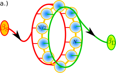
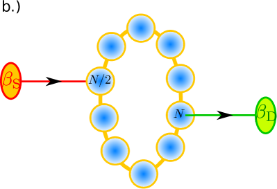
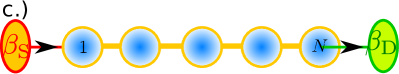
Figure 1: (Color Online) Sketch of heat transport setups considered in this paper. Arrows indicate the energy flow provided a temperature gradient ($\beta_{S}<\beta_{D}$) is present. a.) A homogeneous coupling via $J^{x}=\sum_{i}\sigma^{x}_{i}$ has been considered in vogl2012b . For a homogeneous Ising chain it admits an analytic calculation of the heat current, and the results therein may be readily generalized to the homogeneous YZ-model. b.) In particular for large $N$ it is more reasonable to consider local couplings e.g. via anti-podal points, which we can take as $N/2$ and $N$ via the coupling operator $\sigma^{x}_{N/2}$ and $\sigma^{x}_{N}$, respectively. c.) An open spin chain can be coupled at its ends via the operators $\sigma^{x}_{1}$ and $\sigma^{x}_{N}$ to the bosonic reservoirs.

Our previous study (top panel) revealed that the heat current exhibits features of the critical ground state behaviour even at finite temperatures and large temperature gradients – opposed to local observables such as mean energy or magnetization densities. Here, we would like to learn whether this feature is more generic. More formally, the interaction between system and reservoirs can be written as

$$\mathcal{H}_{\rm SB}=A_{S}\otimes B_{S}+A_{D}\otimes B_{D}\,,$$ (4)

where $A_{\alpha}$ and $B_{\alpha}$ denote system and reservoir operators, respectively. We consider

$$B_{\alpha}=\sum_{k}\left[h_{k\alpha}b_{k\alpha}+h_{k\alpha}^{*}b_{k\alpha}^{\dagger}\right]$$ (5)

throughout this paper, where the $h_{k\alpha}$ ($h_{k\alpha}^{*}$) are the microscopic amplitudes for the annihilation (creation) for a boson of mode $k$ in reservoir $\alpha$. For the system contribution, we had $A_{S}=A_{D}=J^{x}=\sum_{i=1}^{N}\sigma^{x}_{i}$ in Ref. vogl2012b (top panel). Here, we will consider the local couplings $A_{S}=\sigma^{x}_{N/2}$ and $A_{D}=\sigma^{x}_{N}$ (middle panel) for the closed spin chain and $A_{S}=\sigma^{x}_{1}$ and $A_{D}=\sigma^{x}_{N}$ for the open spin chain (bottom panel).

We note that although both $\mathcal{H}_{\rm S}$ and $\mathcal{H}_{\rm B}$ are diagonalizable, the presence of the interaction $\mathcal{H}_{\rm SB}$ requires a perturbative treatment. In contrast, reservoirs consisting of spin chains too would in some cases enable an exact solution arrachea2009a .

III Methods

III.1 Master equation

When the interaction Hamiltonian $\mathcal{H}_{\rm SB}$ is much smaller than the system and reservoir parts, conventional perturbation theory to second order in $h_{k\alpha}$ with standard approximations eventually leads to a closed master equation of Lindblad form lindblad1976a , which in superoperator notation can be written as $\dot{\rho}={\cal L}\rho$. Typically, such a master equation is found valid at high temperatures and/or small coupling strengths. We note that for our model $\left<B_{\alpha}\right>={\rm Tr_{B}}\left\{B_{\alpha}\bar{\rho}_{\alpha}\right\}=0$, which implies that to lowest order both reservoirs enter additively in the master equation ${\cal L}={\cal L}_{S}+{\cal L}_{D}$. In the energy eigenbasis of the system $\mathcal{H}_{\rm S}\left|a\right>=E_{a}\left|a\right>$, the master equation assumes the form

$$\dot{\rho} = -{\rm i}\left[\mathcal{H}_{\rm S}+H_{\rm LS},\rho\right]$$ (6)

$$+\sum_{ab,cd}\gamma_{ab,cd}\left[L_{ab}\rho L_{cd}^{\dagger}-\frac{1}{2}\left\{L_{cd}^{\dagger}L_{ab},\rho\right\}\right]\,,$$

where the Lindblad jumpers $L_{ab}\equiv\left|a\right>\left<b\right|$ trigger transitions between energy eigenstates and where $H_{\rm LS}=\sum_{ab}\tilde{\sigma}_{ab}\left|a\right>\left<b\right|$ denotes the Lamb-shift Hamiltonian. We note here that microscopic derivations in the weak-coupling limit will – a non-trivial system Hamiltonian $\mathcal{H}_{\rm S}$ provided – generally map local terms in the Hamiltonian to non-local Lindblad jumpers. Theories just phenomenologically assuming local Lindblad terms should therefore always be cautiously checked for their thermodynamic consistency saito2003a ; prosen2010a ; sun2010a ; li2011b .

Since the Liouvillian is additively decomposable, this directly transfers to the coefficients $\tilde{\sigma}_{ab}=\tilde{\sigma}_{ab}^{S}+\tilde{\sigma}_{ab}^{D}$ and $\gamma_{ab,cd}=\gamma_{ab,cd}^{S}+\gamma_{ab,cd}^{D}$. Denoting the reservoir-specific interaction by $\mathcal{H}_{\rm SB}^{\alpha}=A_{\alpha}\otimes B_{\alpha}$, these become explicitly breuer2002 ; schaller2008a ; schaller2014

$$\tilde{\sigma}_{ab}^{\alpha} = \frac{\delta_{E_{b},E_{a}}}{2{\rm i}}\sum_{c}\sigma_{\alpha}(E_{a}-E_{c})\left<a\right|A_{\alpha}\left|c\right>\left<c\right|A_{\alpha}\left|b\right>\,,$$

$$\gamma_{ab,cd}^{\alpha} = \delta_{E_{b}-E_{a},E_{d}-E_{c}}\gamma_{\alpha}(E_{b}-E_{a})\left<a\right|A_{\alpha}\left|b\right>\left<c\right|A_{\alpha}\left|d\right>^{*}\,.$$ (7)

Above, we have introduced the even ($\gamma(\omega)$) and odd ($\sigma(\omega)$) Fourier transform of the reservoir correlation function

$$\gamma_{\alpha}(\omega) = \int\left<\mbox{\boldmath$B$}_{\alpha}(\tau)B_{\alpha}\right>e^{+{\rm i}\omega\tau}d\tau\,,$$

$$\sigma_{\alpha}(\omega) = \int\left<\mbox{\boldmath$B$}_{\alpha}(\tau)B_{\alpha}\right>{\rm sgn}(\tau)e^{+{\rm i}\omega\tau}d\tau$$ (8)

$$= \frac{{\rm i}}{\pi}{\cal P}\int\frac{\gamma_{\alpha}(\omega^{\prime})}{\omega-\omega^{\prime}}d\omega^{\prime}\,.$$

We note that we generally have $\left[\mathcal{H}_{\rm S},H_{\rm LS}\right]=0$, which implies that both operators can be simultaneously diagonalized. For the considered bosonic reservoirs the correlation function simply reads schaller2014

$$\gamma_{\alpha}(\omega)=\Gamma_{\alpha}(\omega)\left[1+n_{\alpha}(\omega)\right]$$ (9)

with the Bose distribution $n_{\alpha}(\omega)=\left[e^{\beta_{\alpha}\omega}-1\right]^{-1}$ and the spectral coupling density

$$\Gamma_{\alpha}(\omega)=2\pi\sum_{k}{\left|h_{k\alpha}\right|}^{2}\delta(\omega-\omega_{k\alpha})$$ (10)

that has been analytically continued to negative $\omega$ via $\Gamma_{\alpha}(-\omega)=-\Gamma_{\alpha}(+\omega)$. To obtain analytic results, we parametrize the latter by an ohmic form with a Lorentzian cutoff

$$\Gamma_{\alpha}(\omega)=\Gamma_{\alpha}\frac{\omega}{\Omega}\frac{\delta_{\alpha}^{2}}{\omega^{2}+\delta_{\alpha}^{2}}\,,$$ (11)

where $\Gamma_{\alpha}$ encodes the system-reservoir coupling strength, $\delta_{\alpha}$ the cutoff width, and the energy scale $\Omega$ has just been introduced for dimensional convenience, such that $\Gamma_{\alpha}(\omega)$ has dimension of inverse time ($\hbar=1$ throughout). We note that we expect the master equation description to hold when $\beta_{\alpha}\Gamma_{\alpha}\ll 1$. This parametrization enables one to express the Lamb-shift in closed form as

$$\sigma_{\alpha}(\omega) = -\frac{{\rm i}}{2}\frac{\delta_{\alpha}}{\omega}\Gamma_{\alpha}(\omega)+\frac{{\rm i}}{2}\Gamma_{\alpha}(\omega)\cot\left(\frac{\beta_{\alpha}\delta_{\alpha}}{2}\right)$$

$$-\frac{{\rm i}}{2\pi}\Gamma_{\alpha}(\omega)\left[\Psi\left(1+\frac{\beta_{\alpha}\delta_{\alpha}}{2\pi}\right)+\Psi\left(1-\frac{\beta_{\alpha}\delta_{\alpha}}{2\pi}\right)\right]$$

$$+\frac{{\rm i}}{2\pi}\Gamma_{\alpha}(\omega)\left[\Psi\left(1+{\rm i}\frac{\beta_{\alpha}\omega}{2\pi}\right)+\Psi\left(1-{\rm i}\frac{\beta_{\alpha}\omega}{2\pi}\right)\right]\,,$$

where $\Psi(x)$ denotes the Polygamma (digamma) function abramowitz1970 . We note that $\sigma_{\alpha}(\omega)$ is purely imaginary.

The above quantum-optical master equation has many favorable properties: First, due to its Lindblad form it preserves all density matrix properties, in particular positivity. Second, we note that for the thermal reservoirs considered here the correlation functions satisfy Kubo-Martin-Schwinger (KMS) conditions schaller2014

$$\gamma_{\alpha}(-\omega)=e^{-\beta_{\alpha}\omega}\gamma_{\alpha}(+\omega)\,.$$ (13)

In last consequence, these relations can be used to show that for coupling to a single reservoir, a stationary state of the system is the thermalized one $\rho\propto e^{-\beta\mathcal{H}_{\rm S}}$ with the inverse reservoir temperature $\beta$. Third, it is also easy to see that when the spectrum of $\mathcal{H}_{\rm S}$ is non-degenerate, the populations (diagonals) of the density matrix only couple to themselves

$$\dot{\rho}_{aa}=\sum_{b}\gamma_{ab,ab}\rho_{bb}-\left(\sum_{b}\gamma_{ba,ba}\right)\rho_{aa}$$ (14)

and do thus constitute a rate equation obeying local detailed balance properties. When the spectrum of $\mathcal{H}_{\rm S}$ is partially degenerate, only coherences (off-diagonals) of the density matrix corresponding to degenerate energies will couple to the remaining populations. Depending on the application, the last properties may yield a tremendous reduction of the system dimensionality.

III.2 Heat transport

Consistently, we will consider off-diagonal matrix elements of the density matrix only when they correspond to states that are energetically degenerate, i.e., $\rho_{ij}$ where $E_{i}=E_{j}$. When there are no degeneracies in the spectrum of $\mathcal{H}_{\rm S}$, this implies that the master equation becomes a simple rate equation. The rates $\gamma_{ia,jb}^{\alpha}$ from $\rho_{ab}$ to $\rho_{ij}$ will therefore only be non-vanishing when $E_{a}=E_{b}$ (since $E_{i}=E_{j}$ by construction), and can therefore be associated with the injection or extraction of energy $E_{a}-E_{i}$ from the system due to reservoir $\alpha$. In the long-term limit, the system density matrix will assume a stationary value $\rho\to\bar{\rho}$, and the corresponding energy current into the drain becomes

$$I_{E}=\sum_{ab}\sum_{i}(E_{a}-E_{i})\gamma_{ia,ib}^{D}\bar{\rho}_{ab}\,.$$ (15)

We note here that for a consistent thermodynamic description the energy current between system and reservoir should be defined as above wichterich2007a . The associated particle (matter) current is simply given by

$$I_{M}=\sum_{ab}\sum_{i}\gamma_{ia,ib}^{D}\bar{\rho}_{ab}\,.$$ (16)

To determine the currents, one has to solve the master equation for the stationary state, i.e., in the energy eigenbasis one has to solve the large linear system

$$0 = -{\rm i}(E_{i}-E_{j})\bar{\rho}_{ij}-{\rm i}\sum_{a}(\sigma_{ia}\bar{\rho}_{aj}-\sigma_{aj}\bar{\rho}_{ia})$$ (17)

$$+\sum_{ab}\gamma_{ia,jb}\bar{\rho}_{ab}-\frac{1}{2}(\gamma_{ab,ai}\bar{\rho}_{bj}+\gamma_{aj,ab}\bar{\rho}_{ib})\,.$$

In contrast to our previous setup vogl2012b this has to be done numerically. We note that the associated Liouvillians can become quite large, such that they can no longer be stored in the computer memory as normal matrices. Fortunately, the Liouvillians are also quite sparse, and by storing them in a sparse format simple methods such as power iteration can be used to determine their stationary state.

We note that although not directly evident from Eq. (15) and (16), the net currents will vanish when e.g. the source is decoupled ($\Gamma_{S}(\omega)\to 0$), which is enforced by the modified solution of the stationary state $\bar{\rho}_{ab}$. The observation that the transition rate from state $a$ to state $i$ obeys $\gamma_{ia,ia}^{\alpha}\propto\Gamma_{\alpha}(E_{a}-E_{i})[1+n_{\alpha}(E_{a}-E_{i})]$ leads to a simple interpretation of the transition energies of the system, see Fig. 2.

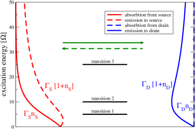
Figure 2: (Color Online) Comparison of emission and absorption rates of source (left, red) and drain (right, blue) with the transition frequencies of the system (center, black). To support transport from source to drain, both the rates for absorption from the source (solid red) and emission into the drain (solid blue) should be large. For the shown large-bias configuration ($\beta_{S}\Omega=0.1$, $\beta_{D}\Omega=10$) the current from source to drain (solid curves) strongly exceeds the opposite current (dashed curves). For the shown setup, the lowest excitation most strongly contributes to the heat current from source to drain. Other parameters: $\Gamma_{S}=\Gamma_{D}$, $\delta_{\alpha}=10\Omega$.

To enable for energetic transmissions through the system it is necessary that the rates at the corresponding transition frequency $\omega$ are finite both for absorption of energy from the source $\Gamma_{S}(\omega)n_{S}(\omega)$ and for emission to the drain $\Gamma_{D}(\omega)[1+n_{D}(\omega)]$. The situation in Fig. 2 is such that – since the inverse transmission process has much smaller rates – transport is in average directed from source to drain. Furthermore, it is also visible that the third transition hardly contributes to transport. The width of the transport window can be modified by the inverse temperatures $\beta_{\alpha}$ and the widths of the spectral coupling densities $\delta_{\alpha}$.

III.3 Spin chain diagonalization

We will first discuss the analytically treatable homogeneous case ($g_{i}=g$ and $J^{y}_{i}=J^{y}$ and $J^{z}_{i}=J^{z}$) with periodic boundary conditions. Then, we discuss the numerically treatable non-homogeneous case of an open spin chain, where the homogeneous open spin chain appears as a special case.

III.3.1 Diagonalization of the homogeneous periodic YZ model

To diagonalize the YZ model in a transverse field

$$\mathcal{H}_{\rm S} = -g\sum_{i=1}^{N}\sigma^{x}_{i}-J_{y}\sum_{i=1}^{N}\sigma^{y}_{i}\sigma^{y}_{i+1}-J_{z}\sum_{i=1}^{N}\sigma^{z}_{i}\sigma^{z}_{i+1}\,,$$ (18)

we first for convenience introduce rescaled variables

$$g=\Omega(1-s)\,,\quad J_{y}=\Omega s\frac{1-\sigma}{2}\,,\quad J_{z}=\Omega s\frac{1+\sigma}{2}\,,$$ (19)

where the parameter $\Omega$ denotes an energy scale of the system, to which all eigenvalues of the system Hamiltonian are proportional. The other parameters $s$ and $\sigma$ are dimensionless, and we find the quantum phase transition from a paramagnetic phase to the ferromagnetic phases at $s_{\rm crit}=1/2$, the two ferromagnetic phases are separated at $\sigma_{\rm crit}=0$ (anisotropy transition).

To avoid lengthy case distinctions we assume that the length $N$ of the chain is an even number. Inserting the Jordan-Wigner transform jordan1928a (see appendix A), the discrete Fourier transform compatible with antiperiodic boundary conditions (see appendix B) and the standard Bogoliubov transform (see appendix C) one can now – in the subspace of an even number of quasiparticles – map the system Hamiltonian to non-interacting fermions sachdev2000 ; dziarmaga2005a

$$\mathcal{H}_{\rm S}=\sum_{k}\epsilon_{k}\left(\eta_{k}^{\dagger}\eta_{k}-\frac{1}{2}\right)\,,$$ (20)

where the energies read bunder1999a

$$\epsilon_{k} = 2\Omega\Big{[}(1-s)^{2}+s^{2}\left(\frac{1-\sigma}{2}\right)^{2}+s^{2}\left(\frac{1+\sigma}{2}\right)^{2}$$

$$-2s(1-s)\cos\left(\frac{2\pi k}{N}\right)+s^{2}\frac{1-\sigma^{2}}{2}\cos\left(\frac{4\pi k}{N}\right)\Big{]}^{1/2}\,.$$

Here, the quasimomentum $k$ may assume half-integer values

$$k\in\left\{-\frac{N-1}{2},-\frac{N-3}{2},\ldots,+\frac{N-3}{2},+\frac{N-1}{2}\right\}\,.$$ (22)

Closer inspection of the energies in Eq. (III.3.1) yields that $\epsilon_{k}\geq 0$.

First, we note that the quasiparticle energies are symmetric $\epsilon_{+k}=\epsilon_{-k}$, which implies that some excited states of the model are degenerate (e.g. states with in total two quasiparticles with quasimomenta $k_{1}=\pm 1/2$ and $k_{2}=\pm 3/2$).

Second, we also express the coupling operator in terms of the fermions

$$\sigma^{x}_{n} = \mbox{\boldmath$1$}-\frac{2}{N}\sum_{kk^{\prime}}\Big{[}$$

$$+u_{k}^{*}u_{k^{\prime}}\eta_{k}^{\dagger}\eta_{k^{\prime}}e^{-{\rm i}(k-k^{\prime})\frac{2\pi n}{N}}+v_{k}v_{k^{\prime}}^{*}\eta_{k}\eta_{k^{\prime}}^{\dagger}e^{+{\rm i}(k-k^{\prime})\frac{2\pi n}{N}}$$

$$+u_{k}^{*}v_{k^{\prime}}^{*}\eta_{k}^{\dagger}\eta_{k^{\prime}}^{\dagger}e^{-{\rm i}(k+k^{\prime})\frac{2\pi n}{N}}+v_{k}u_{k^{\prime}}\eta_{k}\eta_{k^{\prime}}e^{+{\rm i}(k+k^{\prime})\frac{2\pi n}{N}}\Big{]}$$

where it becomes obvious that these local couplings preserve the subspace of even quasiparticle numbers, as either only pairs of quasiparticles are created/annihilated or the total number of quasiparticles is not changed at all. Later-on, we will be particularly interested in the cases $n=N$ and $n=N/2$. Here, the coefficients $u_{k}$ and $v_{k}$ are given by

$$u_{k} \propto \left[(1-s)-s\cos\left(\frac{2\pi k}{N}\right)+\epsilon_{k}/(2\Omega)\right]$$

$$v_{k} \propto s\sigma\sin\left(\frac{2\pi k}{N}\right)$$ (24)

with the normalization condition ${\left|u_{k}\right|}^{2}+{\left|v_{k}\right|}^{2}=1$. Since $\epsilon_{k}\geq 0$ this implies that these coefficients can be chosen real.

Another particularly simple case arises for the coupling $J^{x}=\sum_{i}\sigma^{x}_{i}$, where we can collapse the summation

$$J^{x} = N\mbox{\boldmath$1$}-2\sum_{k}\Big{[}{\left|u_{k}\right|}^{2}\eta_{k}^{\dagger}\eta_{k}+{\left|v_{k}\right|}^{2}\eta_{k}\eta_{k}^{\dagger}$$ (25)

$$-u_{k}^{*}v_{k}^{*}\eta_{+k}^{\dagger}\eta_{-k}^{\dagger}-u_{k}v_{k}\eta_{-k}\eta_{+k}\Big{]}\,,$$

which formally coincides with our previous finding vogl2012b but now also includes the phase parameter $\sigma$ in the coefficients $u_{k}$, $v_{k}$, and $\epsilon_{k}$.

We note here that it is straightforward to represent the system energy density $\left<E\right>/N$ at finite temperature in the continuum limit $N\to\infty$. Using that for a thermal state $\left<E\right>=-\partial_{\beta}\ln Z_{\beta}$ with the partition function $Z_{\beta}={\rm Tr}\left\{e^{-\beta\mathcal{H}_{\rm S}}\right\}$ with Hamiltonian (20) one arrives at the expression

$$\frac{\left<E\right>}{N}\to-\int\limits_{0}^{1/2}\epsilon(\kappa)\tanh\left[\frac{\beta\epsilon(\kappa)}{2}\right]d\kappa\,,$$ (26)

where $\epsilon(\kappa)=\epsilon_{(\kappa\cdot N)}$, compare Eq. (III.3.1). At zero temperature, this just becomes the ground state energy density which reflects the quantum criticality by a divergent second derivative with respect to the control parameters $s$ and $\sigma$. At finite temperature, critical dependence on these control parameters is no longer found. Furthermore, we stress that the one-dimensional quantum Ising model has no thermal phase transition: The specific heat capacity (per spin, we use $k_{\rm B}=1$)

$$C=\frac{\partial}{\partial T}\left(\frac{\left<E\right>}{N}\right)=\frac{1}{T^{2}}\int\limits_{0}^{1/2}\frac{\epsilon^{2}(\kappa)}{1+\cosh\left[\epsilon(\kappa)/T\right]}d\kappa$$ (27)

for example is an analytic function of temperature $T$.

III.3.2 Diagonalization of the inhomogeneous open YZ model

We consider the open YZ-model in a transverse field as a system

$$\mathcal{H}_{\rm S} = \sum_{i=1}^{N}g_{i}\sigma^{x}_{i}+\sum_{i=1}^{N-1}J^{y}_{i}\sigma^{y}_{i}\sigma^{y}_{i+1}+\sum_{i=1}^{N-1}J^{z}_{i}\sigma^{z}_{i}\sigma^{z}_{i+1}\,,$$ (28)

where we have considered open boundary conditions ($J^{y/z}_{N}=0$).

The Jordan-Wigner-transform (see appendix A) non-locally maps the Pauli spin matrices to fermionic annihilation and creation operators. In particular, the resulting Hamiltonian is quadratic in the fermionic operators, which means that it can be diagonalized with a general Bogoliubov transformation

$$c_{i}=\sum_{j}\left(\alpha_{ij}\eta_{j}+\beta_{ij}\eta_{j}^{\dagger}\right)\,,$$ (29)

with new fermionic annihilation (creation) operators $\eta_{j}$ ($\eta_{j}^{\dagger}$) and complex-valued coefficients $\alpha_{ij}$ and $\beta_{ij}$. Finding the optimal transformation can be mapped to the diagonalization of a $2N\times 2N$ matrix, see appendix D. The advantage of this procedure is that the complexity of obtaining the eigenvalues and eigenvectors is polynomial in the chain length $N$ and not exponential as a naive treatment would suggest. Having solved the eigenvalue problem numerically (using e.g. a standard exact diagonalization routine press1994 ), the Hamiltonian can be represented in terms of the coefficients $\alpha_{ij}$ and $\beta_{ij}$

$$H_{S} = \bar{\epsilon}\mbox{\boldmath$1$}+\sum_{j}\epsilon_{j}\eta_{j}^{\dagger}\eta_{j}\,,$$

$$\bar{\epsilon} = \sum_{i}g_{i}+\sum_{ij}\Big{[}-2g_{i}{\left|\beta_{ij}\right|}^{2}$$

$$+(J_{i}^{y}-J_{i}^{z})(\alpha_{ij}\beta_{i+1,j}+{\rm h.c.})$$

$$+(J_{i}^{y}+J_{i}^{z})(\beta_{ij}\beta_{i+1,j}^{*}+{\rm h.c.})\Big{]}\,,$$

$$\epsilon_{j} = \sum_{i}\Big{[}-2g_{i}{\left|\alpha_{ij}\right|}^{2}+2g_{i}{\left|\beta_{ij}\right|}^{2}$$ (30)

$$+(J_{i}^{y}-J_{i}^{z})(\alpha_{i+1,j}\beta_{ij}-\alpha_{ij}\beta_{i+1,j}+{\rm h.c.})$$

$$+(J_{i}^{y}+J_{i}^{z})(\alpha_{ij}\alpha_{i+1,j}^{*}-\beta_{ij}\beta_{i+1,j}^{*}+{\rm h.c.})\Big{]}\,.$$

Obviously, both the vacuum energy $\bar{\epsilon}$ and the single-particle energies $\epsilon_{j}$ are real. Furthermore, it is possible to choose the vacuum as the ground state and $\epsilon_{j}>0$. Technically, the spectrum of a Hamiltonian with this form can easily be calculated in the Fock space representation: Placing $n_{i}\in\{0,1\}$ quasiparticles in every mode $1\leq i\leq N$, the eigenvectors are given by $\left|\mbox{\boldmath$n$}\right>=\left|n_{1},n_{2},\ldots,n_{N}\right>$, and we have $H\left|\mbox{\boldmath$n$}\right>=\left(\alpha+\sum_{j}\epsilon_{j}n_{j}\right)\left|\mbox{\boldmath$n$}\right>$.

A local coupling is in the fermionic quasiparticle basis represented as

$$\sigma^{x}_{n} = \mbox{\boldmath$1$}-2\sum_{kj}\Big{(}\alpha_{nj}^{*}\alpha_{nk}\eta_{j}^{\dagger}\eta_{k}+\beta_{nj}^{*}\beta_{nk}\eta_{j}\eta_{k}^{\dagger}$$ (31)

$$+\alpha_{nj}^{*}\beta_{nk}\eta_{j}^{\dagger}\eta_{k}^{\dagger}+\beta_{nj}^{*}\alpha_{nk}\eta_{j}\eta_{k}\Big{)}\,,$$

and as before it is visible that only pairs of quasiparticles are created or annihilated. For the open chain we will be naturally interested in the cases $n=1$ and $n=N$.

III.4 Low-Temperature Limit

Provided the ground state and the first excited state in the accessible Hilbert space are non-degenerate and sufficiently far separated from the rest of the spectrum we can at low temperatures $(E_{i}-E_{1})\beta_{\alpha}\gg 1$ simplify the long-term dynamics of the resulting master equation to a $2\times 2$ rate equation containing only the ground and first excited state

$${\cal L} = \sum_{\alpha}\Gamma_{\alpha}^{eg}M_{\alpha}^{eg}\left(\begin{array}[]{cc}-n_{\alpha}^{eg}&1+n_{\alpha}^{eg}\\ n_{\alpha}^{eg}&-1-n_{\alpha}^{eg}\end{array}\right)\,,$$ (34)

where $\Gamma_{\alpha}^{eg}=\Gamma_{\alpha}(E_{1}-E_{0})$ is the bare emission/absorption rate and $n_{\alpha}^{eg}=n_{\alpha}(E_{1}-E_{0})$ the Bose distribution, both evaluated at the energy gap between ground ($g$)and first excited ($e$) state. The matrix element $M_{\alpha}^{eg}={\left|\left<0\right|A_{\alpha}\left|1\right>\right|}^{2}$ describes how efficient the system coupling operators $A_{S/D}$ couple ground and first excited state. The matter current then reduces to

$$I_{M} = \frac{\Gamma_{S}^{eg}\Gamma_{D}^{eg}M_{S}^{eg}M_{D}^{eg}}{\Gamma_{S}^{eg}M_{S}^{eg}\left(1+2n_{S}^{eg}\right)+\Gamma_{D}^{eg}M_{D}^{eg}\left(1+2n_{D}^{eg}\right)}\times$$ (35)

$$\times\left(n_{S}^{eg}-n_{D}^{eg}\right)\,,$$

whereas the energy current is tightly coupled to the matter current $I_{E}=(E_{1}-E_{0})I_{M}$. When we neglect the effect of asymmetric source-drain couplings $\Gamma_{S}^{eg}=\Gamma_{D}^{eg}=\Gamma$ and in addition consistently expand the current for low-temperatures, it further reduces to

$$I_{M} \to \Gamma\frac{M_{S}^{eg}M_{D}^{eg}}{M_{S}^{eg}+M_{D}^{eg}}\left(n_{S}^{eg}-n_{D}^{eg}\right)$$ (36)

$$\equiv \Gamma M^{eg}\left(n_{S}^{eg}-n_{D}^{eg}\right)\,.$$

Thus, the scaling behaviour depends in the low-temperature limit strongly on the matrix elements $M_{\alpha}^{eg}$, and a first general idea about the dependence of the current on system properties such as the chain length $N$ and disorder strength at low temperatures can be gained from analyzing $M^{eg}$.

III.5 Consistency Checks

Since the involved master equation are high-dimensional, it is essential to check their consistency. We have done this with a variety of tests (in case of numerical tests this is of course limited by numerical accuracy): First of all, positivity was preserved throughout due to the Lindblad type of the used master equations. Second, all currents vanished in equilibrium when $\beta_{S}=\beta_{D}=\beta$. Third, in equilibrium we also found that the stationary density matrix was just given by the thermal state in the accessible Hilbert space. Fourth, for systems that were intrinsically symmetric between source and drain reservoirs (i.e., no disorder present) we found that the current changed sign when $\beta_{S}$ and $\beta_{D}$ were exchanged. Fifth, for selected small-scale rate equation examples we verified the fluctuation theorem for heat exchange saito2007b ; harbola2007a

$$\lim_{t\to\infty}\frac{P_{+E}}{P_{-E}}=e^{(\beta_{D}-\beta_{S})E}\,,$$ (37)

where $P_{+E}$ denotes the probability of an energy transfer $E$ from source to drain. Technically, we verified this by testing the symmetry of the long-term cumulant-generating function

$${\cal C}(-\xi)={\cal C}(+\xi+{\rm i}(\beta_{D}-\beta_{S}))\,,$$ (38)

where $\xi$ denotes an energy counting field such that $P_{E}=\int e^{{\cal C}(\xi)}e^{-{\rm i}E\xi}d\xi$. For rate equations describing energy transport with two terminals and local detailed balance this is to be expected universally andrieux2009a ; campisi2011a . In particular, the exponent in the right-hand side of Eq. (37) will not depend on the microscopic properties of $\mathcal{H}_{\rm S}$. Sixth, for the open spin chain we verified that the stationary current vanished when the ferromagnetic next-neighbor interactions were turned off at any site of the chain – effectively disconnecting source and drain reservoirs. The same was trivially found true when one reservoir was disconnected. Finally, we did of course verify that in the appropriate limits our master equation approached simplified analytic results.

IV Perpendicular heat transport through the closed chain

We consider the setup depicted in Fig. 1 a.) with coupling operators $A_{S}=A_{D}=J^{x}$ and system Hamiltonian (18). A closer look at the fermionic representation of the coupling operator in Eq. (25) reveals that only the subspace of quasiparticle pairs with opposite quasimomenta will participate in the dynamics connected to the ground state. This subspace – of reduced dimension $2^{N/2}$ instead of $2^{N}$ is in general non-degenerate, and if degeneracies occur the corresponding states are not connected by creation or annihilation of quasiparticle pairs. Therefore, in this reduced subspace, a simple rate equation description applies. In general, high-dimensional rate equations cannot be solved analytically. This is particularly true for systems that do not have special structure such as e.g. tri-diagonal form. Here however we have the particular case that source and drain coupling operators of the system are identical. This leads to a special structure of the rate matrix

$${\cal L}=\sum_{\omega}\sum_{\alpha}\Gamma_{\alpha}(\omega){\cal L}_{0}^{\omega}+\Gamma_{\alpha}(\omega)n_{\alpha}(\omega){\cal L}_{1}^{\omega}\,,$$ (39)

where $\omega$ denotes the energy differences of the system, $\alpha\in\{S,D\}$ labels the reservoir with bare emission/absorption rate $\Gamma_{\alpha}(\omega)$ and Bose distribution $n_{\alpha}(\omega)$, and where ${\cal L}_{0/1}^{\omega}$ are superoperators that are independent of the reservoir. Local detailed balance now implies that one has for all $\omega$ separately

$$\Gamma_{\alpha}(\omega)\left[{\cal L}_{0}^{\omega}+n_{\alpha}(\omega){\cal L}_{1}^{\omega}\right]\bar{\rho}^{\alpha}=0\,,$$ (40)

when $\bar{\rho}^{\alpha}$ is the thermal state, i.e., when

$$\frac{\bar{\rho}^{\alpha}_{n+1}}{\bar{\rho}^{\alpha}_{n}}=\frac{n_{\alpha}(E_{n+1}-E_{n})}{1+n_{\alpha}(E_{n+1}-E_{n})}\,.$$ (41)

The stationary state is thus determined by the function $n_{\alpha}(\omega)$, and by simply rewriting the equation for the total stationary state we obtain

$$0 = \sum_{\omega}\left[\Gamma_{S}(\omega)+\Gamma_{D}(\omega)\right]\times$$ (42)

$$\times\left[{\cal L}_{0}^{\omega}+\frac{\Gamma_{S}(\omega)n_{S}(\omega)+\Gamma_{D}(\omega)n_{D}(\omega)}{\Gamma_{S}(\omega)+\Gamma_{D}(\omega)}{\cal L}_{1}^{\omega}\right]\bar{\rho}\,,$$

such that the stationary state obeys

$$\frac{\bar{\rho}_{n+1}}{\bar{\rho}_{n}}=\frac{\bar{n}(E_{n+1}-E_{n})}{1+\bar{n}(E_{n+1}-E_{n})}$$ (43)

with the average occupation

$$\bar{n}(\omega)=\frac{\Gamma_{S}(\omega)n_{S}(\omega)+\Gamma_{D}(\omega)n_{D}(\omega)}{\Gamma_{S}(\omega)+\Gamma_{D}(\omega)}\,.$$ (44)

We note that resulting stationary state (43) is in general – unless the system has only a single transition frequency vogl2011a – a non-thermal non-equilibrium steady state. This enables the calculation of steady state expectation values such as the current, see below.

IV.1 Finite Thermal Bias

The formal equivalence with our previous results vogl2012b allows us to directly evaluate the stationary energy current

$$I_{E} = \sum_{k>0}\frac{(2\epsilon_{k})(4u_{k}v_{k})^{2}\Gamma_{S}^{k}\Gamma_{D}^{k}(n_{S}^{k}-n_{D}^{k})}{\Gamma_{S}^{k}(1+2n_{S}^{k})+\Gamma_{D}^{k}(1+2n_{D}^{k})}\,,$$ (45)

where we have used the abbreviations $\Gamma_{\alpha}^{k}=\Gamma_{\alpha}(2\epsilon_{k})$ and $n_{\alpha}^{k}=n_{\alpha}(2\epsilon_{k})$. The expression for the matter current simply lacks the $(2\epsilon_{k})$ factor.

Obviously, the current vanishes in equilibrium when $n_{S}(\omega)=n_{D}(\omega)$ as one would reasonably expect. The current is suppressed when either source or drain are decoupled ($\Gamma_{S}^{k}=0$ or $\Gamma_{D}^{k}=0$, respectively). When the coupling strength to source and drain is highly asymmetric, the smaller tunneling rate will bound the current (bottleneck). Therefore, the maximum current can be expected when both reservoirs are about equally coupled but have maximum difference in occupations $n_{S}^{k}\gg n_{D}^{k}$.

Most important however, we find that the current carries the quantum-critical signatures of the ground state somewhat stronger than local observables such as magnetization or energy densities: Whereas the non-analyticities in the continuum limit only occur at strictly zero temperature, the current displays these even far from equilibrium, which we discuss only for the infinite thermal bias limit below.

IV.2 Infinite thermal bias

We will now focus on the infinite thermal bias limit ($n_{S}^{k}\to\infty$ and $n_{D}^{k}\to 0$) with flat spectral coupling densities $\Gamma_{\alpha}^{k}\to\Gamma_{\alpha}$. Provided that the source is not decoupled ($\Gamma_{S}>0$) we see that then the energy current is bounded by the rate to the drain only

$$I_{E}^{\infty} = \Gamma_{D}\sum_{k>0}(2\epsilon_{k})8u_{k}^{2}v_{k}^{2}$$

$$= \sum_{k>0}\frac{8\Gamma_{D}\Omega s^{2}\sigma^{2}\sin^{2}\left(\frac{2\pi k}{N}\right)}{\sqrt{s^{2}\sigma^{2}\sin^{2}\left(\frac{2\pi k}{N}\right)+\left(s+s\cos\left(\frac{2\pi k}{N}\right)-1\right)^{2}}}$$

$$\to \frac{N\Gamma_{D}\Omega}{\pi}4s^{2}\sigma^{2}\times$$

$$\times\int\limits_{0}^{\pi}\frac{\sin^{2}\left(\kappa\right)}{\sqrt{s^{2}\sigma^{2}\sin^{2}\left(\kappa\right)+\left(s+s\cos\left(\kappa\right)-1\right)^{2}}}d\kappa\,,$$

where in the last line we have assumed the continuum limit $N\to\infty$ to convert the summation into an integral. The infinite bias limit leads to the fact that the source tunneling rate has no effect on the current: The system essentially equilibrates with the hot source and is thus always maximally loaded, such that energy transfer to the drain is only limited by $\Gamma_{D}$. Obviously, the current vanishes at the lines defined by $s=0$ and $\sigma=0$: This is consistent with the fact that in these cases we have $\left[J^{x},\mathcal{H}_{\rm S}\right]=0$, such that system and reservoirs cannot exchange energy. Nevertheless, the second derivative of the infinite bias current faithfully detects the quantum-critical behaviour of the ground state also at the critical line $\sigma=0$. To visualize the phase diagram of the model, we therefore plot the norm of the Hessian matrix

$$H\equiv\frac{1}{N\Omega\Gamma_{D}}\left(\begin{array}[]{cc}\partial^{2}_{s}I_{E}^{\infty}&\partial_{s}\partial_{\sigma}I_{E}^{\infty}\\ \partial_{\sigma}\partial_{s}I_{E}^{\infty}&\partial^{2}_{\sigma}I_{E}^{\infty}\end{array}\right)$$ (49)

as a function of the phase parameters $s$ and $\sigma$ in Fig. 3.

\begin{overpic}[clip={true},width=433.62pt]{homog_xy.eps} \put(0.0,55.0){\Large$\sigma$} \put(55.0,0.0){\Large$s$} \end{overpic}

Figure 3: (Color Online) Contour plot of the norm of the Hessian of the energy current (contours represent integer steps in units of $N\Omega\Gamma_{D}$, compare Eq. (49) and Eq. (IV.2)) in the limit of infinite thermal bias versus dimensionless phase parameters $s$ (horizontal axis) and $\sigma$ (vertical axis). The critical lines (white) at $s=1/2$ and $\sigma=0$ are clearly visible as a divergent second derivative, and the current thus faithfully maps the phase diagram of the model. The left sector describes the paramagnetic phase and the top (bottom) right sector the ferromagnetic phase in $z$ ($y$) direction.

It is visible that this norm diverges just at the critical lines of the model defined by $s_{\rm crit}=1/2$ and – in the ferromagnetic phase – by $\sigma_{\rm crit}=0$.

For fixed $\sigma$ or $s$ a closed representation of the current in Eq. (IV.2) in terms of elliptic functions is possible (not shown). Closer inspection of these analytic results reveals that near the critical lines the second derivatives of the current diverge logarithmically – similar to the ground state energy density, e.g.

$$\left.\frac{\partial^{2}I_{E}^{\infty}}{\partial s^{2}}\right|_{\sigma=1} \propto \ln{\left|s-\frac{1}{2}\right|}$$

$$\left.\frac{\partial^{2}I_{E}^{\infty}}{\partial\sigma^{2}}\right|_{s=1} \propto \Theta(\sigma)\ln\sigma\,.$$ (50)

We note that if we had assumed an ohmic spectral coupling density $\Gamma_{\alpha}(\omega)$ as in Eq. (11), the energy current would not display non-analytic behavior. These would then however be persistent in the matter current (which we will analyze in the following models). A super-ohmic choice would result in non-analytic behaviours of the energy current in higher derivatives.

V Longitudinal heat transport along the closed ring

We consider the setup depicted in Fig. 1 b.) with system Hamiltonian (18) and coupling operators $A_{S}=\sigma^{x}_{N/2}$ and $A_{D}=\sigma^{x}_{N}$, compare Eq. (III.3.1). This situation is significantly more complicated than the previous case. Nevertheless, it is not necessary to solve the full $2^{N}$-dimensional problem. First, we note that with proper ground state initialization one can constrain the analysis to the subspace of an even number of quasiparticles, since the coupling operators (III.3.1) can only create or annihilate pairs of quasiparticles. This only reduces the dimension to $2^{N-1}$. Unfortunately, even within this subspace many states are degenerate: Due to the symmetry $\epsilon_{-k}=\epsilon_{+k}$ e.g. states with two quasiparticles with different absolute quasimomenta are four-fold degenerate. For a coupling to a single spin at site $n$, it is possible to show that there exists the conserved quantity

$$Q_{n}=\sum_{q}e^{+{\rm i}4\pi\frac{nq}{N}}\eta_{-q}^{\dagger}\eta_{+q}$$ (51)

obeying $\left[\sigma^{x}_{n},Q_{n}\right]=0$ and $\left[\mathcal{H}_{\rm S},Q_{n}\right]=0$, see Appendix E. Noting that $Q_{n+N/2}=-Q_{n}$ implies that the same quantity is conserved when we consider transport through antipodal points, i.e., $\left[A_{S},Q_{N}\right]=0$ and $\left[A_{D},Q_{N}\right]=0$. The ground state (with no quasiparticles at all) has an associated eigenvalue $Q_{0}=0$, and it therefore suffices to consider only those states that belong to the same subspace as the ground state. Technically, this can be performed by an additional Bogoliubov transformation, see Appendix F. Unfortunately, even in this subspace two-fold degeneracies remain, and the corresponding coherences have to be taken into account, which leads to an overall unfavorable scaling behaviour of the numerical effort with the ring length $N$, summarized in Table 1.

length $N$	dimension $d_{H}$	dimension $d_{L}$	entries $n_{L}$
4	6	8	56
6	20	32	416
8	70	142	2894
10	252	652	19192
12	924	3024	121488
14	3432	14016	738432
16	12870	64614	4331622
18	48620	295724	24629528
20	184756	1343056	136266416

Table 1: Scaling of relevant Hilbert space dimension $d_{H}$, Liouville dimension $d_{L}\times d_{L}$, and the number of non-vanishing entries in the Liouvillian matrix $n_{L}$ with the system size $N$ for longitudinal heat transport through the closed Ising chain. The sparsity of the Liouvillian can be used to calculate its stationary state.

Fortunately, the Liouvillian is sparse, as indicated by its number of non-vanishing entries $n_{L}$, such that sparse matrix techniques have been used for storage and propagation. Furthermore, when one is interested only in e.g. the infinite thermal bias limit, the Liouvillian need not be explicitly stored. In this case, the dimension of the accessible Hilbert space determines the numerical effort: Considering all possible transitions towards a basis state one can use that the coupling allows to create or annihilate only two quasiparticles. With a suitable numerical implementation, this corresponds to two bitflips, such that the numerical effort then only scales roughly as $N^{2}\times d_{H}$.

V.1 Finite temperature configuration

To set up the master equation correctly we introduced an ohmic spectral coupling density (11) and computed also the Lamb-shift terms explicitly. We have not been able to generally solve the master equation analytically for its stationary state. For an ohmic spectral coupling density, we did not find critical dependence of the energy current but for the matter current, which we evaluated numerically for finite problem sizes up to ring lengths of $N=20$ qubits. In finite-sized realizations all divergences are rendered finite, instead of a true divergence one observes a dip, compare Fig. 4.

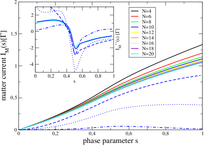
Figure 4: (Color Online) Plot of the matter current through a ring for local couplings at $\sigma=1$ versus phase parameter $s$. At $s=1/2$ the ground state of the system Hamiltonian undergoes the finite-size analog of a second-order quantum phase transition, which manifests itself as a dip in the second derivative (inset). In all curves, the temperature of the drain reservoir was negligible ($\gamma_{D}(\omega)\to\Gamma_{D}(\omega)\Theta(\omega)$). Solid curves correspond to the infinite thermal bias configuration, the other curves (for $N=10$) denote high-bias (dashed, $\beta_{S}\Omega=0.01$), intermediate bias with (dotted, $\beta_{S}\Omega=0.1$), and low-bias (dash-dotted, $\beta_{S}\Omega=1.0$) setups, respectively Other Parameters: $\Gamma_{S}=\Gamma_{D}=\Gamma$, $\delta_{S}=\delta_{D}=1000\Omega$, and $\beta_{D}\Omega\to\infty$.

V.2 Low-temperature configuration

For the closed spin chain with local couplings, the matrix elements of the coupling operators (III.3.1) become independent of the coupling site in the low-temperature limit, such that the average coupling in Eq. (36) becomes

$$M^{eg}={\left|u_{1/2}\right|}^{2}{\left|v_{1/2}\right|}^{2}\frac{2}{N^{2}}\,,$$ (52)

with $u_{1/2}$ and $v_{1/2}$ obeying Eq. (III.3.1). Far from the critical point this scales inversely $I_{M}\propto 1/N^{4}$ with the chain length, and at the critical point one still observes a scaling as $I_{M}\propto 1/N^{2}$ (although here the level separation condition cannot hold for large $N$, since ground state and first excited state approach as $1/N$). An inverse scaling with the chain length might be somewhat expected as the separation between the reservoir increases with $N$. In contrast however, at infinite thermal bias we observe that the current becomes independent of the chain length.

V.3 Infinite thermal bias

In the limit of an infinite thermal bias ($n_{D}(\omega)\to\Theta(\omega)$ and $n_{S}(\omega)\to\infty$) one can however achieve some simplifications. First, we note that the Liouvillian of the source will dominate $\left|\left|L_{S}\right|\right|\gg\left|\left|L_{D}\right|\right|$, such that we can neglect the influence of the drain reservoir on the stationary state. Using further that the source reservoir obeys local detailed balance relations we can conclude that the infinite bias stationary state is the high-temperature state $\rho_{ij}=\delta_{ij}/{\cal N}_{\rm red}$. Here, ${\cal N}_{\rm red}$ is the number of states that participate in the dynamics, i.e., the total number of states with an even number of quasiparticles and with eigenvalue $\lambda_{Q}=0$ for the conserved quantity (51) with $n=N$. Furthermore, the Bose distribution of the drain behaves for low temperatures such that $\gamma_{D}(\omega)=\Gamma_{D}(\omega)\Theta(\omega)$. For large widths $\delta_{D}\to\infty$, this implies that the matter current into the drain becomes

$$I_{M}=\sum_{ia}(E_{a}-E_{i})\Theta(E_{a}-E_{i}){\left|\left<a\right|A_{D}\left|i\right>\right|}^{2}\frac{\Gamma_{D}}{\Omega{\cal N}_{\rm red}}\qquad\,.$$ (53)

Again we note that at infinite thermal bias the drain rate $\Gamma_{D}$ bounds the current. The operator $A_{D}=\sigma^{x}_{N}$ only supports the creation or annihilation of two quasiparticles (which enables one to efficiently evaluate the double summation in the above equation) and thus the difference $E_{a}-E_{i}=\pm\epsilon_{k_{1}}\pm\epsilon_{k_{2}}$ just corresponds to two energies of the quasiparticles.

In case of the Ising model in the ferromagnetic phase ($s=1$ and $\sigma=1$), all excitation energies become similar ($\epsilon_{k}=2\Omega$), and creation of two quasiparticles is the only way for the system to gain energy. Therefore, the expression for the current simplifies in this case to

$$\bar{I}_{M} \to \sum_{ia}\frac{4\Gamma_{D}}{{\cal N}_{\rm red}}\left(\frac{2}{N}\right)^{2}\sum_{kk^{\prime}}{\left|u_{k^{\prime}}\right|}^{2}{\left|v_{k}\right|}^{2}\times$$ (54)

$$\times\left[\cos\left(\frac{\pi}{2}(k+k^{\prime})\right)+\sin\left(\frac{\pi}{2}(k-k^{\prime})\right)\right]^{2}\times$$

$$\times{\left|\left<a\right|\bar{\eta}_{k^{\prime}}^{\dagger}\bar{\eta}_{k}^{\dagger}\left|i\right>\right|}^{2}\,,$$

where we have inserted the additional Bogoliubov transformation relating $\eta_{k}$ and $\bar{\eta}_{k}$, see Appendix F. Further using that $\sum_{i}\left|i\right>\left<i\right|=\mbox{\boldmath$1$}$ we can simplify

$$\bar{I}_{M} \to \frac{4\Gamma_{D}4}{{\cal N}_{\rm red}N^{2}}\sum_{kk^{\prime}}{\left|u_{k^{\prime}}\right|}^{2}{\left|v_{k}\right|}^{2}\times$$ (55)

$$\times\left[\cos\left(\frac{\pi}{2}(k+k^{\prime})\right)+\sin\left(\frac{\pi}{2}(k-k^{\prime})\right)\right]^{2}\times$$

$$\times\sum_{a}\left<a\right|\bar{\eta}_{k}^{\dagger}\bar{\eta}_{k}\bar{\eta}_{k^{\prime}}^{\dagger}\bar{\eta}_{k^{\prime}}\left|a\right>$$

$$= \frac{4\Gamma_{D}}{N^{2}}\left[\sum_{k}{\left|v_{k}\right|}^{2}\left[\cos(\pi k/2)+\sin(\pi k/2)\right]^{2}\right]\times$$

$$\times\left[\sum_{k^{\prime}}{\left|u_{k^{\prime}}\right|}^{2}\left[\cos(\pi k^{\prime}/2)-\sin(\pi k^{\prime}/2)\right]^{2}\right]$$

$$\stackrel{{\scriptstyle N\to\infty}}{{\to}} \Gamma_{D}\,.$$

In the last step, we have performed the continuum limit by replacing the summation over $k$ by analytically solvable integrals. Before, we have used that for very large $N$ one has $\sum_{a}\left<a\right|\bar{\eta}_{k}^{\dagger}\bar{\eta}_{k}\bar{\eta}_{k^{\prime}}^{\dagger}\bar{\eta}_{k^{\prime}}\left|a\right>\approx{\cal N}_{\rm red}/4$, and we can see in Fig. 4 that the actual finite-size current is at $s=1$ only slightly above $\Gamma_{D}$.

Interestingly, we note that the current becomes for large chain lengths independent of $N$. Naively, one might also at infinite bias have expected an inverse scaling of the current $I\propto N^{-\alpha}$ with the ring length, since for large chains the reservoirs are farther apart from each other. Such an inverse scaling is also found in complementary works in the literature benenti2009a ; sun2010a ; znidaric2011a ; li2011a , where local Lindblad operators were assumed (which is applicable in the strong-coupling limit breuer2002 between system and reservoir). However, the above considerations also show that although the matrix elements between two particular states become smaller for longer chains, the mere number of states participating in transport compensates this effect. We expect that this behaviour is only found in the weak-coupling limit, where the pointer basis is given by the energy eigenbasis.

VI Heat transport along the open chain

Here, we investigated the heat current through a homogeneous chain of type (28) that is coupled at its ends to a source reservoir via $A_{S}=\sigma^{x}_{1}$ and a drain reservoir via $A_{D}=\sigma^{x}_{N}$, compare Fig. 1 c.). We exploit that also for an open spin chain or in presence of disorder it is possible to diagonalize the system with only moderate efforts. When the YZ model is opened ($J_{N}^{y}=J_{N}^{z}=0$, we observe that already this removes degeneracies in the energy eigenbasis (these only remain in exceptional points), such that a rate equation description is in principle applicable. We therefore calculated the energy eigenbasis diagonalizing a $2N\times 2N$ auxiliary matrix as described in Appendix. D. Afterwards, we computed the current resulting from the rate equation. The impact of disorder was investigated by distributing the ferromagnetic interaction strengths in $y$-direction uniformly in the interval $J_{i}^{y}\in[\bar{J}^{y}-\Delta J^{y}/2,\bar{J}^{y}+\Delta J^{y}/2]$. We calculated the current for 100 random instances of the spin chain and calculated afterwards mean and variance. Throughout this section, the remaining parameters were chosen as $g_{i}=g=-(1-s)\Omega$ and $J_{i}^{z}=J^{z}=-s\Omega$.

A rate equation representation allows a much simpler numerical implementation of the Liouvillian, since all entries are by construction real. However, since we can only exploit that the number of quasiparticles is always even, the size storage requirements for longitudinal transport along the chain – see Table 2 –

length $N$	dimension $d_{H}$	dimension $d_{L}$	entries $n_{L}$
4	8	8	56
6	32	32	512
8	128	128	3712
10	512	512	23552
12	2048	2048	137216
14	8192	8192	753664
16	32768	32768	3964928
18	131072	131072	20185088
20	524288	524288	100139008

Table 2: Scaling of relevant Hilbert space dimension $d_{H}$, Liouville dimension $d_{L}\times d_{L}$, and the number of non-vanishing entries in the Liouvillian matrix $n_{L}$ with the system size $N$ for longitudinal heat transport along the open chain.

are comparable to the case of longitudinal heat transport through the ring (Table 1). Just as there, sparse matrix methods can be applied to find the stationary state of the Liouvillian. In the limit of an infinite thermal bias however, it is not even necessary to store the full Liouvillian, and the required numerical effort approximately scales as $N^{2}\times d_{H}$.

VI.1 Infinite bias results

Taking a closer look at the representation of the coupling operators in terms of the fermionic quasiparticles (31) we see that we can again constrain the dynamics to the subspace of an even number of quasiparticles. Using the local detailed balance properties of the rates we can conclude that the stationary state in the infinite thermal bias regime will be the equipartitioned distribution of all states with an even number of quasiparticles, such that the infinite bias matter current into the drain is formally identical to Eq. (53). The result is depicted in Fig. 5.

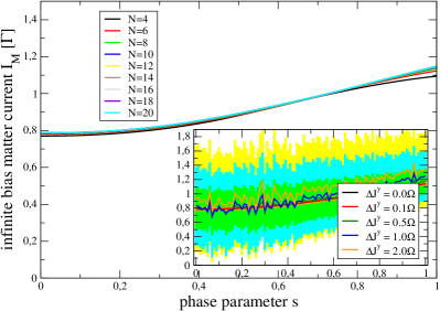
Figure 5: (Color Online) Plot of the phonon current through the open spin chain with homogeneous parameters at infinite thermal bias. Since $J^{y}=\Omega$ is finite throughout, the current does not vanish at $s=0$. The inset demonstrates for $N=10$ that the effect of disorder (solid curves and lighter-shaded areas denote mean and standard deviation obtained from 100 random instances, respectively) at infinite thermal bias is not drastic. Other parameters: $\Gamma_{S}=\Gamma_{D}=\Gamma$, $J^{x}=-(1-s)\Omega$, $J^{z}=-s\Omega$, $J^{y}\in[\Omega-\Delta J^{y}/2,\Omega+\Delta J^{y}/2]$, $\delta_{S}=\Delta_{D}=1000\Omega$.

First, we observe that the infinite bias current is roughly independent of the chain length $N$: Although the matrix element of the coupling operators between two energy eigenstates decreases, the growing number of energy eigenstates compensates this effect. In the inset we demonstrate the effect of increasing the disorder. Somewhat surprisingly, it has little effect on the average current, only the width increases (shaded regions).

VI.2 Low-temperature limit

In the low-temperature limit and assuming level separation of the lowest two states, we investigated the impact of disorder on the current. To do so, we chose the $J_{i}^{y}$ distributed uniformly in the interval $\bar{J}^{y}=[-\Delta J^{y}/2,+\Delta J^{y}/2]$, generated $100$ instances with $g_{i}=-(1-s)\Omega$ and $J_{i}^{z}=J^{z}=-s\Omega$, and calculated the current for each instance in dependence on $s$. For the open spin chain we obtain – adopting the convention that $\epsilon_{a}<\epsilon_{b}<\epsilon_{j\neq\{a,b\}}$ are the smallest two single-particle quasienergies in Eq. (III.3.2) – the expression

$$M_{S}^{eg} = 4\left({\left|\alpha_{1a}\right|}^{2}{\left|\beta_{1b}\right|}^{2}+{\left|\alpha_{1b}\right|}^{2}{\left|\beta_{1a}\right|}^{2}\right)\,,$$

$$M_{D}^{eg} = 4\left({\left|\alpha_{Na}\right|}^{2}{\left|\beta_{Nb}\right|}^{2}+{\left|\alpha_{Nb}\right|}^{2}{\left|\beta_{Na}\right|}^{2}\right)\,,$$ (56)

where $\alpha_{ij}$ and $\beta_{ij}$ are determined by diagonalizing the matrix Eq. (115). Afterwards, we calculated average and variance of the current. As expected, the mean current scales inversely with the system size $N$, see Fig. 6. At the critical point, numerical data suggest a scaling $\propto N^{-2}$ as with the closed chain (compare the crossing point of all curves).

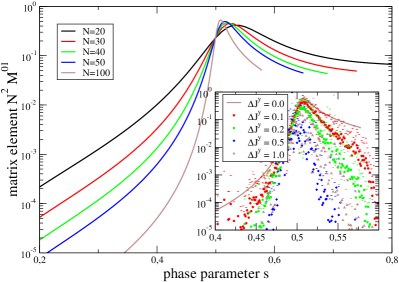
Figure 6: (Color Online) Average coupling matrix element $M^{eg}=M_{S}^{eg}M_{D}^{eg}/(M_{S}^{eg}+M_{D}^{eg})$ constructed from Eq. (VI.2) – scaled by $N^{2}$ – between ground state and first excited state (the energy and matter current at low temperatures are essentially proportional to this coupling matrix element) versus phase parameter $s$. The fact that all curves cross at the critical point is evidence that here the current scales as $\propto N^{-2}$ and decays even faster further away from the critical point. The inset shows the effect of disorder for $N=100$, where quite generally a suppression of the average current (symbols) is observed, especially far from the critical point. Here, thin horizontal lines denote the standard deviation. Other parameters: $J^{x}=-(1-s)\Omega$, $J^{z}=-s\Omega$, $J^{y}\in[-\Delta J^{y}/2,+\Delta J^{y}/2]$ (uniformly distributed).

Furthermore, the inset shows that the presence of disorder further reduces the current, which we interpret as due to the onset of localization of ground state and first excited state, similar to Anderson localization anderson1961a .

VII Scaling versus thermal bias

It is of course possible to combine the different scaling behaviours observed for longitudinal transport at small (inverse with $N$) and large (independent of $N$) thermal biases, see Fig. 7.

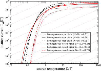
Figure 7: (Color Online) Plot of the phonon matter current versus temperature difference for the closed chain (black curves) and the open chain (red curves) for different regions in the phase space and assuming a vanishing drain temperature. We note that at low source temperature the current scales inversely with the chain length $N$ – with the exponent depending on the phase. At high temperature differences the current reaches a maximum that is independent of $N$. Consistent with our previous results, at low bias the current through critical systems is strongly enhanced in comparison to non-critical system. In contrast, at high bias this is no longer pronounced. Thin straight lines in the background indicate the slope that would be observed if Fourier’s law was obeyed. Other parameters: $\Gamma_{S}=\Gamma_{D}=\Gamma$, $\delta_{S}=\delta_{D}=1000\Omega$, $J^{x}=-(1-s)\Omega$, $J^{y}=0$, $J^{z}=-s\Omega$, and $\beta_{D}\Omega\to\infty$.

It is visible that at low bias, the current strongly decays, and the conductance is surprisingly small. In contrast, at infinite thermal bias the maximum conductance becomes independent on the chain length.

The varying slope of the curves and the fact that the current becomes independent of the temperature difference at large thermal bias indicates that Fourier’s law $I\propto\Delta T$ is not satisfied by the systems considered. We attribute this to the integrability of the models considered saito1996a ; saito2000a ; mejia_monasterio2005a ; manzano2012a ; asadian2013a ; li2011b , which is also not broken if disorder is constrained to the discussed type. Fourier’s law is expected to hold for non-integrable models saito2003a .

VIII Conclusions

We have calculated the heat transport through integrable spin models connected to two bosonic reservoirs kept at different temperatures.

For the closed homogeneous YZ model with homogeneous coupling to the reservoirs we were able to derive an analytic solution for the current. We found that the quantum-critical behaviour of the ground state was faithfully mapped by the current even at extreme bias configurations far from equilibrium. Reasonably, we found for the perpendicular heat transport a linear scaling of the current with the spin chain length.

Complexity was strongly increased when we considered more realistic local couplings to the heat baths. We could exploit the existence of conserved quantities depending on the coupling site to reduce the dimension. In the infinite bias regime we found that the current saturated independent of the chain length, whereas at small temperatures an inverse scaling could be demonstrated. Nevertheless, also in this case our numerical results indicated that the current shows signatures of the critical behaviour.

In the case of an open chain we could – with a simple rate equation approach – reproduce the saturation of the current for large chain lengths and infinite thermal bias. Furthermore, we found that the low-temperature current also shows signatures of the critical point, which remains true when weak disorder is present. Remarkably, we found that disorder did not significantly reduce the average infinite bias current.

None of the systems obeyed Fourier’s law of heat conduction, which we attribute to their integrability. We would also like to emphasize that for a consistent thermodynamic description of transport one should microscopically derive the master equation, since local terms in the interaction Hamiltonian will in general not map to local jump terms in the master equation.

IX Acknowledgements

Financial support by the DFG (SCHA 1646/2-1) is gratefully acknowledged.

Appendix A Jordan-Wigner transform

The Jordan-Wigner-transform is given by

$$\sigma^{x}_{n} = \mbox{\boldmath$1$}-2c_{n}^{\dagger}c_{n}\,,$$

$$\sigma^{y}_{n} = -{\rm i}\left(c_{n}-c_{n}^{\dagger}\right)\prod_{m=1}^{n-1}\left(\mbox{\boldmath$1$}-2c_{m}^{\dagger}c_{m}\right)\,,$$

$$\sigma^{z}_{n} = -\left(c_{n}+c_{n}^{\dagger}\right)\prod_{m=1}^{n-1}\left(\mbox{\boldmath$1$}-2c_{m}^{\dagger}c_{m}\right)\,.$$ (57)

It non-locally maps the Pauli spin matrices to fermionic annihilation and creation operators, where the anti-commutation relations can be easily checked. The inverse of the Jordan-Wigner transform is therefore given by

$$c_{n} = -\frac{1}{2}\left(\sigma^{z}_{n}-{\rm i}\sigma^{y}_{n}\right)\prod_{m=1}^{n-1}\sigma^{x}_{m}\,,$$

$$c_{n}^{\dagger} = -\frac{1}{2}\left(\sigma^{z}_{n}+{\rm i}\sigma^{y}_{n}\right)\prod_{m=1}^{n-1}\sigma^{x}_{m}\,.$$ (58)

Appendix B Discrete Fourier Transform

The discrete Fourier transform

$$c_{n} = \frac{e^{-{\rm i}\pi/4}}{\sqrt{N}}\sum_{k}\tilde{c}_{k}e^{+{\rm i}kn\frac{2\pi}{N}}\,,$$

$$c_{n}^{\dagger} = \frac{e^{+{\rm i}\pi/4}}{\sqrt{N}}\sum_{k}\tilde{c}_{k}^{\dagger}e^{-{\rm i}kn\frac{2\pi}{N}}$$ (59)

maps fermionic operators to new fermionic operators. Its inverse is readily given by

$$\tilde{c}_{k} = \frac{e^{+{\rm i}\pi/4}}{\sqrt{N}}\sum_{n}c_{n}e^{-{\rm i}kn\frac{2\pi}{N}}\,,$$

$$\tilde{c}_{k}^{\dagger} = \frac{e^{-{\rm i}\pi/4}}{\sqrt{N}}\sum_{n}c_{n}^{\dagger}e^{+{\rm i}kn\frac{2\pi}{N}}\,.$$ (60)

In these formulas, the quasimomentum takes the values $k\in\{\pm\frac{1}{2},\pm\frac{3}{2},\ldots,\pm\frac{N-1}{2}\}$, whereas the sites are labeled as $n\in\{1,2,\ldots,N\}$.

Appendix C Homogeneous Bogoliubov Transform

The Bogoliubov transform

$$\tilde{c}_{k} = u_{+k}\eta_{+k}+v_{-k}^{*}\eta_{-k}^{\dagger}\,,$$

$$\tilde{c}_{k}^{\dagger} = u_{+k}^{*}\eta_{+k}^{\dagger}+v_{-k}\eta_{-k}$$ (61)

maps fermions to fermions and preserves the anti-commutation relations when $u_{+k}v_{+k}^{*}+u_{-k}v_{-k}^{*}=0$ and ${\left|u_{+k}\right|}^{2}+{\left|v_{-k}\right|}^{2}=1$. The specific choice of the coefficients

$$u_{k} \propto \left[(1-s)-s\cos\left(\frac{2\pi k}{N}\right)+\epsilon_{k}/(2\Omega)\right]$$

$$v_{k} \propto s\sigma\sin\left(\frac{2\pi k}{N}\right)$$ (62)

with $\epsilon_{k}$ from Eq. (III.3.1) shows that to diagonalize the Hamiltonian, the coefficients can be chosen real. In particular, we have the relations $u_{-k}=+u_{+k}$ and $v_{-k}=-v_{+k}$. Computing the inverse transformation therefore yields

$$\eta_{+k} = u_{-k}^{*}\tilde{c}_{+k}-v_{-k}^{*}\tilde{c}_{-k}^{\dagger}\,,$$

$$\eta_{+k}^{\dagger} = u_{-k}\tilde{c}_{+k}^{\dagger}-v_{-k}\tilde{c}_{-k}\,.$$ (63)

Appendix D Inhomogeneous Bogoliubov Transform

After the Jordan-Wigner transformation, the Hamiltonian (28) reads

$$\mathcal{H}_{\rm S} = \sum_{i=1}^{N}\left[g_{i}\mbox{\boldmath$1$}-2g_{i}c_{i}^{\dagger}c_{i}\right]$$ (64)

$$+\sum_{i=1}^{N}\Big{[}+(J_{i}^{y}-J_{i}^{z})\left(c_{i}c_{i+1}+c_{i+1}^{\dagger}c_{i}^{\dagger}\right)$$

$$+(J_{i}^{y}+J_{i}^{z})\left(c_{i}^{\dagger}c_{i+1}+c_{i+1}^{\dagger}c_{i}\right)\Big{]}\,,$$

i.e., it is a quadratic fermionic Hamiltonian that can be diagonalized with standard methods. To obtain a diagonal (single-particle) representation, where the hopping terms like $c_{i}c_{i+1}^{\dagger}$ and also particle-nonconserving terms like $c_{i}c_{i+1}$ are absent, we introduce the most general Bogoliubov transformation (29). The new operators also obey fermionic anti-commutation relations $\left\{\eta_{i},\eta_{j}^{\dagger}\right\}=\delta_{ij}$ and $\left\{\eta_{i},\eta_{j}\right\}=0$. Preservation of the anti-commutation relations requires for the coefficients

$$0 = \sum_{j}\left(\alpha_{ij}\beta_{i^{\prime}j}+\alpha_{i^{\prime}j}\beta_{ij}\right)\,,$$

$$\delta_{ii^{\prime}} = \sum_{j}\left(\alpha_{ij}\alpha_{i^{\prime}j}^{*}+\beta_{ij}\beta_{i^{\prime}j}^{*}\right)\,,$$ (65)

where ^∗ denotes the complex conjugate. This does not yet fix the transformation. In addition, we demand that the Hamiltonian becomes diagonal in quasiparticle representation

$$H_{S}=\sum_{j}\left[\alpha_{j}\eta_{j}^{\dagger}\eta_{j}+\beta_{j}\eta_{j}\eta_{j}^{\dagger}+\gamma_{j}\mbox{\boldmath$1$}\right]\,.$$ (66)

Inserting the Bogoliubov transformation and setting – after appropriate symmetry transformations – the coefficients of undesired terms to zero yields further constraints, which read explicitly

$$\delta_{jk} \propto \sum_{i}\Big{[}-2g_{i}\alpha_{ij}^{*}\alpha_{ik}+2g_{i}\beta_{ij}\beta_{ik}^{*}$$

$$+(J_{i}^{y}-J_{i}^{z})\times$$

$$\times(\beta_{ij}\alpha_{i+1,k}+\alpha_{i+1,j}^{*}\beta_{ik}^{*}-\beta_{i+1,j}\alpha_{ik}-\alpha_{ij}^{*}\beta_{i+1,k}^{*})$$

$$+(J_{i}^{y}+J_{i}^{z})\times$$

$$\times(\alpha_{ij}^{*}\alpha_{i+1,k}+\alpha_{i+1,j}^{*}\alpha_{ik}-\beta_{i+1,j}\beta_{ik}^{*}-\beta_{ij}\beta_{i+1,k}^{*})\Big{]}$$

$$0 = -2g_{i}\beta_{ij}^{*}\alpha_{ik}+2g_{i}\alpha_{ij}\beta_{ik}^{*}$$

$$+(J_{i}^{y}-J_{i}^{z})\times$$

$$\times(\alpha_{ij}\alpha_{i+1,k}+\beta_{i+1,j}^{*}\beta_{ik}^{*}-\alpha_{i+1,j}\alpha_{ik}-\beta_{ij}^{*}\beta_{i+1,k}^{*})$$

$$+(J_{i}^{y}+J_{i}^{z})\times$$

$$\times(\beta_{ij}^{*}\alpha_{i+1,k}+\beta_{i+1,j}^{*}\alpha_{ik}-\alpha_{i+1,j}\beta_{ik}^{*}-\alpha_{ij}\beta_{i+1,k}^{*})\Big{]}$$

Solving Eqns. (D) and (D) simultaneously can be mapped to solving the eigenvalue problem of a hermitian matrix, such that a solution always exists.

First, by defining the $2N$ vectors

$$\left|V_{k}\right>=\left(\begin{array}[]{c}\left(\begin{array}[]{c}\alpha_{k1}\\ \beta_{k1}\end{array}\right)\\ \vdots\\ \left(\begin{array}[]{c}\alpha_{kN}\\ \beta_{kN}\end{array}\right)\end{array}\right)\,,\qquad\left|\bar{V}_{k}\right>=\left(\begin{array}[]{c}\left(\begin{array}[]{c}\beta_{k1}^{*}\\ \alpha_{k1}^{*}\end{array}\right)\\ \vdots\\ \left(\begin{array}[]{c}\beta_{kN}^{*}\\ \alpha_{kN}^{*}\end{array}\right)\end{array}\right)\,,\qquad$$ (82)

we see that Eqns.(D) can be expressed as the orthonormality conditions $\left<\bar{V}_{k^{\prime}}|\bar{V}_{k}\right>=\delta_{kk^{\prime}}$, $\left<V_{k^{\prime}}|V_{k}\right>=\delta_{kk^{\prime}}$, and $\left<\bar{V}_{k^{\prime}}|V_{k}\right>=0$. Hence, arranging these vectors in a unitary matrix

$${\cal U}=\left(\begin{array}[]{ccc}\left(\begin{array}[]{cc}\alpha_{11}&\beta_{11}^{*}\\ \beta_{11}&\alpha_{11}^{*}\end{array}\right)&\ldots&\left(\begin{array}[]{cc}\alpha_{N1}&\beta_{N1}^{*}\\ \beta_{N1}&\alpha_{N1}^{*}\end{array}\right)\\ \vdots&&\vdots\\ \left(\begin{array}[]{cc}\alpha_{1N}&\beta_{1N}^{*}\\ \beta_{1N}&\alpha_{1N}^{*}\end{array}\right)&\ldots&\left(\begin{array}[]{cc}\alpha_{NN}&\beta_{NN}^{*}\\ \beta_{NN}&\alpha_{NN}^{*}\end{array}\right)\end{array}\right)$$ (94)

we use that the rows are also by construction orthonormal to define the vectors

$$\left|W_{k}\right>=\left(\begin{array}[]{c}\left(\begin{array}[]{c}\alpha_{1k}\\ \beta_{1k}^{*}\end{array}\right)\\ \vdots\\ \left(\begin{array}[]{c}\alpha_{Nk}\\ \beta_{Nk}^{*}\end{array}\right)\end{array}\right)\,,\qquad\left|\bar{W}_{k}\right>=\left(\begin{array}[]{c}\left(\begin{array}[]{c}\beta_{1k}\\ \alpha_{1k}^{*}\end{array}\right)\\ \vdots\\ \left(\begin{array}[]{c}\beta_{Nk}\\ \alpha_{Nk}^{*}\end{array}\right)\end{array}\right)\,.\qquad$$ (109)

Choosing these orthonormal $\left<W_{k}|W_{k^{\prime}}\right>=\delta_{kk^{\prime}}$, $\left<\bar{W}_{k}|\bar{W}_{k^{\prime}}\right>=\delta_{kk^{\prime}}$, and $\left<\bar{W}_{k}|W_{k^{\prime}}\right>=0$ automatically satisfies Eqns. (D).

One can show that Eqns. (D) be written in terms of the vectors $\left|W_{k}\right>$ and $\left|\bar{W}_{k}\right>$ as $\left<W_{j}\right|M\left|W_{k}\right>\propto\delta_{jk}$ or $-\left<{\bar{W}}_{j}\right|M\left|{\bar{W}}_{k}\right>^{*}\propto\delta_{jk}$, respectively, and $\left<\bar{W}_{j}\right|M\left|W_{k}\right>=0$. The matrix $M$ is the $2N\times 2N$-dimensional hermitian and band diagonal matrix

$$M=\left(\begin{array}[]{ccccc}\mbox{\boldmath$D$}_{1}&\mbox{\boldmath$J$}_{1}&\mbox{\boldmath$0$}&\ldots&\mbox{\boldmath$0$}\\ \mbox{\boldmath$J$}_{1}^{\dagger}&\mbox{\boldmath$D$}_{2}&\mbox{\boldmath$J$}_{2}&\ddots&\vdots\\ \mbox{\boldmath$0$}&\mbox{\boldmath$J$}_{2}^{\dagger}&\mbox{\boldmath$D$}_{3}&\mbox{\boldmath$\ddots$}&\mbox{\boldmath$0$}\\ \vdots&\ddots&\ddots&\ddots&\mbox{\boldmath$J$}_{N-1}\\ \mbox{\boldmath$0$}&\ldots&\mbox{\boldmath$0$}&\mbox{\boldmath$J$}_{N-1}^{\dagger}&\mbox{\boldmath$D$}_{N}\end{array}\right)$$ (115)

with the $2\times 2$ matrices

$$\mbox{\boldmath$D$}_{i} = \left(\begin{array}[]{cc}-2g_{i}&0\\ 0&+2g_{i}\end{array}\right)\,,$$ (118)

$$\mbox{\boldmath$J$}_{i} = \left(\begin{array}[]{cc}+(J_{i}^{y}+J_{i}^{z})&-(J_{i}^{y}-J_{i}^{z})\\ +(J_{i}^{y}-J_{i}^{z})&-(J_{i}^{y}+J_{i}^{z})\end{array}\right)\,.$$ (121)

Clearly, Eqns. (D) (and of course orthonormality (D)) are automatically fulfilled when one chooses the $\left|W\right>$ and $\left|\bar{W}\right>$ vectors as eigenvectors of the matrix $M$. The matrix $M$ has a mirror symmetry in its eigenvalues, for each positive eigenvalue $M\left|W_{k}\right>=+\epsilon_{k}\left|W_{k}\right>$ we have also the negative eigenvalue $M\left|\bar{W}_{k}\right>=-\epsilon_{k}\left|\bar{W}_{k}\right>$.

Appendix E Conserved Quantities for local couplings

The system Hamiltonian has many degenerate levels (e.g. those where the total quasimomentum does not vanish). This is due to the fact that only the absolute value of the quasimomentum $k$ enters the energy. One can easily show that an operator of the form $Q=\sum_{q}f_{q}\eta_{-q}^{\dagger}\eta_{+q}$ where hermiticity requires $f_{-q}^{*}=f_{+q}$, will commute with the system Hamiltonian. Therefore, we use this as an ansatz to find a conserved quantity under local couplings. To reduce the computational effort we first rewrite the coupling operator (III.3.1) as

$$\sigma^{x}_{n} = \left[1-\frac{2}{N}\sum_{k}{\left|v_{k}\right|}^{2}\right]\mbox{\boldmath$1$}$$ (122)

$$-\frac{2}{N}\sum_{kk^{\prime}}\left(u_{k}^{*}u_{k^{\prime}}-v_{k}^{*}v_{k^{\prime}}\right)e^{-{\rm i}(k-k^{\prime})\frac{2\pi n}{N}}\eta_{k}^{\dagger}\eta_{k^{\prime}}$$

$$-\frac{2}{N}\sum_{kk^{\prime}}\left(v_{k}u_{k^{\prime}}e^{+{\rm i}(k+k^{\prime})\frac{2\pi n}{N}}\eta_{k}\eta_{k^{\prime}}+{\rm h.c.}\right)\,,$$

where the terms in the second row conserve the total quasiparticle number and the terms in the last row do not. To obtain a conserved quantity in presence of the reservoir, the commutator of both terms $[Q,\sigma^{x}_{n}]=C_{1}+C_{2}$ should vanish. The commutator arising from the particle-number conserving terms becomes

$$C_{1} = \sum_{kk^{\prime}q}f_{q}(u_{k}^{*}u_{k^{\prime}}-v_{k}^{*}v_{k^{\prime}})e^{-{\rm i}(k-k^{\prime})\frac{2\pi n}{N}}\left[\eta_{-q}^{\dagger}\eta_{+q},\eta_{+k}^{\dagger}\eta_{+k^{\prime}}\right]$$ (123)

$$= \sum_{q}\left(f_{-q}e^{+{\rm i}\frac{4\pi nq}{N}}-f_{+q}e^{-{\rm i}\frac{4\pi nq}{N}}\right)\eta_{+q}^{\dagger}\eta_{+q}$$

$$+\sum_{q}\sum_{k\neq\pm q}\left(f_{-q}e^{+{\rm i}(q+k)\frac{2\pi n}{N}}-f_{+k}e^{-{\rm i}(q+k)\frac{2\pi n}{N}}\right)\times$$

$$\times(u_{q}^{*}u_{k}+v_{q}^{*}v_{k})\eta_{q}^{\dagger}\eta_{k}$$

$$= \sum_{qk}\left(f_{-q}e^{+{\rm i}(q+k)\frac{2\pi n}{N}}-f_{+k}e^{-{\rm i}(q+k)\frac{2\pi n}{N}}\right)\times$$

$$\times(u_{q}^{*}u_{k}+v_{q}^{*}v_{k})\eta_{q}^{\dagger}\eta_{k}\,.$$

The second commutator becomes

$$C_{2} = \sum_{kk^{\prime}q}f_{q}v_{k}u_{k^{\prime}}e^{+{\rm i}(k+k^{\prime})\frac{2\pi n}{N}}\left[\eta_{-q}^{\dagger}\eta_{+q},\eta_{+k}\eta_{+k^{\prime}}\right]$$ (124)

$$= \sum_{q}\sum_{k\neq\pm q}\left(-f_{q}e^{+{\rm i}(k-q)\frac{2\pi n}{N}}+f_{k}e^{-{\rm i}(k-q)\frac{2\pi n}{N}}\right)\times$$

$$\times u_{k}v_{q}\eta_{k}\eta_{q}$$

$$= \sum_{q}\sum_{k\neq\pm q}\left(f_{-q}e^{+{\rm i}(k+q)\frac{2\pi n}{N}}-f_{+k}e^{-{\rm i}(k+q)\frac{2\pi n}{N}}\right)\times$$

$$\times u_{k}v_{q}\eta_{k}\eta_{-q}$$

To obtain a conserved quantity, we have to demand that both $C_{1}$ and $C_{2}$ (the hermitian conjugate term does not yield additional constraints) vanish, which yields a condition on $f_{q}$

$$f_{-q}e^{+{\rm i}(q+k)\frac{2\pi n}{N}}=f_{+k}e^{-{\rm i}(q+k)\frac{2\pi n}{N}}\,.$$ (125)

This is fulfilled by choosing

$$f_{q}=e^{{\rm i}\frac{4\pi qn}{N}}\,,$$ (126)

such that the operator in Eq. (51) is a constant of motion even in presence of a reservoir that couples to a site $n$ on the chain.

Appendix F Additional Bogoliubov transformation

The observation that there exists a conserved quantity for transport through antipodal points suggests to diagonalize the Hamiltonian and that conserved quantity simultaneously. We therefore use the non-standard Bogoliubov transformation

$$\eta_{q}=a_{q}\bar{\eta}_{q}+b_{q}\bar{\eta}_{-q}\,,\qquad\eta_{q}^{\dagger}=a_{q}^{*}\bar{\eta}_{q}^{\dagger}+b_{q}^{*}\bar{\eta}_{-q}^{\dagger}$$ (127)

with coefficients satisfying ${\left|a_{q}\right|}^{2}+{\left|b_{q}\right|}^{2}=1$ and $a_{q}b_{-q}^{*}+b_{q}a_{-q}^{*}=0$ to preserve the fermionic anti-commutation relations. The Hamiltonian is left invariant when ${\left|a_{q}\right|}^{2}+{\left|b_{-q}\right|}^{2}=1$ and $a_{q}^{*}b_{q}+b_{-q}^{*}a_{-q}=0$. Demanding that the conserved quantity is diagonal yields the equation

$$e^{+4\pi{\rm i}\frac{nq}{N}}a_{-q}^{*}a_{+q}+e^{-4\pi{\rm i}\frac{nq}{N}}b_{+q}^{*}b_{-q}=0\,,$$ (128)

which implies that the sought-after transformation will depend on the site of the coupling $n$. We however are seeking for a transformation that is identical for two coupling operators $n=N/2$ and $n=N$. In this case, it is easy to show that all equations can be simultaneously fulfilled with

$$a_{q}=\frac{1}{\sqrt{2}}e^{{\rm i}\left(\frac{\pi}{2}q+\frac{\pi}{4}\right)}\,,\qquad b_{q}=\frac{1}{\sqrt{2}}e^{{\rm i}\left(\frac{\pi}{2}q-\frac{\pi}{4}\right)}\,.$$ (129)

In the new representation, system Hamiltonian and the conserved quantity become

$$\mathcal{H}_{\rm S} = \sum_{q}\epsilon_{q}\left(\bar{\eta}_{q}^{\dagger}\bar{\eta}_{q}-\frac{1}{2}\right)\,,$$

$$Q_{N/2}=-Q_{N} = \sum_{q}\sin(\pi q)\bar{\eta}_{q}^{\dagger}\bar{\eta}_{q}\,.$$ (130)

The coupling operators for coupling to site $n=N/2$ and $n=N$ become

$$A_{N/2} = \left(1-\frac{2}{N}\sum_{k}{\left|v_{+k}\right|}^{2}\right)\mbox{\boldmath$1$}$$

$$-\frac{2}{N}\sum_{kk^{\prime}}\Big{[}\left(u_{k}^{*}u_{k^{\prime}}-v_{k}^{*}v_{k^{\prime}}\right)\cos\left(\frac{3\pi}{2}(k-k^{\prime})\right)$$

$$-\left(u_{k}^{*}u_{k^{\prime}}+v_{k}^{*}v_{k^{\prime}}\right)\sin\left(\frac{3\pi}{2}(k+k^{\prime})\right)\Big{]}\bar{\eta}_{k}^{\dagger}\bar{\eta}_{k^{\prime}}$$

$$-\frac{2}{N}\sum_{kk^{\prime}}\Big{\{}{\rm i}v_{k}u_{k^{\prime}}\bar{\eta}_{k}\bar{\eta}_{k^{\prime}}\times$$

$$\times\left[\cos\left(\frac{3\pi}{2}(k+k^{\prime})\right)+\sin\left(\frac{3\pi}{2}(k-k^{\prime})\right)\right]+{\rm h.c.}\Big{\}}\,,$$

$$A_{N} = \left(1-\frac{2}{N}\sum_{k}{\left|v_{+k}\right|}^{2}\right)\mbox{\boldmath$1$}$$ (131)

$$-\frac{2}{N}\sum_{kk^{\prime}}\Big{[}\left(u_{k}^{*}u_{k^{\prime}}-v_{k}^{*}v_{k^{\prime}}\right)\cos\left(\frac{\pi}{2}(k-k^{\prime})\right)$$

$$-\left(u_{k}^{*}u_{k^{\prime}}+v_{k}^{*}v_{k^{\prime}}\right)\sin\left(\frac{\pi}{2}(k+k^{\prime})\right)\Big{]}\bar{\eta}_{k}^{\dagger}\bar{\eta}_{k^{\prime}}$$

$$-\frac{2}{N}\sum_{kk^{\prime}}\Big{\{}{\rm i}v_{k}u_{k^{\prime}}\bar{\eta}_{k}\bar{\eta}_{k^{\prime}}\times$$

$$\times\left[\cos\left(\frac{\pi}{2}(k+k^{\prime})\right)+\sin\left(\frac{\pi}{2}(k-k^{\prime})\right)\right]+{\rm h.c.}\Big{\}}\,,$$

and closer inspection of the coefficients yields that $A_{N/2}$ and $A_{N}$ may partially trigger different transitions within the system.

References

- [1] S. Sachdev. Quantum Phase Transitions. Cambridge University Press, 2000.
- [2] Pavel Cejnar, Michal Macek, Stefan Heinze, Jan Jolie, and Jan Dobeš. Monodromy and excited-state quantum phase transitions in integrable systems: collective vibrations of nuclei. Journal of Physics A: Mathematical and General, 39(31):L515, 2006.
- [3] M.A. Caprio, P. Cejnar, and F. Iachello. Excited state quantum phase transitions in many-body systems. Annals of Physics, 323(5):1106 – 1135, 2008.
- [4] P. Pérez-Fernández, A. Relaño, J. M. Arias, P. Cejnar, J. Dukelsky, and J. E. García-Ramos. Excited-state phase transition and onset of chaos in quantum optical models. Phys. Rev. E, 83:046208, Apr 2011.
- [5] B. Dietz, F. Iachello, M. Miski-Oglu, N. Pietralla, A. Richter, L. von Smekal, and J. Wambach. Lifshitz and excited-state quantum phase transitions in microwave dirac billiards. Phys. Rev. B, 88:104101, Sep 2013.
- [6] Tobias Brandes. Excited-state quantum phase transitions in dicke superradiance models. Phys. Rev. E, 88:032133, 2013.
- [7] H. Lignier, C. Sias, D. Ciampini, Y. Singh, A. Zenesini, O. Morsch, and E. Arimondo. Dynamical control of matter-wave tunneling in periodic potentials. Phys. Rev. Lett., 99:220403, 2007.
- [8] K. Baumann, C. Guerlin, F. Brennecke, and T. Esslinger. Dicke quantum phase transition with a superfluid gas in an optical cavity. Nature, 464:1301, 2010.
- [9] K. Baumann, R. Mottl, F. Brennecke, and T. Esslinger. Exploring symmetry breaking at the dicke quantum phase transition. Phys. Rev. Lett., 107:140402, Sep 2011.
- [10] Jun-ichi Inoue and Akihiro Tanaka. Photoinduced transition between conventional and topological insulators in two-dimensional electronic systems. Phys. Rev. Lett., 105:017401, Jun 2010.
- [11] Netanel H. Lindner, Gil Refael, and Victor Galitski. Floquet topological insulator in semiconductor quantum wells. Nature Physics, 7:490–495, 2011.
- [12] Liang Jiang, Takuya Kitagawa, Jason Alicea, A. R. Akhmerov, David Pekker, Gil Refael, J. Ignacio Cirac, Eugene Demler, Mikhail D. Lukin, and Peter Zoller. Majorana fermions in equilibrium and in driven cold-atom quantum wires. Phys. Rev. Lett., 106:220402, Jun 2011.
- [13] V. M. Bastidas, C. Emary, B. Regler, and T. Brandes. Nonequilibrium quantum phase transitions in the dicke model. Physical Review Letters, 108:043003, 2012.
- [14] V. M. Bastidas, C. Emary, G. Schaller, and T. Brandes. Nonequilibrium quantum phase transitions in the ising model. Physical Review A, 86:063627, 2012.
- [15] S. Morrison and A. S. Parkins. Dynamical quantum phase transitions in the dissipative lipkin-meshkov-glick model with proposed realization in optical cavity qed. Phys. Rev. Lett., 100:040403, Jan 2008.
- [16] Emanuele G. Dalla Torre, Eugene Demler, Thierry Giamarchi, and Ehud Altman. Quantum critical states and phase transitions in the presence of non-equilibrium noise. Nature Physics, 6:806–810, 2010.
- [17] M. J. Bhaseen, J. Mayoh, B. D. Simons, and J. Keeling. Dynamics of nonequilibrium dicke models. Phys. Rev. A, 85:013817, Jan 2012.
- [18] E. M. Kessler, G. Giedke, A. Imamoglu, S. F. Yelin, M. D. Lukin, and J. I. Cirac. Dissipative phase transition in a central spin system. Physical Review A, 86:012116, Jul 2012.
- [19] M. Höning, M. Moos, and M. Fleischhauer. Critical exponents of steady-state phase transitions in fermionic lattice models. Phys. Rev. A, 86:013606, Jul 2012.
- [20] Neill Lambert, Yueh-nan Chen, Robert Johansson, and Franco Nori. Quantum chaos and critical behavior on a chip. Physical Review B, 80:165308, Oct 2009.
- [21] Malte Vogl, Gernot Schaller, and Tobias Brandes. Criticality in transport through the quantum ising chain. Physical Review Letters, 109:240402, 2012.
- [22] Massimiliano Esposito and Christian Van den Broeck. Three faces of the second law. i. master equation formulation. Physical Review E, 82(1):011143, 2010.
- [23] Michele Campisi, Peter Hänggi, and Peter Talkner. Colloquium: Quantum fluctuation relations: Foundations and applications. Rev. Mod. Phys., 83(3):771–791, 2011.
- [24] G. Lindblad. On the generators of quantum dynamical semigroups. Communications in Mathematical Physics, 48:119–130, 1976.
- [25] A. Friedenauer, H. Schmitz, J. T. Glueckert, D. Porras, and T. Schaetz. Simulating a quantum magnet with trapped ions. Nature Physics, 4:757, 2008.
- [26] Sarah Mostame and Ralf Schützhold. Quantum simulator for the ising model with electrons floating on a helium film. Physical Review Letters, 101:220501, 2008.
- [27] Jingfu Zhang, Fernando M. Cucchietti, C. M. Chandrashekar, Martin Laforest, Colm A. Ryan, Michael Ditty, Adam Hubbard, John K. Gamble, and Raymond Laflamme. Direct observation of quantum criticality in ising spin chains. Physical Review A, 79:012305, Jan 2009.
- [28] R. Coldea, D. A. Tennant, E. M. Wheeler, E. Wawrzynska, D. Prabhakaran, M. Telling, K. Habicht, P. Smeibidl, and K. Kiefer. Quantum criticality in an ising chain: Experimental evidence for emergent symmetry. Science, 327:177, 2010.
- [29] E. E. Edwards, S. Korenblit, K. Kim, R. Islam, M.-S. Chang, J. K. Freericks, G.-D. Lin, L.-M. Duan, and C. Monroe. Quantum simulation and phase diagram of the transverse-field ising model with three atomic spins. Physical Review B, 82:060412, Aug 2010.
- [30] K Kim, S Korenblit, R Islam, E E Edwards, M-S Chang, C Noh, H Carmichael, G-D Lin, L-M Duan, C C Joseph Wang, J K Freericks, and C Monroe. Quantum simulation of the transverse ising model with trapped ions. New Journal of Physics, 13(10):105003, 2011.
- [31] J. E. Bunder and R. H. McKenzie. Effect of disorder on quantum phase transitions in anisotropic xy spin chains in a transverse field. Physical Review B, 60:344 – 358, 1999.
- [32] P. Pfeuty. The one-dimensional ising model with a transverse field. Annals of Physics, 57:79–90, 1970.
- [33] Liliana Arrachea, Gustavo S. Lozano, and A. A. Aligia. Thermal transport in one-dimensional spin heterostructures. Phys. Rev. B, 80:014425, 2009.
- [34] K. Saito. Strong evidence of normal heat conduction in a one-dimensional quantum system. Europhysics Letters, 61:34–40, 2003.
- [35] Tomaž Prosen and Bojan Zunkovič. Exact solution of markovian master equations for quadratic fermi systems: thermal baths, open xy spin chains and non-equilibrium phase transition. New Journal of Physics, 12(2):025016, 2010.
- [36] Ke-Wei Sun, Chen Wang, and Qing-Hu Chen. Heat transport in an open transverse-field ising chain. EPL (Europhysics Letters), 92(2):24002, 2010.
- [37] Wenjuan Li and Peiqing Tong. Heat conduction in one-dimensional aperiodic quantum ising chains. Phys. Rev. E, 83:031128, Mar 2011.
- [38] H.-P. Breuer and F. Petruccione. The Theory of Open Quantum Systems. Oxford University Press, Oxford, 2002.
- [39] G. Schaller and T. Brandes. Preservation of positivity by dynamical coarse-graining. Physical Review A, 78:022106, 2008.
- [40] Gernot Schaller. Open Quantum Systems Far from Equilibrium. Springer, 2014.
- [41] Milton Abramowitz and Irene A. Stegun, editors. Handbook of Mathematical Functions. National Bureau of Standards, 1970.
- [42] Hannu Wichterich, Markus J. Henrich, Heinz-Peter Breuer, Jochen Gemmer, and Mathias Michel. Modeling heat transport through completely positive maps. Physical Review E, 76(3):031115, 2007.
- [43] P. Jordan and E. Wigner. über das paulische äquivalenzverbot. Zeitschrift für Physik, 47:631–651, 1928.
- [44] Jacek Dziarmaga. Dynamics of a quantum phase transition: Exact solution of the quantum ising model. Physical Review Letters, 95:245701, 2005.
- [45] William H. Press, Saul A. Teukolsky, William T. Vetterling, and Brian P. Flannery. Numerical Recipes in C. Cambridge University Press, edition, 1994.
- [46] Keiji Saito and Abhishek Dhar. Fluctuation theorem in quantum heat conduction. Physical Review Letters, 99(18):180601, 2007.
- [47] Upendra Harbola, Massimiliano Esposito, and Shaul Mukamel. Statistics and fluctuation theorem for boson and fermion transport through mesoscopic junctions. Physical Review B, 76(8):085408, Aug 2007.
- [48] D. Andrieux, P. Gaspard, T. Monnai, and S. Tasaki. The fluctuation theorem for currents in open quantum systems. New Journal of Physics, 11:043014, 2009.
- [49] M. Vogl, G. Schaller, and T. Brandes. Counting statistics of collective photon transmissions. Annals of Physics, 326:2827, 2011.
- [50] G. Benenti, G. Casati, T. Prosen, D. Rossini, and M. Žnidarič. Charge and spin transport in strongly correlated one-dimensional quantum systems driven far from equilibrium. Physical Review B, 80(3):035110, 2009.
- [51] M. Znidaric. Transport in a one-dimensional isotropic heisenberg model at high temperature. Journal of Statistical Mechanics: Theory and Experiment, 2011(12):P12008, 2011.
- [52] Jun Li, Yu Liu, Jing Ping, Shu-Shen Li, Xin-Qi Li, and YiJing Yan. Large-deviation analysis for counting statistics in mesoscopic transport. Physical Review B, 84:115319, 2011.
- [53] P. W. Anderson. Localized magnetic states in metals. Physical Review, 124:41 – 53, 1961.
- [54] K. Saito, S. Takesue, and S. Miyashita. Thermal conduction in a quantum system. Phys. Rev. E, 54:2404–2408, 1996.
- [55] K. Saito, S. Takesue, and S. Miyashita. Energy transport in the integrable system in contact with various types of phonon reservoirs. Phys. Rev. E, 61:2397–2409, Mar 2000.
- [56] T. Prosen C. Mejia-Monasterio and G. Casati. Fourier’s law in a quantum spin chain and the onset of quantum chaos. Europhysics Letters, 72:520–526, 2005.
- [57] Daniel Manzano, Markus Tiersch, Ali Asadian, and Hans J. Briegel. Quantum transport efficiency and fourier’s law. Phys. Rev. E, 86:061118, Dec 2012.
- [58] A. Asadian, D. Manzano, M. Tiersch, and H. J. Briegel. Heat transport through lattices of quantum harmonic oscillators in arbitrary dimensions. Phys. Rev. E, 87:012109, Jan 2013.