Replica analysis and approximate message passing decoder for superposition codes

Abstract

Superposition codes are efficient for the additive white gaussian noise channel. We provide here a replica analysis of the performances of these codes for large signals. We also consider a Bayesian approximate message passing decoder based on a belief-propagation approach, and discuss its performance using the density evolution technic. Our main findings are 1) for the sizes we can access, the message-passing decoder outperforms other decoders studied in the literature 2) its performance is limited by a sharp phase transition and 3) while these codes reach capacity as $B$ (a crucial parameter in the code) increases, the performance of the message passing decoder worsen as the phase transition goes to lower rates.

Superposition coding is a scheme for error-correction over the Additive White Gaussian Noise (AWGN) channel where a codeword $\tilde{Y}$ is a sparse linear superposition of a random independent and identically distributed (i.i.d) matrix $F$. Even though it has been shown in [1, 2] that these codes (in a proper limit) are reliable —up to exponentially small error— up to capacity, the performance of the overall scheme is highly dependent on the decoder efficiency. In particular, [1] have proposed an iterative algorithm called adaptive successive decoder, later on improved in [16]. In the present work, we expose another kind of iterative procedure, based on a Bayesian approach combined with a Belief-Propagation (BP) type algorithm, using technics that have been originally developed for compressed-sensing: the so-called Approximate Message Passing algorithm (AMP) [3, 4, 5, 6]. Much in the same way BP is used in the context of Low Density Parity Check (LDPC) codes [7], the AMP approach combines the knowledge of the noise and signal statistics with the powerful inference capabilities of BP. A second contribution we provide is the computation of the performance of these codes under optimal decoding using the (non-rigorous) replica method [8, 9]. The approach is deeply related to what has been previously applied to LDPC codes.

This contribution is organized as follow: In Sec. I, we briefly present superposition codes and introduce the notations. The replica analysis is performed in Sec. II. In Sec. III we describe the AMP algorithm and study its performance by the Density Evolution [4] (DE) technic in Sec. IV. Finally, Sec. V presents a numerical study of the performances for finite size signals.

I Superposition codes

We refer the reader to the original papers [1, 10, 2] for a full description of superposition codes. The message to be transmitted is a string $S=[s_{1},s_{2},..,s_{L}]$ where each $s_{i}\in\{1,2,..,B\}$. It is converted onto a binary string $X$ of dimension $N=LB$ where in each of the $L$ sections of size $B$, there is a unique value $\neq$ 0 at the position corresponding to the state of the associated variable in $S$ (using a power of $2$ for $B$ ensures that this step is trivial). One then introduce the coding matrix $F$ of dimensions $M\times N$ ($M<N$) whose elements are i.i.d Gaussian distributed with mean $0$ and variance $\sigma_{F}^{2}=1/L$. The codeword (there are $B^{L}$ of them) reads: $\tilde{Y}=FX$.

We choose the scaling of $F$ such that $\tilde{Y}$ has a unit constant power $P\vcentcolon=1/M\sum_{\mu=1}^{M}\tilde{y}_{\mu}^{2}=1$, the only relevant parameter is thus the signal to noise ratio ${\rm{snr}}\vcentcolon=1/{\sigma^{2}}$. The dimension of $\tilde{Y}$ is $M\vcentcolon=N\log_{2}(B)/(RB)$ where $R$ is the coding rate in bits per channel use. The noisy output of the AWGN channel with capacity $C=\log_{2}\left(1+{\rm{snr}}\right)/2$ reads

$$Y\vcentcolon=\tilde{Y}+\xi=FX+\xi,\ \xi_{\mu}\sim\mathcal{N}_{0,\sigma^{2}}\ \forall\mu\in\{1,...,M\}.$$ (1)

where $\mathcal{N}_{m,\sigma^{2}}$ is a Gaussian distribution with mean $m$ and variance $\sigma^{2}$. Now comes the crucial point that underline our approach: Consider that each section $l\in\{1,2,...,L\}$ of $B$ variables in $X$ is one single $B$-dimensional ($B$-d) variable on which we have the prior information that it is zero in all dimensions but one. In other words, instead of dealing with a $N$-d vector $X$ with elements $x_{i}$, we deal with a $L$-d vector $\overline{X}$ whose elements $\overline{x}_{l}$ are $B$-d vectors ($\overline{x}_{l}$ thus contains the information on the $l^{th}$ section of variables in $X$). In this setting, decoding $\overline{X}$ from the knowledge of $Y$ and the dictionary $F$ is a (multidimensional) linear estimation problem with element-wise prior information on the signal. This is exactly the kind of problem considered in the Bayesian approach to compressed sensing [5, 11, 6, 12].

II Replica analysis

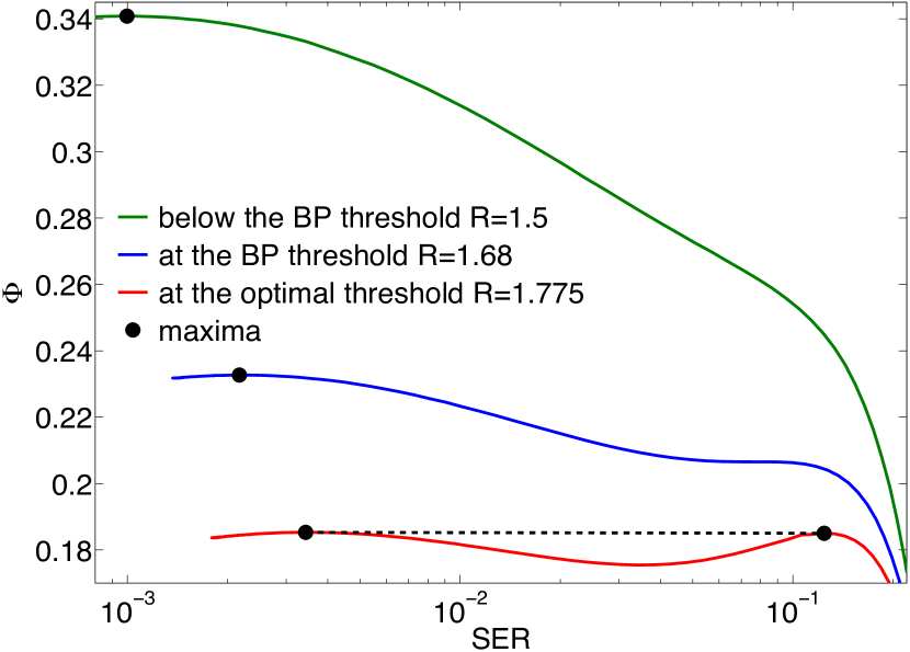
Figure 1: The free-entropy (or potential) $\Phi$ as a function of the section-error rate ${\rm{SER}}$ for $B=2$ and ${\rm{snr}}=30$. The global maximum of the curves allows to identify the typical optimal ${\rm{SER^{*}}}$ of the codes. The curves are obtained by numerical integration of (7). Here for rates larger than $R>1.775$, the optimal ${\rm{SER^{*}}}$ jumps from a low value to a large $O(1)$ one (red curve). This defines the maximum possible rate (to compare here to $C=2.4771$) below which acceptable performance can be obtained. For $R<1.775$, the ${\rm{SER^{*}}}$ is much lower (and decay with $R$). The AMP decoder described in Sec. III allows to perform an ascent of this function. As long as the maximum is unique (i.e. for $R<1.68$, see blue curve), it will be able to achieve the predicted optimal performance in the large size limit.

Let us first access the performances of these codes when $B$ is finite in the large $L\!\to\!\infty$ limit. We proceed as in the LDPC case [7] and define the "potential" function (or free-entropy [9]) at fixed $B$ as $\Phi_{B}\!\vcentcolon=\!\langle\log Z(Y,F)\rangle_{X,F,\xi}$ where $\langle\rangle_{u}$ denotes the average over the random variable $u$ and $Z(Y,F)$ is the normalization of the probability measure of the estimator $\hat{X}$:

$$P_{Y,F}(\hat{X})=\frac{1}{Z(Y,F)}\prod_{l=1}^{L}P_{0}(\hat{\overline{x}}_{l})\prod_{\mu=1}^{M}e^{-\frac{{\rm{snr}}}{2}(y_{\mu}-\sum_{i=1}^{N}F_{\mu i}\hat{x}_{i})^{2}}$$ (2)

where $\hat{\overline{x}}_{l}=[\hat{x}_{1},\hat{x}_{2},...,\hat{x}_{B}]_{l}$ is the $l^{th}$ $B$-d variable of the estimator (i.e one of its $L$ sections as for $\overline{X}$). Our computation is based on the replica method, an heuristic coming from the statistical physics of disordered systems that relies on the identity $\langle\log Z(u)\rangle_{u}=\lim_{n\!\to\!0}(\langle Z(u)^{n}\rangle_{u}-1)/n$ to compute averages of logarithms, and that has been applied very often to coding theory [9], sparse estimation [13, 14, 6, 12] or optimization problems [8] where it has been later shown to rigorously give the correct answer. We shall not give a detailed description of our computation that in fact follows the one given in [12] for compressed sensing almost step by step. The only difference is again that we are dealing here with $B$-d variables $\overline{x}_{l}$ whose components takes binary value $\in\{0,{\rm{val}}_{l}\}$, and only one of the $B$ $x_{i}$’s in $\overline{x}_{l}$ is non zero. Any value ${\rm{val}}_{l}\neq 0$ is a possible choice (such as the exponentially distributed ${\rm{val}}_{l}$ of [1, 10]) but we shall here restrict ourselves to the simplest case where ${\rm{val}}_{l}=1\ \forall\ l\in\{1,...,L\}$. We have observed empirically that this seems to be an efficient distribution for the algorithm we describe in Sec. III.

The estimator we are interested in is the section-error rate (${\rm{SER}}$), the fraction of incorrectly decoded sections:

$${\rm{SER}}\vcentcolon=\frac{1}{L}\sum_{l=1}^{L}\mathbb{I}\left({\rm{argmax}}[P(\hat{\overline{x}}_{l})]\neq\overline{x}_{l}\right)$$ (3)

$${\rm{argmax}}[P(\hat{\overline{x}}_{l})]=[\hat{x}_{1},\hat{x}_{2},...,\hat{x}_{B}]_{l}$$ (4)

$$\hat{x}_{i}\vcentcolon=\mathbb{I}\left(a_{i}>a_{j}\ \forall j\in l:j\neq i\right)$$ (5)

where $a_{i}$ is the posterior average with respect to (2) of the $1$-d variable $x_{i}$, $P(\hat{\overline{x}}_{l})$ is the marginal probability of section $l$ (i.e the joint probability $P(\{\hat{x}_{i}:i\in l\})$) and $\mathbb{I}()$ is the indicator function. Most of our results, however, can be expressed more conveniently as function of a different estimator that we shall denote as the biased MSE $\tilde{E}$:

$$\tilde{E}\vcentcolon=\frac{1}{N}\sum_{i=1}^{N}(a_{i}-x_{i})^{2}$$ (6)

Both quantities behave similarly in our computations. In fact, the replica and DE analysis show that the ${\rm{SER}}$ can be computed directly from the value of $\tilde{E}$ (see Sec. IV, and in particular eq.(18)).

The main interest of the potential is that the actual typical value $\tilde{E}^{*}$ (and thus the typical value ${\rm{SER^{*}}}$) for a given ensemble of codes in the large signal size limit is obtained by maximizing it so that $\tilde{E}^{*}={\rm{argmax}}[\Phi(\tilde{E})]$. After computation and defining a rescaled biased MSE $E\vcentcolon=\tilde{E}B$ one can show that for a given $B$ and up to constants, the potential reads:

$$\Phi_{B}(E)=-\frac{\log_{2}(B)}{2R}\left(\log(1/{\rm{snr}}+E)+\frac{1-E}{1/{\rm{snr}}+E}\right)$$

$$+\int\mathcal{D}\overline{z}\log\left(e^{\frac{1}{2\Sigma(E)^{2}}+\frac{z_{1}}{\Sigma(E)}}+\sum_{i=2}^{B}e^{-\frac{1}{2\Sigma(E)^{2}}+\frac{z_{i}}{\Sigma(E)}}\right)$$ (7)

where $\Sigma(E)\vcentcolon=\sqrt{(1/{\rm{snr}}+E)R/\log_{2}(B)}$ and $\mathcal{D}\overline{z}\vcentcolon=\prod_{i=1}^{B}\mathcal{D}z_{i}$ (with $\mathcal{D}z_{i}$ being a centered Gaussian measure of unit variance). Using the mapping from $\tilde{E}$ to ${\rm{SER}}(\tilde{E})$ given by eq.(18) we can compute numerically $\Phi_{B}({\rm{SER}})$. Exemples are shown in Fig. 1 in the $B\!=\!2$ case for different rates.

Interestingly, the potential behaves very similarly to the one of LDPC codes so that we observed the very same phenomenology. For large enough rates, it develops a "two-maxima shapes" with a high and low error maxima. The low error maxima dominates as long as it is the higher one, i.e statistically dominant. When the two maxima of $\Phi_{B}$ have same height (red curve on Fig. 1) the reconstruction capacities become extremely poor: this mark what we shall refer to as the "optimal threshold", as it represents the point until which the code has good performance under optimal decoding.

It is well known in LDPC codes that the rate for which the second maxima appears (blue curve on Fig. 1) corresponds to the moment where the BP decoder does not correspond anymore to the optimal one. We shall see that this remains the case here and that only in the one-maxima region (green curve on Fig. 1), our AMP decoder will match asymptotically the optimal performance. Fig. 2 represents these two thresholds in the limit $L\!\to\!\infty$ as a function of the section size $B$ for fixed ${\rm{snr}}=15$. We shall come back to the BP performances, but let us first notice here that (i) as $B$ increases, the optimal threshold approaches the Shannon capacity (and in fact the corresponding value of ${\rm{SER}}$ goes to zero, see Fig 4). However, (ii) the rate at which we expect message passing algorithms to converge to the optimal value unfortunately decays as $B$ gets larger. These two observations are in agreament with the $B\!\to\!\infty$ limit, performed by replica analysis: The optimal threshold matches the capacity, as predicted in [1] and the rate at the BP threshold is asymptotically given by:

$$R_{BP}\underset{L\to\infty}{=}[(1/\rm{snr}+1)2\log 2]^{-1}$$ (8)

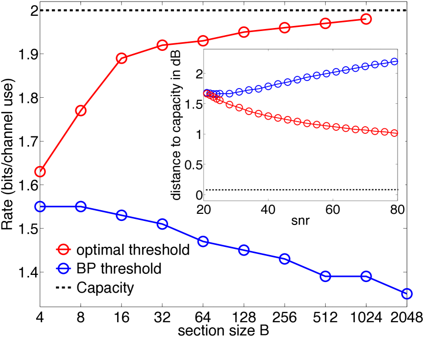
Figure 2: Main Fig: Phase diagram for ${\rm{snr}}=15$ changing $B$. The two transition lines (blue and red) are respectively the BP threshold and the optimal one (see Fig. 1). At the optimal transition the ${\rm{SER^{*}}}$ drops from $O(1)$ values to much lower ones. Below the BP threshold, the optimal ${\rm{SER^{*}}}$ is achievable using the AMP decoder described in Sec. III. Notice that while the optimal threshold tends to the capacity $C$ as $B$ increases, the BP threshold unfortunately decays when $B$ increases. Inset: Phase diagram with the same transitions plotted in distance in dB from capacity at fixed $B\!=\!2$ and changing the ${\rm{snr}}$. Below ${\rm{snr}}\approx 20$, there are no more transition and the ${\rm{SER}}$ decreases continuously with the rate. Curves are obtained by Monte Carlo integration with sample size of $10^{6}$ of eq.(7) and eq.(18) for $B>2$ and direct numerical integration for $B\!=\!2$.

III Approximate Message Passing algorithm

We shall now consider a BP type iterative algorithm to estimate the joint probability $P(\hat{\overline{x}}_{l})$ of one section, still in the case where ${\rm{val}}_{l}=1\ \forall\ l$. Following the derivation of the AMP in [12], it follows from the parametrization:

$$P(\hat{\overline{x}}_{l}) =\frac{P_{0}(\hat{\overline{x}}_{l})}{z}\prod_{\{i\in l\}}^{B}m(\hat{x}_{i})$$ (9)

$$z =\sum_{\{i\in l\}}^{B}e^{-\frac{(1-R_{i})^{2}}{2\Sigma_{i}^{2}}}\prod_{j\neq i}^{B-1}e^{-\frac{R_{j}^{2}}{2\Sigma_{j}^{2}}}$$ (10)

$$P_{0}(\hat{\overline{x}}_{l}) =\frac{1}{B}\sum_{\{i\in l\}}^{B}\delta(\hat{x}_{i}-1)\prod_{j\neq i}^{B-1}\delta(\hat{x}_{j})$$ (11)

where $P_{0}()$ is the prior that matches the signal distribution, eq.(2). This matching condition is called Nishimori condition in statistical physics [15, 12]. The set $\{m(\hat{x}_{i})\sim\mathcal{N}_{R_{i},\Sigma^{2}_{i}}\}$ are Gaussian distributed, with moments iteratively computed by the AMP. Marginalizing over $\{\hat{x}_{j}\in\hat{\overline{x}}_{l}\neq\hat{x}_{i}\}$ we get after simplification the posterior average $a_{i}^{t}$ and variance $v_{i}^{t}$ of $\hat{x}_{i}$ at step t of the algorithm:

$$a_{i}^{t} \vcentcolon=f_{a_{i}}(\{\Sigma_{j}^{t},R_{j}^{t}\}_{j\in l})=\frac{e^{-\frac{1-2R_{i}^{t}}{2(\Sigma_{i}^{t})^{2}}}}{\sum_{\{j\in l\}}^{B}e^{{-\frac{1-2R_{j}^{t}}{2(\Sigma_{j}^{t})^{2}}}}}$$ (12)

$$v_{i}^{t} \vcentcolon=f_{c_{i}}(\{\Sigma_{j}^{t},R_{j}^{t}\}_{j\in l})=a_{i}^{t}(1-a_{i}^{t})$$ (13)

AMP allows to obtain the estimate at time $t$ given the parametrization (9) as follows (see again [12]):

$$\boxed{\begin{aligned} V^{t+1}_{\mu}&=\sum_{i}F_{\mu i}^{2}v_{i}^{t}\\ \omega^{t+1}_{\mu}&=\sum_{i}F_{\mu i}a^{t}_{i}-(y_{\mu}-\omega^{t}_{\mu})\frac{V^{t+1}_{\mu}}{1/{\rm{snr}}+V^{t}_{\mu}}\ \ \\ (\Sigma^{t+1}_{i})^{2}&=\left[\sum_{\mu}\frac{F^{2}_{\mu i}}{1/{\rm{snr}}+V^{t+1}_{\mu}}\right]^{-1}\\ R^{t+1}_{i}&=a^{t}_{i}+(\Sigma^{t+1}_{i})^{2}\sum_{\mu}F_{\mu i}\frac{(y_{\mu}-\omega^{t+1}_{\mu})}{1/{\rm{snr}}+V^{t+1}_{\mu}}\ \ \\ a^{t+1}_{i}&=f_{a_{i}}\left(\{\Sigma_{j}^{t+1},R_{j}^{t+1}\}_{j\in l}\right)\\ v^{t+1}_{i}&=f_{c_{i}}\left(\{\Sigma_{j}^{t+1},R_{j}^{t+1}\}_{j\in l}\right)\end{aligned}}$$

Here only the functions $f_{a_{i}}()$ and $f_{c_{i}}()$ depend in an explicit way on the signal model $P_{0}()$. A suitable initialization for the quantities is ($a_{i}^{t=0}\!=\!0$, $v_{i}^{t=0}\!=\!1/(B{\rm{snr}})$, $\omega_{\mu}^{t=0}\!=\!y_{\mu}$). Once the convergence of the iterative equations is reached, one get the posterior average of the $i^{th}$ signal component given by $a^{t}_{i}$ and the ${\rm{SER}}^{t}$ as well using ${\rm{argmax}}[P(\hat{\overline{x}}_{l}^{t})]$, eq.(4).

IV Asymptotic analysis of AMP

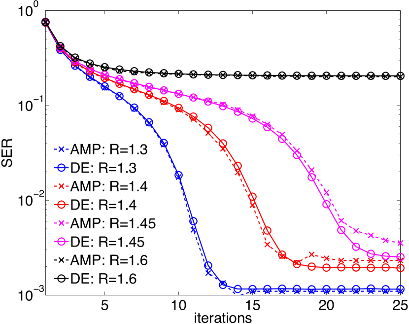
Figure 3: The density evolution predictions of the ${\rm{SER}}^{t}$ for $t\geq 1$ (${\rm{SER}}^{t=0}=1$) compared to the actual one of the algorithm for ${\rm{snr}}=15$ and different rates (to be compared to the BP threshold at $R_{BP}=1.55$) and a section size $B\!=\!4$. DE is computed by a Monte Carlo technique with a sample size of $10^{7}$ and the signal size for AMP is $N=2^{15}$. The figure shows how close is the prediction from the true behavior for finite sizes.

The dynamics of the ${\rm{SER}}^{t}$ under the AMP recursions can be described in the large signal size ($N\!\to\!\infty$, $L\!\to\!\infty$, $B\!=\!N/L$ fixed) using the DE technic [4]. It consists in the statistical analysis of the quantities $(a_{i}^{t},v_{i}^{t})$, which is based on the fact that the product in (9) becomes Gaussian distributed (by central-limit theorem) as $L\to\infty$.

As for the replica analysis, our derivation follows [12] with the only difference that we are dealing with $B$-d variables. Defining the effective variance $\Sigma^{t}$ and the rescaled biased MSE as in (6) which now depends on the iteration step:

$$\Sigma^{t}\vcentcolon=\sqrt{(1/{\rm{snr}}+E^{t})R/\log_{2}(B)},\ E^{t}\vcentcolon=\frac{1}{L}\sum_{i=1}^{N}(a_{i}^{t}-x_{i})^{2}$$ (14)

then the rescaled biased MSE follows the following iteration in the $L\!\to\!\infty$ limit:

$$E^{t}\!\!=\!\!\int\!\!\mathcal{D}\overline{z}\left([f_{a_{1}}^{(1)}(\Sigma^{t-1},\overline{z})-1]^{2}+(B-1)[f_{a_{1,2}}^{(0)}(\Sigma^{t-1},\overline{z})]^{2}\right)$$ (15)

where:

$$f_{a_{i}}^{(1)}(\Sigma,\overline{z}) \vcentcolon=\left[1+e^{-\frac{1}{\Sigma^{2}}}\!\!\!\!\!\!\!\!\sum_{\{1\leq j\leq B:j\neq i\}}\!\!\!\!\!\!\!\!e^{\frac{z_{j}-z_{i}}{\Sigma}}\right]^{-1}$$ (16)

$$f_{a_{i,j}}^{(0)}(\Sigma,\overline{z}) \vcentcolon=\left[1+e^{\frac{1}{\Sigma^{2}}+\frac{z_{j}-z_{i}}{\Sigma}}+\!\!\!\!\!\!\!\!\sum_{\{1\leq k\leq B:k\neq i,j\}}\!\!\!\!\!\!\!\!\!\!e^{\frac{z_{k}-z_{i}}{\Sigma}}\right]^{-1}$$ (17)

In this approach, there is a one to one correspondance from the value of the biased MSE to the ${\rm{SER}}$ thanks to the mapping:

$${\rm{SER}}^{t}\!\!=\!\!\int\!\mathcal{D}\overline{z}\ \mathbb{I}\left(\exists\ j\in\{2,...,B\}:f_{a_{j,1}}^{(0)}(\Sigma^{t},\overline{z})>f_{a_{1}}^{(1)}(\Sigma^{t},\overline{z})\right)$$ (18)

The fixed-point of this set of equations for a given $B$, starting from $E^{t=0}\!=\!1$, allows to compute the asymptotic ${\rm{SER}}$ reached after convergence. Fig. 3 compares the DE prediction of the ${\rm{SER}}^{t}$ versus the algorithm dynamics in the $B\!=\!4$ case for different rates. We see how close is the DE asymptotic theory from the true behavior even for small signals.

Finally, let us now comment on the classical duality between DE results and the replica potential: DE equations are nothing but the fixed point iterations of the replica potential [9]. As discussed in the Sec. II we thus now can identify the BP threshold studied in Sec. II as the moment where the DE iterations remain confined in high ${\rm{SER}}$ values.

Figure 4: Density Evolution prediction of the optimal ${\rm{SER^{*}}}$ at fixed rate $R=1.3$. The red curve is function of $B$ at fixed ${\rm{snr}}=15$, the blue one at fixed $B\!=\!2$ as a function of the ${\rm{snr}}$. The plots are in double logarithmic scale. The line is a power law fit to guide the eyes ( ${\rm{SER^{*}}}(B)\propto B^{-3.76}$ and ${\rm{SER^{*}}}({\rm{snr}})\propto{\rm{snr}}^{-7.25}$).

What have we learned from this analysis? The main point is stressed in Fig. 2: the BP threshold goes to larger distance from capacity as $B$ increases. This is unfortunate since, as shown in Fig. 4, the optimal ${\rm{SER^{*}}}$ decays drastically when $B$ is increased. Nevertheless, AMP alone is not able to reach optimal performance for high rates.

V Numerical experiments

The previous sections were asymptotic studies of the AMP performances. In this section we study numerically the influence of finite size effects over the performance of superposition codes combined with the AMP decoder. Fig. 5 summarizes our findings. We have limited ourselves to small sizes and performed some numerical protocols to test the iterative AMP decoding. We checked that not only the Bayesian decoder does follow the density evolution, but it works very well for limited size as well, at least far enough from the BP threshold. In fact, when the rate is below the threshold, the decoding is usually perfect and is found to reach with high probability ${\rm{SER}}\!=\!0$. This is due to the fact that in order to observe an ${\rm{SER}}\in O(\epsilon)$, there must be at least $L\approx 1/\epsilon$ sections which is not the case for small signals, when the asymptotic ${\rm{SER}}$ is very small. Even for reasonably large sizes allowing to get close to the asymptotic performances (such as $L\!=\!2000$, green curve on Fig. 5), AMP just take seconds to decode on a Matlab code.

To confirm that the relevant parameter with respect to the finite size effects is $L$ and not $N$, we made the following experiment (protocol 1 in Fig. 5) fixing $N$ and varying $B$ (thus $L$ decreases as $B$ increases) and observed that the performances worsen rapidly as $B$ increases.

Finally we compared the efficiency of AMP to the iterative successive decoder introduced by Baron and Joseph [1]. This decoder has been shown to be capacity achieving in the large $B$ limit for a slightly different version of the superposition codes, when an exponential distribution of the signal entries (see Sec. II) is used instead of the $\{0,1\}$ distribution we have been studying. However, the finite $B$ corrections to the performance appear to be quite severe. We have compared the performance of our approach (with the $\{0,1\}$ distribution) with the result obtained in [1] (see again Fig. 5) and found that at the values of $B$ that one can consider in a computer, AMP appears to be superior in performance (though it will eventually be outperformed it in the limit of very large values of $B$). This remains the case even when compared to the most recent developements [16]. It would be interesting to actually find what is the best possible signal distribution to further optimize the performances of AMP reconstruction.

Figure 5: Numerical experiment at finite limited sizes $L$ for ${\rm{snr}}=15$. The blue line is the BP threshold rate predicted by the density evolution technic (to be compared to $C=2$, see Fig. 2) and marks the limit of efficiency of AMP for large signals. Here we limit ourselves to small signals in order to compare with other results in the literature. All the curves with crosses are results of the following protocol (protocol 1): decode $10^{4}$ random instances and identify the transition line between a phase where the probability $p_{\epsilon}$ to have a ${\rm{SER}}>10^{-1}$ is $p_{\epsilon}<10^{-3}$ (below the line) from a phase where $p_{\epsilon}\geq 10^{-3}$ (more than 9 instances have failed over the $10^{4}$ ones). The squared line is the result of the second protocol (protocol 2): at the first try, we require ${\rm{SER}}<10^{-1}$ for $10$ random instances in a row below the line, not above. Note that in our experiments ${\rm{SER}}<10^{-1}$ essentially means ${\rm{SER}}=0$ at these sizes. We compare our results with the iterative successive decoder of [1, 10] in protocol 1 where the number of sections $L=100$ (note that these data, taken from [1, 10], have been generated with a code with an exponential signal distribution rather than the $\{0,1\}$ we used here in order to increase the quality of the reconstruction). Compared with the red curve (AMP with the same value of $L$) the better quality of AMP reconstruction is clear. For both the experimental and asymptotic performances of AMP, the maximum number of iterations of the algorithm is arbitrarily fixed to $50$.

VI Perspectives

We have provided here a replica analysis of superposition codes and a Bayesian approximate message passing decoder based on a belief-propagation like approach that we have analyzed using the density evolution technic. We have found a behavior very similar to those found in LDPC codes. In particular, our AMP decoder seems to have good performances, but is limited to region far from optimal decoding. We have released a Matlab implementation of our decoder at https://github.com/jeanbarbier/BPCS_common.

There are a number of possible continuations of the present work, in the spirit of recent developments in compressed sensing. Superposition codes which lies on the fuzzy separation between coding and compressed sensing theories are in fact a natural venue for these ideas. The most natural one is to use the spatial coupling approach [17, 18, 19] in order to design codes with exact optimal performances but for which AMP will be able to achieve them for all rates. This strategy is known to work in compressed sensing [12, 6, 20] so that its application in the present context should be straightforward. Another interesting direction would be to replace the random matrices used in this work by structured ones allowing a fast multiplication, as it has been done, again, in compressed sensing [21, 22], in order to have a decoder as fast as those used in sparse codes. We plan to study these points in a future work.

References

- [1] A. R. Barron and A. Joseph, “Sparse superposition codes: Fast and reliable at rates approaching capacity with gaussian noise,” Manuscript. Available at “http://www. stat. yale. edu/ arb4, 2010.
- [2] A. Joseph and A. R. Barron, “Least squares superposition codes of moderate dictionary size are reliable at rates up to capacity,” Information Theory, IEEE Transactions on, vol. 58, no. 5, pp. 2541–2557, 2012.
- [3] D. L. Donoho, A. Maleki, and A. Montanari, “Message-passing algorithms for compressed sensing,” Proc. Natl. Acad. Sci., vol. 106, no. 45, pp. 18 914–18 919, 2009.
- [4] M. Bayati and A. Montanari, “The dynamics of message passing on dense graphs, with applications to compressed sensing,” IEEE Transactions on Information Theory, vol. 57, no. 2, pp. 764 –785, 2011.
- [5] S. Rangan, “Generalized approximate message passing for estimation with random linear mixing,” in IEEE International Symposium on Information Theory Proceedings (ISIT), 2011, pp. 2168 –2172.
- [6] F. Krzakala, M. Mézard, F. Sausset, Y. Sun, and L. Zdeborová, “Statistical physics-based reconstruction in compressed sensing,” Phys. Rev. X, vol. 2, p. 021005, 2012.
- [7] T. Richardson and R. Urbanke, Modern Coding Theory. Cambridge University Press, 2008.
- [8] M. Mézard, G. Parisi, and M. A. Virasoro, Spin-Glass Theory and Beyond. Singapore: World Scientific, 1987, vol. 9.
- [9] M. Mézard and A. Montanari, Information, Physics, and Computation. Oxford: Oxford Press, 2009.
- [10] A. R. Barron and A. Joseph, “Analysis of fast sparse superposition codes,” in Information Theory Proceedings (ISIT), 2011 IEEE International Symposium on. IEEE, 2011, pp. 1772–1776.
- [11] A. Montanari, “Graphical models concepts in compressed sensing,” Compressed Sensing: Theory and Applications, pp. 394–438, 2012.
- [12] F. Krzakala, M. Mézard, F. Sausset, Y. Sun, and L. Zdeborová, “Probabilistic reconstruction in compressed sensing: Algorithms, phase diagrams, and threshold achieving matrices,” J. Stat. Mech., 2012.
- [13] T. Tanaka, “A statistical-mechanics approach to large-system analysis of cdma multiuser detectors,” IEEE Trans. Infor. Theory, vol. 48, pp. 2888–2910, 2002.
- [14] Y. Kabashima, T. Wadayama, and T. Tanaka, “A typical reconstruction limit of compressed sensing based on lp-norm minimization,” J. Stat. Mech., p. L09003, 2009.
- [15] H. Nishimori, Statistical Physics of Spin Glasses and Information Processing. Oxford: Oxford University Press, 2001.
- [16] A. R. Barron and S. Cho, “High-rate sparse superposition codes with iteratively optimal estimates,” in Information Theory Proceedings (ISIT), 2012 IEEE International Symposium on. IEEE, 2012, pp. 120–124.
- [17] S. Kudekar, T. Richardson, and R. Urbanke, “Spatially coupled ensembles universally achieve capacity under belief propagation,” 2012, arXiv:1201.2999v1 [cs.IT].
- [18] ——, “Threshold saturation via spatial coupling: Why convolutional ldpc ensembles perform so well over the bec,” in Information Theory Proceedings (ISIT),, 2010, pp. 684–688.
- [19] A. Yedla, Y.-Y. Jian, P. S. Nguyen, and H. D. Pfister, “A simple proof of threshold saturation for coupled scalar recursions,” 2012, arXiv:1204.5703v1 [cs.IT].
- [20] D. L. Donoho, A. Javanmard, and A. Montanari, “Information-theoretically optimal compressed sensing via spatial coupling and approximate message passing,” in Proc. of the IEEE Int. Symposium on Information Theory (ISIT), 2012.
- [21] A. Javanmard and A. Montanari, “Subsampling at information theoretically optimal rates,” in Information Theory Proceedings (ISIT), 2012 IEEE International Symposium on, July 2012, pp. 2431–2435.
- [22] J. Barbier, F. Krzakala, and C. Schülke, “Compressed sensing and approximate message passing with spatially-coupled fourier and hadamard matrices,” arXiv preprint arXiv:1312.1740, 2013.