Optimal Power Allocation for Three-phase Bidirectional DF Relaying with Fixed Rates

Abstract

Wireless systems that carry delay-sensitive information (such as speech and/or video signals) typically transmit with fixed data rates, but may occasionally suffer from transmission outages caused by the random nature of the fading channels. If the transmitter has instantaneous channel state information (CSI) available, it can compensate for a significant portion of these outages by utilizing power allocation. In this paper, we consider optimal power allocation for a conventional dual-hop bidirectional decode-and-forward (DF) relaying system with a three-phase transmission protocol. The proposed strategy minimizes the average power consumed by the end nodes and the relay, subject to some maximum allowable system outage probability (OP), or equivalently, minimizes the system OP while meeting average power constraints at the end nodes and the relay. We show that in the proposed power allocation scheme, the end nodes and the relay adjust their output powers to the minimum level required to avoid outages, but will sometimes be silent, in order to conserve power and prolong their lifetimes. For the proposed scheme, the end nodes use the instantaneous CSI of their respective source-relay links and the relay uses the instantaneous CSI of both links.

I Introduction

Compared to unidirectional relaying, bidirectional (two-way) relaying is a more suitable alternative for applications where the end nodes intend to exchange information (e.g., in interacive applications) [1]. Bidirectional relaying is also spectrally more efficient than unidirectional relaying, because it exploits the broadcast nature of the wireless medium [2]. The relay combines two unidirectional unicast transmissions into a single broadcast transmission using the network coding concept [3]. The time-division broadcast (TDBC) protocol is the most important three-phase bidirectional decode-and-forwad (DF) relaying scheme. It increases spectral efficiency by 33% compared to unidirectional relaying [4].

Papers [5] and [6] study the capacity outage probability (OP) of the TDBC protocol. The OP well describes the behaviour of a system that operates at fixed information rates over quasi-static (i.e., slowly fading) channels, where the rate is selected such that each codeword is transmitted over one channel realization. Fixed-rate communication is suitable for delay-sensitive applications, such as, bidirectional interactive speech and/or video communication. However, [5] and [6] assume that the end nodes and the relay transmit at fixed output powers, although they have to have instantaneous channel state information (CSI) available as this is required for decoding. Apart from decoding, this CSI can also be used for power adaptation at the relay and the end nodes such that outage minimization is achieved under some (long-term) average power constraint. Unlike the more restrictive short-term power constraint that limits the codeword power for each channel realization, the average power constraints limit the average power of all codewords over all channel realizations [10]. For point-to-point channels, such power adaptation is known as truncated channel inversion and has been introduced in [9]. For unidirectional relaying, optimal power allocation for source and relay has been studied for both conventional amplify-and-forward [7] and decode-and-forward (DF) [8] relaying systems under various average power constraints. Optimal power allocation has been shown to introduce significant performance improvement relative to constant power transmissions [7]-[10]. However, literature does not offer similar results for bidirectional relaying.

In this work, we derive power control strategyies for the end-nodes and the relay in three-phase bidirectional DF relaying. For predefined constant rates in both directions, the proposed power allocation achieves minimization of the system OP assuming individual average power constraints at the end nodes and the relay. For the power allocation, the end nodes use the instantaneous CSI of their respective source-relay links and the relay uses the instantaneous CSI of both links. Intuitively, it is not necessary for the end nodes and the relay to transmit at their maximum available power in each transmission cycle, but transmit with the minimum power required to avoid outages, or sometimes even be silent when an outage is unavoidable, thus conserving their power. In other words, we allow outages to occur in cases of deep fades, but for the rest of the time we ensure successful transmissions at the predefined constant transmission rate.

II System and channel model

The considered bidirectional relaying system consists of two end-nodes ($S_{1}$ and $S_{2}$) and a half-duplex DF relay $R$. The bidirectional communication consists of two parallel unidirectional communication sessions, $S_{1}\rightarrow S_{2}$ and $S_{2}\rightarrow S_{1}$. Each communication session is realized at a fixed information rate, $R_{01}$ and $R_{02}$, respectively. We assume the direct $S_{1}-S_{2}$ link is not available, thus, the bidirectional communication is realized only via the relayed link. The OP for this system is defined as the probability that at least one (or both) of the communications sessions is in outage.

The squared amplitudes of the $S_{1}-R$ and $S_{2}-R$ channels are denoted by $x$ and $y$, and have arbitrary average values $\Omega_{X}$ and $\Omega_{Y}$, respectively. We assume that the $R-S_{1}$ channel is reciprocal to the $S_{1}-R$ channel, and the $R-S_{2}$ channel is reciprocal to the $S_{2}-R$ channel. We adopt the Rayleigh block fading model, which means that the values of $x$ and $y$ are constant within each transmission cycle, but change from one transmission cycle to the next. Thus, in each transmission cycle, the pair $\left(x,y\right)$ denotes the channel state, where both $x$ and $y$ follow the Rayleigh probability distribution function (PDF).

Each transmission cycle is divided into three phases: In phase 1, $S_{1}$transmits its codeword $s_{1}(t)$ at information rate $R_{01}$ with an output power $P_{S1}\left(x\right)$, and the DF relay receives. In phase 2, $S_{2}$ transmits its codeword $s_{2}(t)$ at information rate $R_{02}$ with an output power $P_{S2}\left(y\right)$, and the DF relay receives. The relay attempts to decode both codewords $s_{1}(t)$ and $s_{2}(t)$. If it successfully decodes both of them, the relay generates a single composite codeword that carries the information of both $s_{1}(t)$ and $s_{2}(t)$ [2]. Then, in phase 3, the relay broadcasts the composite codeword towards the end nodes with an output power $P_{R}\left(x,y\right)$.

Note that the output powers from the end nodes and the relay have been written as functions of the channel state. In each transmission cycle, node $S_{1}$ is assumed to know only the value of $x$, whereas node $S_{2}$ is assumed to know only the value of $y$. Based on this CSI knowledge, each end node can ”subtract” its own codeword from the received codeword, and then attempt to decode the noisy version of the codeword that originates from the other node. The DF relay can decode both codewords since it is assumed to know both $x$ and $y$. The received signals at the end nodes and the relay are corrupted by additive white Gaussian noise (AWGN) with zero mean and unit variance.

We present optimal power allocation (OPA) strategies at the end nodes and the relay that minimize the system OP, subject to the individual average power constraints $\overline{P}_{S1}$, $\overline{P}_{S2}$, and $P_{avg}$ at $S_{1}$, $S_{2}$, and the relay. In phase 1, $S_{1}$ uses power control based on its knowledge of $x$ so as to achieve truncated channel inversion of the $S_{1}-R$ channel at rate $R_{01}$ [9]. Similarly, in phase 2, $S_{2}$ uses power control based on its knowledge of $y$ so as to achieve truncated channel inversion of the $S_{2}-R$ channel at rate $R_{02}$. In phase 3, if both codewords $s_{1}(t)$ and $s_{2}(t)$ are successfully decoded by the relay, the adopted power control mechanism minimizes the OP over the broadcast channel (Section IV).

III Power control at the end nodes

The $S_{1}-R$ channel can support $S_{1}$’s transmission rate, $R_{01}$, if the instantaneous capacity of the channel between $S_{1}$ and the relay exceeds this rate,

$$\frac{1}{3}\log(1+P_{S1}x)\geq R_{01}\text{,}$$ (1)

where the the pre-log factor $1/3$ is due to the three-phase transmission cycle. For an available average power of end node $S_{1}$ of $\overline{P}_{S1}$, the OPA strategy at $S_{1}$ is given by [8]

$$P_{S1}(x)=\left\{\begin{array}[]{c}\frac{\delta_{1}}{x},\text{ \ }x\geq x_{0}\\ 0,\text{ \ }x<x_{0}\end{array}\right.\text{,}$$ (2)

where $\delta_{1}=2^{3R_{01}}-1$. In (2), the cutoff threshold $x_{0}$ is determined from

$$\overline{P}_{S1}=\int_{x_{0}}^{\infty}\frac{\delta_{1}}{x}f_{X}\left(x\right)dx=\frac{\delta_{1}}{\Omega_{X}}E_{1}\left(\frac{x_{0}}{\Omega_{X}}\right)\text{.}$$ (3)

The right hand side of (3) is valid for Rayleigh fading, where $E_{1}\left(\cdot\right)$ is the exponential integral function [11]. Analogously, the $S_{2}-R$ channel can support $S_{2}$’s transmission rate, $R_{02}$, with its average output power $\overline{P}_{S2}$, if the instantaneous capacity of the channel between $S_{2}$ and the relay exceeds this rate,

$$\frac{1}{3}\log(1+P_{S2}y)\geq R_{02}$$ (4)

which leads to the OPA strategy at $S_{2}$,

$$P_{S2}(y)=\left\{\begin{array}[]{c}\frac{\delta_{2}}{y},\text{ \ }y\geq y_{0}\\ 0,\text{ \ }y<y_{0}\end{array}\right.\text{,}$$ (5)

where $\delta_{2}=2^{3R_{02}}-1$. The corresponding cutoff threshold $y_{0}$ is determined from

$$\overline{P}_{S2}=\int_{y_{0}}^{\infty}\frac{\delta_{2}}{y}f_{Y}\left(y\right)dy=\frac{\delta_{2}}{\Omega_{Y}}E_{1}\left(\frac{y_{0}}{\Omega_{Y}}\right)\text{.}$$ (6)

IV Power control at the relay

Considering (2) and (5), the relay successfully decodes both codewords $s_{1}(t)$ and $s_{2}(t)$ only if $\left(x,y\right)\in D_{R}$, where $D_{R}$ is the relay’s non-outage region defined as

$$D_{R}\text{: \ \ \ \ }x\geq x_{0}\text{ and }y\geq y_{0}.$$ (7)

In this case, the relay generates the composite signal, and, in phase 3 broadcasts the composite codeword towards the end nodes with an output power $P_{R}\left(x,y\right)$.

Theorem 1

The solution of the optimization problem

$$\text{$\underset{P_{R}\left(x,y\right)}{\text{minimize}}$ }P_{R}\left(x,y\right)$$

$$\text{subject to \ \ }\frac{1}{3}\log_{2}\left(1+P_{R}\left(x,y\right)\text{ }y\right) \geq R_{01}$$

$$\frac{1}{3}\log{}_{2}\left(1+P_{R}\left(x,y\right)\text{ }x\right) \geq R_{02}$$

$$x\geq x_{0}\text{ and }y\geq y_{0}$$ (8)

is given by

$$P_{R,st}\left(x,y\right)=\left\{\begin{array}[]{c}\max\left\{\frac{\delta_{1}}{y},\frac{\delta_{2}}{x}\right\},\text{ \ }x\geq x_{0}\text{ and }y\geq y_{0}\\ 0,\text{ otherwise}\end{array}\right..$$ (9)

Proof:

Optimization problem (8) is a standard linear programming (LP) problem, whose solution is feasible because the intersection of the constraints is a non-empty set, and it lies at the boundary of the intersection, given by (9). This concludes the proof. ∎

If the relay successfully decodes both codewords, i.e., $\left(x,y\right)\in D_{R}$, the power adaptation (9) guarantees zero outages in the broadcase phase with minimum output power from the relay, because both end nodes can successfully decode their intended codewords in the broadcast phase. If $\left(x,y\right)\notin D_{R}$, the relay should be silent as it cannot decode at least one of the two codewords. Assuming power control accoding to (9), the relay’s non-outage region $D_{R}$ is divided into two non-overlaping regions, $D_{R}=D_{R}^{\prime}\cup D_{R}^{\prime\prime}$, such that

$$D_{R}^{\prime}:\text{ \ \ }x\geq x_{0}\text{ and }y_{0}\leq y\leq\frac{\delta_{1}}{\delta_{2}}x$$ (10)

$$D_{R}^{\prime\prime}:\text{ \ \ }y\geq y_{0}\text{ and }x_{0}\leq x\leq\frac{\delta_{2}}{\delta_{1}}y$$ (11)

If $\left(x,y\right)\in D_{R}^{\prime}$, the relay transmits with power $\delta_{1}/y$, whereas if $\left(x,y\right)\in D_{R}^{\prime\prime}$, the relay transmits with power $\delta_{2}/x$. Figs. 1 and 2 graphically illustrate the non-outage regions $D_{R}^{\prime}$ given by (10) and $D_{R}^{\prime\prime}$ given by (11), where Fig. 1 applies to the case $\delta_{2}y_{0}\leq\delta_{1}x_{0}$ whereas Fig. 2 applies to the case $\delta_{2}y_{0}>\delta_{1}x_{0}$. Thus, the power adaptation (9) can be further decomposed as

$$P_{R,st}\left(x,y\right)=\left\{\begin{array}[]{c}\frac{\delta_{1}}{y},\text{ \ \ }x\geq x_{0}\text{ and }y_{0}\leq y\leq\frac{\delta_{1}}{\delta_{2}}x\\ \frac{\delta_{2}}{x},\text{ \ \ }y\geq y_{0}\text{ and }x_{0}\leq x\leq\frac{\delta_{2}}{\delta_{1}}y\\ 0,\text{ \ \ otherwise}\end{array}\right.\text{ \ .}$$ (12)

Figure 1: Non-outage region for $\delta_{2}y_{0}\leq\delta_{1}x_{0}$

IV-A Outage Minimization

However, even if $\left(x,y\right)\in D_{R}$, it may still be impossible to maintain zero outage probability in the broadcast phase, because the relay is also constrained by its own long-term power budget $P_{avg}$. The system OP is determined as

$$P_{out}=\underset{\left(x,y\right)\in D_{R}}{\int\int}dxdy\text{ }f_{X}\left(x\right)f_{Y}\left(y\right)\qquad\qquad\qquad\qquad\qquad\quad$$

$$\times\Pr\left\{\left.\begin{array}[]{c}\frac{1}{3}\log_{2}\left(1+P_{R}\left(x,y\right)\text{ }y\leq R_{01}\right)\text{ \ }\\ \text{OR \thinspace}\frac{1}{3}\log_{2}\left(1+P_{R}\left(x,y\right)\text{ }x\leq R_{02}\right)\end{array}\right|\left(x,y\right)\in D_{R}\right\}\text{.}$$ (15)

(16)

According to (15), $P_{out}$ can be minimized if both of the following requirements are satisfied: (i) the area of $D_{R}$ is maximized, and (ii) the conditional outage probability in the integrand of (15) is minimized. For the CSI available at the end nodes ($S_{1}$ knows only $x$ and $S_{2}$ knows only $y$), (3) and (6) guarantee that the area of $D_{R}$ is maximized. For requirement (ii), we have the following theorem.

Theorem 2

The solution of optimization problem

$$\text{$\underset{P_{R}\left(x,y\right)}{\text{minimize}}$ }\Pr\left\{\begin{array}[]{c}\text{ \ \ \ \ \ \ }\frac{1}{3}\log_{2}\left(1+P_{R}\left(x,y\right)\text{ }y\right)\leq R_{01}\text{ }\\ \text{OR \ }\frac{1}{3}\log_{2}\left(1+P_{R}\left(x,y\right)\text{ }x\right)\leq R_{02}\end{array}\right\}$$

$$\text{subject to \ \ \ }E_{XY}\left[P_{R}\left(x,y\right)\right]\leq P_{avg}\text{ \ and \ }\left(x,y\right)\in D_{R}\text{,}$$ (17)

where $E_{XY}\left[\cdot\right]$ denotes expectation with respect to $X$ and $Y$, is given by

$$P_{R}^{\ast}\left(x,y\right)=\left\{\begin{array}[]{c}P_{R,st}\left(x,y\right),\text{ \ \ if }P_{R,st}\left(x,y\right)\leq\rho\\ 0,\text{ \ \ \ \ \ \ \ \ \ \ \ \ \ \ \ if }P_{R,st}\left(x,y\right)>\rho\end{array}\right.\text{ ,}$$ (18)

where $P_{R,st}\left(x,y\right)$ is given by (12) and the cutoff threshold $\rho$ is determined from

$$P_{avg}=E_{XY}\left[P_{R,st}\left(x,y\right)\text{ }|P_{R,st}\left(x,y\right)\leq\rho\right]\text{ .}$$ (19)

Proof:

The proof is analogous to [8, Appendix B] and [10, Appendix D], where $P_{R,st}\left(x,y\right)$ is the minimum short-term power of the relay that maintains zero outages in the broadcast phase. ∎

Figure 2: Non-outage region $\delta_{2}y_{0}>\delta_{1}x_{0}$

Combining (18) and (12), the OPA strategy at the relay is finally obtained as

$$P_{R}^{\ast}\left(x,y\right)=\left\{\begin{array}[]{c}\frac{\delta_{1}}{y},\text{ \ }x\geq x_{0}\text{ and }\max\left\{\frac{\delta_{1}}{\rho},y_{0}\right\}\leq y\leq\frac{\delta_{1}}{\delta_{2}}x\\ \frac{\delta_{2}}{x},\text{ \ }y\geq y_{0}\text{ and }\max\left\{\frac{\delta_{2}}{\rho},x_{0}\right\}\leq x\leq\frac{\delta_{2}}{\delta_{1}}y\\ 0,\text{ otherwise}\end{array}\right.\text{ .}$$ (20)

Considering the assumptions for the CSI availability at the end nodes and the relay, the power allocation rules $P_{S1}\left(x\right)$, $P_{S2}\left(y\right)$, and $P_{R}\left(x,y\right)$, given by (3), (5), and (20), respectively, are optimal as they minimize the OP of the three-phase bidirectional DF relaying system for individual power constraints at the end nodes and the relay.

IV-B Average Output Power and Cutoff Threshold $\rho$

The analytical expression for the average relay output power is obtained by statistical averaging of (20) with respect to $x$ and $y$. Let us first introduce two auxiliary variables $\lambda_{1}$ and $\lambda_{2}$, defined as

$$\lambda_{1} = \max\left\{x_{0},\delta_{2}/\rho\right\}\text{, }$$

$$\lambda_{2} = \max\left\{y_{0},\delta_{1}/\rho\right\}\text{.}$$ (21)

a) If $\delta_{2}y_{0}\leq\delta_{1}x_{0}$ (Fig. 1), the average relay output power, $\overline{P}_{R1}$, is expressed as

$$\overline{P}_{R1}\left(\rho\right) = \int\limits_{x_{0}}^{\infty}f_{X}\left(x\right)\int\limits_{\lambda_{2}}^{\frac{\delta_{1}x}{\delta_{2}}}\frac{\delta_{1}}{y}f_{Y}\left(y\right)dydx$$ (22)

$$+\int\limits_{\frac{\delta_{1}\lambda_{1}}{\delta_{2}}}^{\infty}f_{Y}\left(y\right)\int\limits_{\lambda_{1}}^{\frac{\delta_{2}y}{\delta_{1}}}\frac{\delta_{2}}{x}f_{X}\left(x\right)dxdy$$

$$= \frac{\delta_{1}}{\Omega_{Y}}E_{1}\left(\frac{\lambda_{2}}{\Omega_{Y}}\right)e^{-\frac{x_{0}}{\Omega_{X}}}-\frac{\delta_{1}}{\Omega_{Y}}E_{1}\left(\frac{\delta_{1}x_{0}}{\delta_{2}\Omega_{Y}}\right)e^{-\frac{x_{0}}{\Omega_{X}}}$$

$$+\frac{\delta_{1}}{\Omega_{Y}}E_{1}\left(\left(\frac{1}{\Omega_{X}}+\frac{\delta_{1}}{\delta_{2}\Omega_{Y}}\right)x_{0}\right)$$

$$+\frac{\delta_{2}}{\Omega_{X}}E_{1}\left(\left(\frac{1}{\Omega_{X}}+\frac{\delta_{1}}{\delta_{2}\Omega_{Y}}\right)\lambda_{1}\right)\text{.}$$

b) If $\delta_{2}y_{0}>\delta_{1}x_{0}$ (Fig. 2), the average relay output power, $\overline{P}_{R2}$, is expressed as

$$\overline{P}_{R2}\left(\rho\right) = \int\limits_{\frac{\delta_{2}\lambda_{2}}{\delta_{1}}}^{\infty}f_{X}\left(x\right)\int\limits_{\lambda_{2}}^{\frac{\delta_{1}x}{\delta_{2}}}\frac{\delta_{1}}{y}f_{Y}\left(y\right)dydx$$ (23)

$$+\int\limits_{y_{0}}^{\infty}f_{Y}\left(y\right)\int\limits_{\lambda_{1}}^{\frac{\delta_{2}y}{\delta_{1}}}\frac{\delta_{2}}{x}f_{X}\left(x\right)dxdy$$

$$= \frac{\delta_{2}}{\Omega_{X}}E_{1}\left(\frac{\lambda_{1}}{\Omega_{X}}\right)e^{-\frac{y_{0}}{\Omega_{Y}}}-\frac{\delta_{2}}{\Omega_{X}}E_{1}\left(\frac{\delta_{2}y_{0}}{\delta_{1}\Omega_{X}}\right)e^{-\frac{y_{0}}{\Omega_{Y}}}$$

$$+\frac{\delta_{2}}{\Omega_{X}}E_{1}\left(\left(\frac{1}{\Omega_{Y}}+\frac{\delta_{2}}{\delta_{1}\Omega_{X}}\right)y_{0}\right)$$

$$+\frac{\delta_{1}}{\Omega_{Y}}E_{1}\left(\left(\frac{1}{\Omega_{Y}}+\frac{\delta_{2}}{\delta_{1}\Omega_{X}}\right)\lambda_{2}\right)\text{.}$$

Thus, the cutoff threshold $\rho$ is determined from

$$P_{avg}=\left\{\begin{array}[]{c}\overline{P}_{R1}\left(\rho\right),\text{ \ \ if \ }\delta_{2}y_{0}\leq\delta_{1}x_{0}\\ \overline{P}_{R2}\left(\rho\right),\text{ \ \ if \ }\delta_{2}y_{0}>\delta_{1}x_{0}\end{array}\right.,$$ (24)

where $\overline{P}_{R1}\left(\rho\right)$ and $\overline{P}_{R2}\left(\rho\right)$ are given by (22) and (23), respectively. We note however that the average relay output power has a maximum $\overline{P}_{R}^{\max}$, given by

$$\overline{P}_{R}^{\max}=\left\{\begin{array}[]{c}\overline{P}_{R1}^{\max},\text{ \ \ if \ }\delta_{2}y_{0}\leq\delta_{1}x_{0}\\ \overline{P}_{R2}^{\max},\text{ \ \ if \ }\delta_{2}y_{0}>\delta_{1}x_{0}\end{array}\right..$$ (25)

where

$$\overline{P}_{R1}^{\max} = \frac{\delta_{1}}{\Omega_{Y}}e^{-\frac{x_{0}}{\Omega_{X}}}\left[E_{1}\left(\frac{y_{0}}{\Omega_{Y}}\right)-E_{1}\left(\frac{\delta_{1}x_{0}}{\delta_{2}\Omega_{Y}}\right)\right]$$ (26)

$$+\left(\frac{\delta_{1}}{\Omega_{Y}}+\frac{\delta_{2}}{\Omega_{X}}\right)E_{1}\left(\frac{x_{0}}{\Omega_{X}}+\frac{\delta_{1}x_{0}}{\delta_{2}\Omega_{Y}}\right)\text{,}$$

and

$$\overline{P}_{R2}^{\max} = \frac{\delta_{2}}{\Omega_{X}}e^{-\frac{y_{0}}{\Omega_{Y}}}\left[E_{1}\left(\frac{x_{0}}{\Omega_{X}}\right)-E_{1}\left(\frac{\delta_{2}y_{0}}{\delta_{1}\Omega_{X}}\right)\right]$$ (27)

$$+\left(\frac{\delta_{1}}{\Omega_{Y}}+\frac{\delta_{2}}{\Omega_{X}}\right)E_{1}\left(\frac{y_{0}}{\Omega_{Y}}+\frac{\delta_{2}y_{0}}{\delta_{1}\Omega_{X}}\right)$$

Eq. (26) is obtained by setting $\lambda_{1}=x_{0}$ in (22), and (27) is obtained by setting $\lambda_{2}=y_{0}$ in (23)

IV-C Outage Probability

From (19) we see that $P_{avg}$ imposes the cutoff threshold $\rho$ that maximizes the non-outage region in the broadcast phase, $D_{B}=\left\{\left(x,y\right)\left|P_{R,st}\left(x,y\right)\leq\rho\right.\right\}$, leading to the maximization of the system’s non-outage region, $D=\left(D_{R}^{\prime}\cap D_{B}\right)\cup\left(D_{R}^{\prime\prime}\cap D_{B}\right)$. As a result, OP is minimized and calculated as $P_{out}=1-\Pr\left\{\left(x,y\right)\in D\right\}$.

a) If $\delta_{2}y_{0}\leq\delta_{1}x_{0}$ (Fig. 1), the system OP is expressed as

$$P_{out,1} = 1-\int\limits_{x_{0}}^{\infty}f_{X}\left(x\right)\int\limits_{\lambda_{2}}^{\frac{\delta_{1}x}{\delta_{2}}}f_{Y}\left(y\right)dydx$$ (28)

$$-\int\limits_{\frac{\delta_{1}\lambda_{1}}{\delta_{2}}}^{\infty}f_{Y}\left(y\right)\int\limits_{\lambda_{1}}^{\frac{\delta_{2}y}{\delta_{1}}}f_{X}\left(x\right)dxdy$$

$$= 1-e^{-\frac{x_{0}}{\Omega_{X}}}e^{-\frac{\lambda_{2}}{\Omega_{Y}}}-e^{-\lambda_{1}\left(\frac{1}{\Omega_{X}}+\frac{\delta_{1}}{\delta_{2}\Omega_{Y}}\right)}$$

$$+\frac{\delta_{2}\Omega_{Y}}{\delta_{1}\Omega_{X}+\delta_{2}\Omega_{Y}}e^{-x_{0}\left(\frac{1}{\Omega_{X}}+\frac{\delta_{1}}{\delta_{2}\Omega_{Y}}\right)}$$

$$+\frac{\delta_{1}\Omega_{X}}{\delta_{1}\Omega_{X}+\delta_{2}\Omega_{Y}}e^{-\lambda_{1}\left(\frac{1}{\Omega_{X}}+\frac{\delta_{1}}{\delta_{2}\Omega_{Y}}\right)}\text{.}$$

b) If $\delta_{2}y_{0}>\delta_{1}x_{0}$ (Fig. 2), the system OP is expressed as

$$P_{out,2} = 1-\int\limits_{\frac{\delta_{2}\lambda_{2}}{\delta_{1}}}^{\infty}f_{X}\left(x\right)\int\limits_{\lambda_{2}}^{\frac{\delta_{1}x}{\delta_{2}}}f_{Y}\left(y\right)dydx$$ (29)

$$-\int\limits_{y_{0}}^{\infty}f_{Y}\left(y\right)\int\limits_{\lambda_{1}}^{\frac{\delta_{2}y}{\delta_{1}}}f_{X}\left(x\right)dxdy$$

$$= 1-e^{-\frac{y_{0}}{\Omega_{Y}}}e^{-\frac{\lambda_{1}}{\Omega_{X}}}-e^{-\lambda_{2}\left(\frac{1}{\Omega_{Y}}+\frac{\delta_{2}}{\delta_{1}\Omega_{X}}\right)}$$

$$+\frac{\delta_{1}\Omega_{X}}{\delta_{1}\Omega_{X}+\delta_{2}\Omega_{Y}}e^{-y_{0}\left(\frac{1}{\Omega_{Y}}+\frac{\delta_{2}}{\delta_{1}\Omega_{X}}\right)}$$

$$+\frac{\delta_{2}\Omega_{Y}}{\delta_{1}\Omega_{X}+\delta_{2}\Omega_{Y}}e^{-\lambda_{2}\left(\frac{1}{\Omega_{Y}}+\frac{\delta_{2}}{\delta_{1}\Omega_{X}}\right)}\text{ .}$$

Remark: When $P_{avg}=\overline{P}_{R}^{\max}$, the OPA strategy at the relay (20) is transformed to

$$P_{R}^{\ast}\left(x,y\right)=P_{R,st}\left(x,y\right)$$ (30)

where $P_{R,st}\left(x,y\right)$ is given by (12), which does not involve the threshold $\rho$. In this case, the system OP attains its minimum value given by

$$P_{out}^{\min}=1-e^{-\frac{x_{0}}{\Omega_{x}}}e^{-\frac{y_{0}}{\Omega_{Y}}}\text{. }$$ (31)

V Numerical Examples

In the following two scenarios, we illustrate the performance improvement of the considered three-node TDBC relaying system with the proposed OPA, relative to a respective relaying system with fixed power allocation (FPA), $P_{S1}^{\text{fix}}$, $P_{S2}^{\text{fix}}$, and $P_{R}^{\text{fix}}$. The rates are fixed to $R_{01}=R_{02}=1/3$.

Scenario 1: For a given total available power $P_{T}$, the system with OPA assumes $\overline{P}_{S1}=\overline{P}_{S2}=\overline{P}_{R}=P_{T}/3$, whereas the system with FPA assumes $P_{S1}^{\text{fix}}=P_{S2}^{\text{fix}}=P_{R}^{\text{fix}}=P_{T}/3$. Fig. 3 shows significant OP improvement due to the proposed OPA. In each coding block, OPA scheme allocates just enough power to the end nodes and the relay so as to maintain the desired rate, and some or all of the nodes are silent when ”deep fades” occur. On the other hand, FPA always spends the same power in each coding block regardless of the channel state.

Scenario 2: We consider the power gains at the end nodes and the relay utilizing OPA. The power gain at the end node is defined as $P_{S}^{\text{fix}}/\overline{P}_{S}$, whereas the power gain at the relay is defined as $P_{R}^{\text{fix}}/\overline{P}_{R}^{\max}$. To achieve the minimum possible OP, the system with OPA assumes $\overline{P}_{S1}=\overline{P}_{S2}=\overline{P}_{S}$ and $\overline{P}_{R}=\overline{P}_{R}^{\max}$, whereas the system with FPA assumes $P_{S1}^{\text{fix}}=P_{S2}^{\text{fix}}=P_{R}^{\text{fix}}$. For a given OP, $\overline{P}_{S}$ is determined from (31), whereas, depending on $x_{0}$ and $y_{0}$, $\overline{P}_{R}^{\max}$ is determined either from (26) or (27). The minimum OP of the system with FPA is also determined from (31), such that $x_{0}$ is substituted by $\delta_{1}/P_{S1}^{\text{fix}}$ and $y_{0}$ is substituted by $\delta_{2}/P_{S2}^{\text{fix}}$, and is achieved for $P_{R}^{\text{fix}}\geq\max\left\{\delta_{1}P_{S2}^{\text{fix}}/\delta_{2},\delta_{2}P_{S1}^{\text{fix}}/\delta_{1}\right\}$. We set $P_{R}^{\text{fix}}$ to its minimum value. According to Fig. 4, the power gains are remarkably high when the OP is low, because channel inversion is applied to almost all channel states ($x_{0}$ and $y_{0}$ have low values, and $\rho$ has high value). For relatively high OPs (OP between 0.3 and 0.7), the power gain is minimized (yet although still above 5 dB), because the nodes are often silent although the channel states are not exposed to ”deep fades”.

VI Conclusion

In this paper, we show that the nodes in a bidirectional relaying system can utilize their available CSI for power control and thus achieve remarkable performance improvements and/or power savings. The proposed power allocation strategies at the end nodes and the relay minimize the OP of a conventional three-phase bidirectional DF relaying system, subject to the long-term available power budgets at the respective nodes. These benefits come without additional cost for the system, because the CSI at the end nodes and the relay have to be available for decoding purposes anyways.

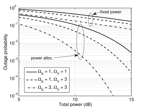
Figure 3: Outage performance improvement due to power allocation

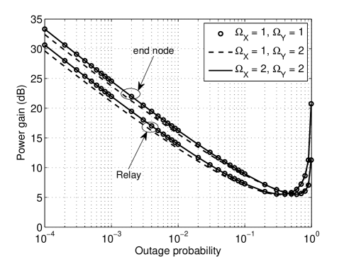
Figure 4: Power savings at the end nodes and the relay

References

• [1] B. Rankov and A. Wittneben, ”Spectral Efficient Protocols for Half-Duplex Fading Relay Channels”, IEEE J. Sel. Areas Commun., vol. 25, no. 2, pp. 379–389, Feb. 2007
• [2] T. J. Oechtering, C. Schnurr, I. Bjelakovic, and H. Boche, ”Broadcast Capacity Region of Two-Phase Bidirectional Relaying”, IEEE Trans. Info. Theory, vol. 54, no. 1, pp. 454-458, Jan. 2008
• [3] S.-Y. R. Li, R. W. Yeung, and N. Cai, ”Linear Network Coding”, IEEE Trans. Inf. Theory, vol. 49, no. 2, pp. 1204–1216, Feb. 2003
• [4] S. J. Kim, P. Mitran, and V. Tarokh, ”Performance Bounds for Bidirectional Coded Cooperation Protocols”, IEEE Trans. Info. Theory, vol. 54, No. 11, pp. 5235-5241, Nov. 2008
• [5] S. J. Kim, P. Mitran, C. John, R. Ghanadan, and V. Tarokh, β€œCoded Bi-directional Relaying in Combat Scenarios”,Β Proc. IEEE MILCOM 2007, pp. 1–7, Oct. 2007
• [6] P. Liu, and I.-M. Kim, ”Performance Analysis of Bidirectional Communication Protocols Based on Decode-and-Forward Relaying”, IEEE Trans. on Commun., vol. 58, no. 9, pp. 2683-2697, Sept. 2010
• [7] N. Ahmed, M. A. Khojastepour, A. Sabharwal, and B. Aazhang, ”Outage Minimization with Limited Feedback for the Fading Relay Channel”, IEEE Trans. on Commun., vol. 54, no. 4, Apr. 2006
• [8] D. Gunduz, and E. Erkip, ”Opportunistic Cooperation by Dynamic Resource Allocation”, IEEE Trans. Wireless Commun., vol. 6, no. 4, pp. 1446-1454, Apr. 2007
• [9] A. J. Goldsmith and P. Varaiya, β€œCapacity of Fading Channels with Channel Side Information”, IEEE Trans. Info. Theory, vol. 43, no. 6, pp. 1986-1992, Nov. 1997
• [10] G. Caire, G. Taricco, and E. Biglieri, ”Optimum Power Control over Fading Channels”, IEEE Trans. Info. Theory, vol. 45, no. 5, pp. 1468-1489, July 1999
• [11] M. Abramowitz and I.A. Stegun, Handbook of Mathematical Functions with Formulas, Graphs, and Mathematical Tables, 9th Ed. Dover, 1970