An Overview of the Anomalous Soft Photons in Hadron Production

Abstract:

Productions of soft photon with low transverse momenta in high-energy hadron-hadron collisions and $e^{+}$-$e^{-}$ annihilations indicate that they are consistently produced in excess of what are predicted by electromagnetic bremsstrahlung when hadrons (mostly mesons) are produced, but they agree with electromagnetic bremsstrahlung predictions in the absence of hadron production. These excess soft photons are called anomalous soft photons. The occurrence of anomalous soft photons in association with hadron production reveals the presence of additional QED soft photon sources in QCD hadron production. Many different models have been proposed to explain the anomalous soft production. We shall examine specifically a quantum field theory of simultaneous meson and soft photon production in QCD$\times$QED in which the meson production arises from the oscillation of color charge densities of the quarks of the underlying vacuum in a flux tube. As a quark carries both a color charge and an electric charge, the oscillation of the color charge densities will be accompanied by the oscillation of electric charge densities, which will in turn lead to the simultaneous production of anomalous soft photons during the meson production process.

1 Introduction

In many exclusive measurements in the production of hadrons (mostly mesons) since the 1980’s [1]-[10], it was found that the production of associated soft photons with transverse momenta of many tens of MeV is consistently greater than what is predicted from the Low Theorem [11] of electromagnetic bremsstrahlung. The excess low-$k_{T}$ soft photons are called anomalous soft photons. They have been observed in high-energy $K^{+}p$ [1, 2], $\pi^{+}p$ [2], $\pi^{-}p$ [3, 4, 5], $pp$ collisions [6], and $e^{+}$-$e^{-}$ annihilations in $Z^{0}$ hadronic decay [7]-[10]. They are absence when hadrons are not produced [7].

Theoretical treatment of the anomalous soft photons associated with hadron production is a difficult problem because it involves the hadron production in QCD, the soft photon production in QED, and the interplay between QCD and QED particle production processes. The occurrence of anomalous soft photons in association with hadron production reveals the presence of additional QED soft photon sources in QCD hadron production. As a definitive quantum theory of hadron production is not yet at hand, the anomalous soft photon problem provide an interesting window to examine non-perturbative aspects of QCD and QED particle production processes.

While many different theoretical models have been proposed to explain the anomalous soft photons, a complete understanding is still lacking. It is of interest to present an overview of the experimental data as well as theoretical approaches in our efforts to comprehend the phenomenon.

2 The Low Theorem

Because the Low Theorem [11] plays an important role in quantifying the excess of soft photon production, it is worthwhile to review its theoretical foundation and its contents.

We consider the process $p_{1}+p_{2}\to p_{3}+p_{4}+k$ where $p_{i}$ represents a hadron and its momentum, and $k$ represents a photon and its momentum. For the simplest case with neutral $p_{2}$ and $p_{4}$, and charged $p_{1}$ and $p_{3}$ hadrons, the Feynman diagrams are shown in Fig. 1. The amplitude for the production of a photon with a polarization $\epsilon$ is

Figure 1: Feynman diagrams                                                                                                 
for $p_{1}$+$p_{2}$$\to$$p_{3}$+$p_{4}$+$k$.                                                                        

$$M(p_{1}p_{2};p_{3}p_{4}k) = M_{0}(p_{1}p_{2};p_{3}p_{4})\left(\frac{e_{1}p_{1}\cdot\epsilon}{(p_{1}-k)^{2}}+\frac{e_{3}p_{3}\cdot\epsilon}{(p_{3}+k)^{2}}\right)~{}~{}~{}~{}~{}~{}~{}$$ (1)

$$=M_{0}(p_{1}p_{2};p_{3}p_{4})\left(\sum_{i}^{\rm all~{}charged~{}particles}\frac{\eta_{i}e_{i}p_{i}\cdot\epsilon}{2p_{i}\cdot k}\right)\!,$$

where $e_{i}$ is the charge of $p_{i}$, and $\eta_{i}$ is +1 for an outgoing hadron and -1 for an incoming hadron respectively. In obtaining the above equation, we have assumed

$$M_{0}(p_{1}-k~{}~{}p_{2};~{}p_{3}~{}p_{4})\sim M_{0}(p_{1}~{}p_{2};~{}p_{3}+k~{}~{}p_{4})\sim M_{0}(p_{1}~{}p_{2};~{}p_{3}~{}p_{4}).$$ (2)

This is a reasonable assumption in high energy processes in which $|{\bf p_{1}}|$ and $|{\bf p_{3}}|$ in the C.M. frame are much greater than the transverse momentum of the soft photon, $k_{T}$. The amplitude $M_{0}$ with the production of a soft photon is then approximately independent of $k$ and can be adequately represented by $M_{0}(p_{1}p_{2};p_{3}p_{4})$, the Feynman amplitude for the production of only hadrons. We can generalize the above Eq. (1) to the process $p_{1}+p_{2}\to p_{3}+p_{4}+...+p_{N}+k$ where $p_{i}$ is a hadron and $k$ is a soft photon. The Feynman amplitude is

$$M(p_{1}p_{2};p_{3}p_{4}...p_{N}k) = M_{0}(p_{1}p_{2};p_{3}p_{4}...p_{N})\left(\sum_{i}^{\rm all~{}charged~{}particles}\frac{\eta_{i}e_{i}p_{i}\cdot\epsilon}{2p_{i}\cdot k}\right),$$ (3)

From the relation between Feynman amplitudes and cross sections, the above equation gives [11]

$$\frac{dN_{\gamma}}{d^{3}k}=\frac{\alpha}{2\pi k_{0}}\int d^{3}p_{1}d^{3}p_{2}d^{3}p_{3}...d^{3}p_{N}\sum_{i,j=1}^{N}\eta_{i}\eta_{j}e_{i}e_{j}\frac{-(p_{i}\cdot p_{j})}{(p_{i}\cdot k)(p_{j}\cdot k)}\frac{dN_{\rm hadrons}}{d^{3}p_{1}d^{3}p_{2}d^{3}p_{3}...d^{3}p_{N}}.$$ (4)

Thus, the spectrum of soft photons can be calculated from exclusive measurements on the spectrum of the produced hadrons.

3 Experimental Measurements of Anomalous Soft Photon in Hadron production

In which part of the photon spectrum are soft photons expected to be important? Upon choosing the beam direction as the longitudinal axis, Eq. (4) indicates that the contributions are greatest when the transverse momentum of the photon, $k_{T}$, is small [12].

Table 1: The ratio of the soft photon yield associated with hadron production to the bremsstrahlung yield in high-energy hadron-hadron collisions and $e^{+}$-$e^{-}$ annihilations, compiled by V. Perepelitsa [9].

Experiment	Collision	Photon $k_{T}$	Photon/Brem
	Energy		Ratio
$K^{+}p$, CERN,WA27, BEBC (1984)	70 GeV/c	$k_{T}<$ 60 MeV/c	4.0 $\pm$0.8
$K^{+}p$, CERN,NA22, EHS (1993)	250 GeV/c	$k_{T}<$ 40 MeV/c	6.4 $\pm$1.6
$\pi^{+}p$, CERN,NA22, EHS (1997)	250 GeV/c	$k_{T}<$ 40 MeV/c	6.9 $\pm$1.3
$\pi^{-}p$, CERN,WA83,OMEGA (1997)	280 GeV/c	$k_{T}<$ 10 MeV/c	7.9 $\pm$1.4
$\pi^{+}p$, CERN,WA91,OMEGA (2002)	280 GeV/c	$k_{T}<$20 MeV/c	5.3 $\pm$0.9
$pp$, CERN,WA102,OMEGA (2002)	450 GeV/c	$k_{T}<$20 MeV/c	4.1 $\pm$0.8
$e^{+}$$e^{-}$$\to$hadrons, CERN,DELPHI	$\sim$91 GeV(CM)	$k_{T}<$60 MeV/c	4.0
with hadron production (2010)
$e^{+}$$e^{-}$$\to$$\mu^{+}$$\mu^{-}$, CERN,DELPHI	$\sim$91 GeV(CM)	$k_{T}<$60 MeV/c	1.0
with no hadron production (2008)

Many high-energy experiments were carried out to measure the spectrum of photons with transverse momenta of the order of many tens of MeV. The soft photon yields are then compared with what are expected from electromagnetic bremsstrahlung of the hadrons as given by Eq. (4). The results are summarized by Perepelitsa in Table I [9] and reviewed in the comprehensive report in [10]. The experimental measurements indicate that low-$k_{T}$ soft photons are produced in excess of what is expected from the electromagnetic bremsstrahlung process. In particular, in DELPHI measurements in high-energy $e^{+}$-$e^{-}$ annihilations in $Z^{0}$ hadronic decay, the ratio of the soft photon yield to the bremsstrahlung yield associated with hadron production is about 4 [10], whereas the ratio of soft photon yield to the bremsstrahlung yield in the corresponding $e^{+}+e^{-}\to\mu^{+}+\mu^{-}$ reaction is about 1 [7]. This indicates clearly that anomalous soft photons are present only when hadrons are produced.

4 Recent DELPHI Anomalous Soft Photon Data

In addition to measuring the overall ratio of soft photon production, the DELPHI Collaboration carried out measurements of soft photon yields in different phase space in coincidence with various hadron production variables. They provide a wealth of information on the characteristics of the produced hadrons associated with the anomalous soft photons [7]-[10]. The main features of the observations from the DELPHI Collaboration can be summarized as follows:

1. Anomalous soft photons are produced in association with hadron production at high energies. They are absent when there is no hadron production [8].

2. The anomalous soft photon yield is proportional to the hadron yield.

3. The transverse momenta of the anomalous soft photons are in the region of many tens of MeV/c.

4. The anomalous soft photon yield increases approximately linearly with the number of produced neutral or charged particles, but, the anomalous soft photon yields increases much faster with increasing neutral particle multiplicity than with charged particle multiplicity, as shown in Fig. 2.

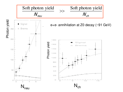
Figure 2: Number of soft photons $N_{\gamma}$ as a function of neutral hadron multiplicity $N_{\rm neu}$ and charged hadron multiplicities $N_{\rm ch}$ from the DELPHI Collaboration [10].

5 Models of Anomalous Soft Photon Production

Many different model have been proposed to explain the anomalous soft photon production in association with hadron production. As the transverse momenta of the anomalous photons are of order of many tens of MeV, Van Hove and Lichard suggested that there is a source of these low-energy photons in the form of a glob of cold quark-gluon system of low temperature with $T\sim$10 to 30 MeV at the end of parton virtuality evolution in hadron production [13]. In such a cold quark-gluon plasma, soft photons may be produced by $q+\bar{q}\to\gamma+g$ or $g+q\to\gamma+q$, and will acquire the characteristic temperature of the cold quark-gluon plasma. Kokoulina $et~{}al.$ followed similar idea of a cold quark-gluon plasma as the source of soft photon production [14]. Collaborative evidence of a cold quark-gluon plasma with $T\sim$ 10 to 30 MeV from other sources however remain lacking.

Barshay proposed that pions propagate in pion condensate and they emit soft photons during the propagation. Rate of soft photon emission depends on the square of pion multiplicity [15]. The concept of a pion condensation in high-energy $e^{+}$-$e^{-}$ annihilations in $Z^{0}$ hadronic decay has however not been well established. Shuryak suggested that soft photons are produced by pions reflecting from a boundary under random collisions. Hard reflections lead to no effect, but soft pion collisions on wall leads to large enhancement in soft photon yield [16]. Czyz and Florkowski proposed that soft photons are produced by classical bremsstrahlung, with parton trajectories following string breaking in a string fragmentation. They suggested that photon emissions along the flux tube agree with the Low limit whereas photon emissions perpendicular to the flux tube are enhanced over the Low limit [17]. Nachtmann $et~{}al.$ suggested that soft photons produced by synchrotron radiation from quarks in the stochastic QCD vacuum [18]. Hatta and Ueda suggested that soft photons are produced in ADS/CFT supersymmetric Yang-Mills theory [19]. Simonov suggested that soft photons arose from closed quark-antiquark loop [20].

Wong proposed that soft photons arises in conjunction with the production of hadron in the quantum field theory of particle production in QCD2 and QED2 [21]. Such a mechanism will be discussed in more detail in subsequent sections. Following similar lines of quantum field theory in two-dimensions, Kharzeev and Loshaj suggested that soft photons arises from the induced current in Dirac sea [22].

6 Quantum Field Theory of Simultaneous Meson and Soft Photon Production

While the various proposed models may explain some features of the soft photon production process, the fourth feature listed in Section 4 from recent DELPHI observations cannot be explained by almost all existing models [9, 10]. As the DELPHI data reveals differential properties associated with the charged and neutral hadron multiplicities and these multiplicities depend on the isospin properties of the produced hadrons, we seek a quantum field theory description for the simultaneous production of hadrons and anomalous soft photons with explicit flavor degrees of freedom in $q$-$\bar{q}$ string-fragmentation that may explain this peculiar feature of the phenomenon [21].

As described by Casher, Kogut, and Suskind [23], the meson production in the quantum field theory arises from the oscillation of color charge densities of the quark vacuum in the flux tube when a quark and an antiquark (or a diquark) pull away from each other at high energies. The meson rapidity distribution of these produced exhibits a rapidity plateau, whose width increases with energy as $\ln(\sqrt{s})$. These color charge density oscillations obey Klein-Gordon equations characterized by different masses of the mesons [23]-[34]. Because a quark carries both a color charge and an electric charge, the underlying dynamical motion of the quarks in the vacuum that generate color charge density oscillations will also generate electric charge density oscillations in the flux tube. These color charge density oscillations will lead to the production of photons that are additional to those from the electromagnetic bremsstrahlung process. Thus the oscillation of the quark densities in the vacuum will lead to the simultaneous color and electric charge density oscillations and will subsequently lead to simultaneous and proportional production of mesons and anomalous photons in the flux tube, in agreement with the first two features of the anomalous soft photon phenomenon listed in Section 4.

It is of interest to examine whether the model also leads to results that will be consistent with the other features of the anomalous soft photon production phenomenon listed in Section 4. For such a purpose, we study quarks interacting with both QCD and QED interactions in the U$(3)$ group which comprises of the QCD color SU(3) and the QED electromagnetic U(1) subgroups with different coupling constants. We introduce the generator $t^{0}$ for the U$(1)$ subgroup,

$$t^{0}=\frac{1}{\sqrt{6}}\left(\matrix{1&0&0\cr 0&1&0\cr 0&0&1}\right),$$ (5)

which adds on to the eight generators of the SU$(3)$ subgroup, $\{t^{1},...t^{8}\}$, to form the nine generators of the U(3) group. They satisfy ${\rm tr}\{t^{\alpha}t^{\beta}\}=\delta^{\alpha\beta}/2{~{}~{}\rm for~{}~{}}\alpha,\beta=0,1,..,8$.

We examine the QCD4$\times$QED4 system with two flavors in four-dimensional space-time $x^{\mu}$. The dynamical variables are the quark fields, $\psi_{f}^{a}$, and the U(3) gauge fields, $A_{\nu}$=$A_{\nu}^{\alpha}t^{\alpha}$, where $a$ is the color index, $f$ the flavor index, and $\alpha$ the U(3) generator index with coupling constants $g_{f}^{\alpha}$,

$$g_{u}^{\{1,..,8\}}=g_{d}^{\{1,..,8\}}=g_{\rm QCD4},{\rm~{}~{}for~{}~{}QCD},$$ (6)

$$g_{u}^{0}=-e_{u}=-Q_{u}e_{\rm QED4},~{}~{}~{}g_{d}^{0}=-e_{d}=-Q_{d}e_{\rm QED4},~{}~{}~{}Q_{u}=2/3,~{}~{}~{}Q_{d}=-1/3{\rm~{}~{}for~{}~{}QED}.$$ (7)

The transverse confinement of the flux tube can be represented by quarks moving in a transverse scalar field $m({\bf r})$ where $m({\bf r})=S({\bf r})$+(current quark mass $m_{q}$) and $S({\bf r})$ is the confining scalar interaction arising from nonperturbative QCD. The equation of motion of the quark field $\psi$ is

$$\left\{iD\!\!\!\!/-m({\bf r})\right\}\psi=0,$$ (8)

where

$$iD\!\!\!\!/=\gamma^{\mu}\Pi_{\mu}=\gamma^{\mu}(p_{\mu}+gA_{\mu}).$$ (9)

The equation of motion for the gauge field $A_{\mu}$ is

$$D_{\mu}F^{\mu\nu}=\partial_{\mu}F^{\mu\nu}-ig[A_{\mu},F^{\mu\nu}]=gj^{\nu},$$ (10)

where

$$F_{\mu\nu}=\partial_{\mu}A_{\nu}-\partial_{\nu}A_{\mu}-ig[A_{\mu},A_{\nu}],$$ (11)

$$F_{\mu\nu}=F_{\mu\nu}^{\alpha}t^{\alpha},~{}~{}~{}j^{\nu}=j_{f}^{\nu\,\alpha}t^{\alpha},$$ (12)

$$j^{\nu\,\alpha}=2~{}{\rm tr}~{}{\bar{\psi}}_{f}\gamma^{\nu}t^{\alpha}\psi_{f}.$$ (13)

Because of the commutative properties of the $t^{0}$ generator, the commutator terms in Eqs. (10) and (11) give zero contributions for QED.

In the problem of particle production at high energies, the momentum scales for longitudinal dynamical motion of the leading $q$ and $\bar{q}$ as well as those of quarks in the underlying vacuum are much greater than the momentum scales for their transverse motion. Hence, inside the flux tube, $A^{1}$ and $A^{2}$ can be approximately neglected and $A^{0}$ and $A^{3}$ can be considered as a function of $(x^{0},x^{3})$ only. Under the longitudinal dominance and transverse confinement, the QCD4$\times$QED4 system can be approximate compactified as a QCD2$\times$QED2 system with a quark transverse mass $m_{T}$, and the flux tube can be idealized as a $q$-$\bar{q}$ string [33]. The coupling constant in two-dimensional space-time $g_{\rm 2D}$ and four-dimensional space-time $g_{\rm 4D}$ are approximately related by [33]

$$g_{\rm 2D}^{2}\sim\frac{g_{\rm 4D}^{2}}{\pi R_{T}^{2}}.$$ (14)

A formal formulation of the compactification in a flux tube can be carried out using the action integral, with a more rigorous definition of the coupling constant normalization [35].

7 Bosonization of QCD2$\times$QED2 for quarks with two flavors

Subsequent to the compactification, we can work with the effective theory of QCD2$\times$QED2 in two-dimensional space-time. For brevity of notation, the two-dimensional nature of various quantities will be understood in what follows except specified otherwise. The Lagrangian density for QCD2$\times$QED2 that corresponds to the two-dimensional version of Eqs. (8)-(13) is

$${\cal L}={\bar{\psi}}[\gamma^{\mu}(i\partial_{\mu}+gA_{\mu})-m_{T}]\psi-\frac{1}{4}F_{\mu\nu}F^{\mu\nu}.$$ (15)

To search for bound states arising from the density oscillations of the color and electric quark charges in QCD2$\times$QED2, one can use the method of bosonization in which bi-linear products of fermion field variables can be represented by functions of boson field variables. The bosons are bound and nearly free, with residual sine-Gordon interactions that depend on the quark mass [27, 28],[36]-[42]. The bosonization program consists of introducing boson fields to describe an element $u$ of the U(3) group and showing subsequently that these boson fields lead to stable bosons with finite or zero masses.

For the QED2 bosonization in electromagnetic U(1), an element of the U(1) subgroup can be represented by the boson field $\phi^{0}$ as $u=\exp\{i2\sqrt{\pi}\phi^{0}t^{0}\}$. Such a bosonization poses no problem as it is an Abelian bosonization. It will lead to a stable boson as in Schwinger’s QED2 [25].

For the QCD2 bosonization in color SU(3), we need to introduce boson fields to describe an element $u$ of SU(3) in terms of the eight $t^{\alpha}$ generators, as represented in general by $u=\exp\{i2\sqrt{\pi}\phi\sum_{\alpha=1}^{8}n^{\alpha}t^{\alpha}\}$ with an amplitude $\phi$ and the unit vector ${\bf n}$=$\{n^{1},n^{2},..,n^{8}\}$. The bosonization of the fermion current depends on $u^{-1}$ and $\delta u/\delta x^{\pm}$ [38]. A variation of $\delta u/\delta x^{\pm}$ in any of the seven orientation angles of ${\bf n}$ will lead to $\delta u/\delta x^{\pm}$ quantities along other $t^{\alpha}$ directions. These variations of $\delta u/\delta x^{\pm}$ will not in general commute with $u$ or $u^{-1}$. They will lead to $j_{\pm}$ currents that are complicated non-linear functions of the eight generator degrees of freedom and will make it difficult to look for stable boson states with these currents. On the other hand, a variation of the amplitude $\phi$ in $u$, with the orientation of ${\bf n}$ held fixed, will lead to $\delta u/\delta x^{\pm}$ that commutes with $u$ and $u^{-1}$ in the bosonization formula, as in the Abelian case. It will lead to simple currents and stable QCD2 bosons with well defined masses. We are therefore well advised to search for stable bosons by varying only the amplitude of $\phi$, keeping the orientation of ${\bf n}$ fixed. As a unit vector ${\bf n}$ in any orientation can be rotated to the first axis along the $t^{1}$ direction by an orthogonal transformation in the $\alpha$-space, we can consider the unit vector ${\bf n}$ to lie along the $t^{1}$ direction for the bosonization of the color SU(3) subgroup. We are therefore justified to bosonize an element $u$ of the U(3) group as

$$u=\exp\{i2\sqrt{\pi}\sum_{\alpha=0}^{1}\phi^{\alpha}t^{\alpha}\}.$$ (16)

With such a bosonization, the kinetic energy, the interaction energy, and the mass term lead to the Hamiltonian density [21]

$${\cal H} = \frac{1}{2}N_{\mu}\sum_{\alpha=0}^{1}\biggl{\{}\sum_{f=u,d}\left[\frac{1}{2}(\Pi_{f}^{\alpha})^{2}+\frac{1}{2}(\partial_{1}\phi_{f}^{\alpha})^{2}\right]+\frac{1}{2\pi}(\sum_{f=u,d}g_{f}^{\alpha}\phi_{f}^{\alpha})^{2}\biggr{\}}$$ (17)

$$-\frac{e^{\gamma}m_{T}\mu}{2\pi}2N_{\mu}\sum_{f=u,d}\cos(2\sqrt{\pi/6}\phi_{f}^{0})\cos(2\sqrt{\pi/4}\phi_{f}^{1}),$$

where for $N_{\mu}$ is the normal order operator for the mass scale $\mu$ [28, 37].

In the flavor sector, the up and down quarks combine to form the isoscalar $(I,I_{3})$=$(0,0)$ and the isovector $(I,I_{3})$=(1,1), (1,0), (1,-1) states. The $(I,I_{3})$=$(1,\pm 1)$ QED2 states involve composite constituents with like electric charges and are unlikely to be stable in the electromagnetic sector. We shall therefore focus our attention only on the QED2 neutral isoscalar boson ($I$=0,$I_{3}$=0) and neutral isovector boson ($I$=1,$I_{3}$=0) states. In QCD with two flavors, there is an approximate isospin symmetry, and the QCD quark-antiquark meson states have isospin quantum numbers $I$ with nearly degenerate $2I$+1 $I_{3}$-components.

We can construct the $\phi_{I}^{\alpha}$ fields for the isospin $(I,I_{3}=0)$ states, for up and down quark fields moving in phase or out of phase,

$$\phi_{I}^{\alpha}=\frac{1}{\sqrt{2}}\left[\phi_{u}^{\alpha}+(-1)^{I}\phi_{d}^{\alpha}\right]~{}~{}{\rm and}~{}~{}~{}\Pi_{I}^{\alpha}=\frac{1}{\sqrt{2}}\left[\Pi_{u}^{\alpha}+(-1)^{I}\Pi_{d}^{\alpha}\right].$$ (18)

The Hamiltonian density for boson fields of different isospin quantum numbers $I$ and $I_{3}=0$ is

$${\cal H}=\frac{1}{2}N_{\mu}\biggl{\{}\sum_{\alpha=0}^{1}\sum_{I=0}^{1}\biggl{[}\frac{1}{2}(\Pi_{I}^{\alpha})^{2}+\frac{1}{2}(\partial_{1}\phi_{I}^{\alpha})^{2}\biggr{]}+V(\{\phi_{I}^{\alpha}\})\biggr{\}},$$ (19)

where $V(\{\phi_{I}^{\alpha}\})=V_{\rm int}(\{\phi_{I}^{\alpha}\})+V_{\rm m}(\{\phi_{I}^{\alpha}\})$ with the interaction energy

$$V_{\rm int}(\{\phi_{I}^{\alpha}\})=\frac{1}{2}\left(\sum_{I=0}^{1}\frac{g_{u}^{\alpha}+(-1)^{I}g_{d}^{\alpha}}{\sqrt{2}\pi}\phi_{0}^{\alpha}\right)^{2},$$ (20)

and the quark mass term

$$V_{\rm m}(\{\phi_{I}^{\alpha}\})=-\frac{e^{\gamma}m_{T}\mu}{2\pi}2\left[\prod_{I=0}^{1}\cos\left(\sqrt{2\pi}(\frac{\phi_{I}^{0}}{\sqrt{6}}+\frac{\phi_{I}^{1}}{\sqrt{4}})\right)+\prod_{I=0}^{1}\cos\left(\sqrt{2\pi}(\frac{\phi_{I}^{0}}{\sqrt{6}}-\frac{\phi_{I}^{1}}{\sqrt{4}})\right)\right].$$ (21)

The Hamiltonian density (19) represents a QCD2 and QED2 system of isoscalar and isovector boson fields $\phi_{I}^{\alpha}$ whose field quanta acquire the mass $M_{I({\rm 2D})}^{\alpha}$, which can be evaluated as the second derivatives of the potential at the potential minimum located at $\phi_{0}^{\alpha}=0$ and $\phi_{1}^{\alpha}=0$. We obtain the mass square $(M_{I({\rm 2D})}^{\alpha})^{2}$ of stable boson quanta

$$(M_{I({\rm 2D})}^{\alpha})^{2}=\biggl{[}\frac{\partial^{2}}{\partial(\phi_{I}^{\alpha})^{2}}V(\{\phi_{I}^{\alpha}\})\biggr{]}_{\phi_{0}^{\alpha},\phi_{1}^{\alpha}=0}=\left(\frac{g_{u}^{\alpha}+(-1)^{I}g_{d}^{\alpha}}{\sqrt{2\pi}}\right)^{2}+\frac{2}{3-\alpha}e^{\gamma}m_{T}\mu,$$ (22)

where $\alpha=0$ for QED2 and $\alpha=1$ for QCD2. As the boson field $\phi_{I}^{\alpha}$ is related to the $\alpha$-gauge field, the quanta of $\phi_{I}^{\alpha}$ are also the quanta of the $\alpha$-gauge fields. The QCD2 bosons and QED2 bosons can be appropriately called QCD2 mesons and QED2 photons respectively. Because $(M_{I({\rm 2D})}^{\alpha})^{2}\geq 0$, the QCD2 mesons and QED2 photons are stable bosons. The self-consistency of gauge field oscillations and the induced quark density oscillations lead to an equation of motion for the gauge field oscillations in the form of Klein-Gordon equations characterized by the corresponding masses.

If $(m_{T}\mu)$=0 (which corresponds to the massless quark limit), the QCD2$\times$QED2 bosons are free. With a finite value of $(m_{T}\mu)$, they interact with a sine-Gordon residual interaction whose strength depends on $(m_{T}\mu)$.

8 QCD2 Meson and QED2 Photon Masses for Quarks with Two Flavors

Equation (22) gives the QCD2 meson and QED2 photon masses for quarks with two flavors. As given by Eq. (14), the QCD2 and QED2 coupling constants for quarks in a flux tube are

$$g_{\rm QCD2}^{2}\sim\frac{g_{\rm QCD4}^{2}}{\pi R_{T}^{2}}\sim\frac{4\alpha_{s}}{R_{T}^{2}},~{}~{}~{}{\rm and}~{}~{}~{}e_{\rm QED2}^{2}\sim\frac{e_{\rm QED4}^{2}}{\pi R_{T}^{2}}\sim\frac{4\alpha}{R_{T}^{2}},$$ (23)

where $\alpha_{s}=g_{\rm QCD4}^{2}/4\pi$ is the strong interaction coupling constant and $\alpha=e_{\rm QED4}^{2}/4\pi=1/137$ is the fine structure constant. The magnitude of the flux tube radius $R_{T}$ is revealed by the root-mean-squared transverse momentum of produced hadrons (mostly pions) as

$$R_{T}\sim\frac{1}{\sqrt{\langle p_{T}^{2}\rangle_{\pi}}},$$ (24)

which empirically is slightly energy-dependent [34]. We shall focus our attention in high energy $e^{+}$-$e^{-}$ annihilations in the hadronic decay of $Z^{0}$ at $\sqrt{s}\sim$91 GeV for which $\sqrt{\langle p_{T}^{2}\rangle_{\pi}}=0.56$ GeV [43], and thus $R_{T}\sim 0.35$ fm. We can infer the value of the nonperturbative strong coupling constant $g_{\rm QCD2}$ from the string tension coefficient $\kappa\sim 1$ GeV/fm that is related to $g_{\rm QCD2}$ by $g_{\rm QCD2}^{2}=2\kappa$ [32, 33, 34]. We have

$$g_{\rm QCD2}=0.632{\rm~{}GeV}~{}~{}~{}{\rm and}~{}~{}~{}e_{\rm QED2}\sim 0.096{\rm~{}GeV}.$$ (25)

With these coupling constants, ($g_{u}^{1}$=$g_{d}^{1}$=$g_{\rm QCD2}$, $g_{u}^{0}$=$-Q_{u}e_{\rm QED2}$, and $g_{d}^{0}$=$-Q_{d}e_{\rm QED2})$, the QCD2 and QED2 boson masses in the massless quark limit of $(m_{T}\mu)$=0 are shown in Table I. One observes that QCD2 for quarks with two flavors gives a massless pion in the massless quark limit, in agreement with the concept of the pion being a Goldstone boson in the standard QCD theory. The massless isovector QCD2 meson lies lower than the isoscalar QCD2 meson of 504 MeV, whereas the ordering is opposite for the QED2 photons, with an isoscalar QED2 photon at 12.8 MeV and an isovector QED2 photon at 38.4 MeV. These QED2 photons lie in the region of observed anomalous soft photons.

Table 2: QED2 and QCD2 boson masses obtained with $R_{T}$=0.35 fm and $g_{\rm QCD2}^{2}$=$2b$=0.4 GeV².

		QCD2	QED2
Coupling Constant		$g_{\rm QCD2}$=632.5 MeV	$e_{\rm QED2}$=96 MeV
$(m_{T}\mu)$=0	isoscalar boson mass $M_{0({\rm 2D})}$	504.6 MeV	12.8 MeV
	isovector boson mass $M_{1({\rm 2D})}$	0	38.4 MeV
$m_{T}$=400 MeV	isoscalar boson mass $M_{0({\rm 2D})}$	734.6 MeV
$\mu$=$m_{T}$	isovector boson mass $M_{1({\rm 2D})}$	533.8 MeV
$m_{T}$= 400 MeV	isoscalar boson mass $M_{0({\rm 2D})}$		$O$(25.3 MeV)
$\mu$=$m_{q}$=$O$(1 MeV)	isovector boson mass $M_{1({\rm 2D})}$		$O$(44.1 MeV)

Equation (22) indicates that the boson masses depend on four mass scales: $g_{\rm QCD2}$, $e_{\rm QED2}$, $m_{T}$, and $\mu$. Because a pion is a quark-antiquark composite, we can estimate the quark transverse mass $m_{T}$ from the pion transverse momentum, $m_{T}\sim\sqrt{\langle p_{T}^{2}\rangle_{\pi}/2}$ which gives $m_{T}\sim 0.4$ for $Z^{0}$ hadronic decay. The mass scale $\mu$ arises from the bosonization of the scalar density ${\bar{\psi}}\psi$ which diverges in perturbation theory. It has to be renormalized such that $\langle{\bar{\psi}}\psi\rangle$=0 in a free theory. It will need to be renormal-ordered again in an interacting theory [28]. The scalar density and the corresponding mass scale therefore depends on the interaction. For the strong interaction of QCD, confinement and chiral symmetry breaking dominate and lead to a transverse mass $m_{T}$ that is much greater than the current quark mass. It is reasonable to take the mass scale $\mu$ to be the same as the quark transverse mass $m_{T}$ in QCD2. In QED2 with a relatively weak interaction, the scalar density ${\bar{\psi}}\psi$ that diverges in perturbation theory has to be renormalized in a nearly-free field in which the quark energy is just the current quark masses. The mass scale $\mu$ for QED2 should therefore be the QED current quark mass $m_{q}$ appropriate for a nearly-free theory. We shall take $\mu=1$ MeV for QED2.

The values of the QCD2 and QED2 boson masses obtained with these coupling constants and mass scales $\mu$ are given in Table I. They give a QCD2 isovector meson mass of 0.534 GeV and a QCD2 isoscalar meson mass of 0.735 GeV in the flux tube and an isoscalar photon of order 25 MeV and an isovector photon of order 44 MeV. They fall within the same order of magnitude of the transverse masses of produced mesons and anomalous soft photons.

We can infer from the quantum field theory description of particle production in Ref. [23] that the QCD2 mesons and QED2 photons will be produced simultaneously in the same process of $q$-$\bar{q}$ string fragmentation, when a quark pulls away from an interacting antiquark at high energies. The production of a QCD2 meson of a certain isospin quantum number will be accompanied by the production of a QED2 photon of the same isospin, with appropriate probability ratios.

In the emergence of the boson from two-dimensional space-time to four-dimensional space-time, we envisage an adiabatic transverse expansion from the two-dimensional flux tube to the full configuration space. The adiabatic transverse expansion involves no change of the particle energy and particle longitudinal momentum so that the boson mass $M_{I({\rm 2D})}^{\alpha}$ in two-dimensional space-time turns into the boson transverse mass $M_{IT}^{\alpha}$ in four-dimensional space-time. For example, we can consider the production of the lowest-mass isovector meson, which is a pion. Theoretically, Table I gives a produced pion of mass $M_{I=1({\rm 2D})}^{\alpha}$=0.534 GeV in the flux tube, corresponding to a boson of transverse mass 0.534 GeV in four-dimensional space-time. Experimentally, a pion is produced with an average $\sqrt{\langle p_{T}^{2}\rangle}_{\pi}\sim 0.56$ GeV [43] for the $Z^{0}$ hadronic decay and the experimental (average) isovector meson (pion) transverse mass is $M_{1T}^{h}$= 0.579 GeV, which is close to the value of 0.534 GeV in Table I. We consider next the production of the lowest mass isoscalar meson, which is the $\eta$ meson with a rest mass $M_{\eta}=0.547$ GeV. Theoretically, Table I gives a produced isoscalar particle of mass $M_{I=0({\rm 2D})}^{\alpha}$=0.735 GeV in the flux tube, corresponding to a boson of transverse mass 0.735 GeV in four-dimensional space-time. Experimentally, the average transverse momentum of $\eta$ has however not been measured. As the $\eta$ meson has approximately the same mass as a kaon whose average transverse momentum has been measured, the average transverse momentum of the $\eta$ meson should be of the order of the kaon average transverse momentum of $\sqrt{\langle p_{T}^{2}\rangle_{K}}$$\sim$ 0.616 GeV [44]. Upon taking this estimate to be the isoscalar meson average transverse momentum, the experimental (extrapolated) isoscalar meson ($\eta$ meson) average transverse mass is $M_{0T}^{h}$$\sim$ 0.824 MeV which can be compared well with $M_{\eta({\rm QCD2)}}$=0.735 GeV in Table I. In the case of QED photons, the rest mass of the photon is zero in four-dimensional space-time. Hence, the QED2 photon mass in two-dimensional space-time can be identified as the photon transverse momentum in four-dimensional space-time. They fall within the $k_{T}$ regions of anomalous soft photons.

9 Rates of Meson and Anomalous Soft Photon Production

To obtain an estimate on the rate of particle production, we shall use the Schwinger mechanism of particle production in a strong field [45]-[48]. The probability of particle production of a composite particle of transverse mass $M_{IT}^{\alpha}$ in an electric field of strength $\kappa_{q\bar{q}}^{\alpha}$ depends on the exponential factor of $\exp\{-\pi(M_{IT}^{\alpha}/2)^{2}/\kappa_{q\bar{q}}^{\alpha}\}$, where the factor of 1/2 in $M_{IT}^{\alpha}/2$ is to denote the production of a pair of particles each of which has a mass $M_{IT}^{\alpha}/2$, and combining one particle of mass $M_{IT}^{\alpha}/2$ with the neighboring particle of mass $M_{IT}^{\alpha}/2$ leads subsequently to a composite stable boson of mass $M_{IT}^{\alpha}/2+M_{IT}^{\alpha}/2$. Furthermore, from dimensional analysis, we can deduce that the rate of production per space-time volume element $(dz\,dt)$ has the dimension $\kappa_{q\bar{q}}^{\alpha}$. We therefore infer from the Schwinger mechanism that the rate of the production of the number of particle of type $\alpha$, isospin $I$, and mass $M_{IT}^{\alpha}$ due to the presence of the QCD and QED fields between a receding quark $q$ and an antiquark $\bar{q}$ is

$$\frac{dN_{I}^{\alpha}}{dz\,dt}=A\sum_{q\bar{q}}P_{q\bar{q}}~{}\kappa_{q\bar{q}}^{\alpha}~{}\exp\left\{-\frac{\pi(M_{IT}^{\alpha}/2)^{2}}{\kappa_{q\bar{q}}^{\alpha}}\right\},~{}~{}~{}\alpha=\gamma,h,$$ (26)

where $P_{q\bar{q}}$ is the probability for the quark-antiquark source pair to be a $u\bar{u}$ or $d\bar{d}$ pair, and $A$ is a dimensionless constant. In an $e^{+}$-$e^{-}$ annihilation at high energies, there is an equal probability for the quark-antiquark leading source pair to be a $u\bar{u}$ or $d\bar{d}$ pair, and so $P_{u\bar{u}}=P_{d\bar{d}}=1/2$.

For the production of QCD2 mesons, the color electric field strength between the leading quark and antiquark is independent of the quark flavor quantum number. It is given by

$$\kappa_{u\bar{u}}^{h}=\kappa_{d\bar{d}}^{h}={g_{\rm QCD2}^{2}}/{2}=\kappa.$$ (27)

For the production of QED2 photons, the electric field strength between the leading source quark $q$ and antiquark $\bar{q}$ is given in terms of the electric charges of the quark and the antiquark as

$$\kappa_{q\bar{q}}^{\gamma}=|Q_{q}Q_{\bar{q}}|e_{\rm QED2}^{2}/2.$$ (28)

Then the Schwinger mechanism of Eq. (26) gives

$$\frac{N_{I=0}^{h}}{N_{I=1}^{h}}\sim\frac{1}{4},~{}~{}~{}\frac{N_{I=0}^{\gamma}}{N_{I=1}^{\gamma}}\sim\frac{11}{4},~{}~{}~{}$$ (29)

which reveals that as the mass of an isoscalar meson is greater than the mass of an isovector meson, as given in Table I, so isoscalar mesons are much less likely produced than isovector meson (in a particular $I_{3}$ state). On the other hand, the mass of an isoscalar ($I$=0,$I_{3}$=0) photon is less than the mass of an isovector ($I$=1,$I_{3}$=0) photon, so isoscalar photons are much more likely produced than isovector photon. We can also calculate from Eq. (29) the ratio of ratios,

$$\frac{N_{I=0}^{\gamma}}{N_{I=0}^{h}}:\frac{N_{I=1}^{\gamma}}{N_{I=1}^{h}}\sim\frac{11}{4}:\frac{1}{4}=11:1,$$ (30)

which states that the number of soft isoscalar photons associated with the isoscalar meson production are more numerous than soft isovector photons associated with the isovector meson production. The production of an isoscalar $\eta$ meson will lead to 1.64 neutral particles and 0.57 charged particles while the production of an isovector pion will lead, on the average, to 2/3 charged particle and 1/3 neutral particle [49]. Production of an isoscalar meson is associated more with the production of neutral mesons whereas the production of an isovector meson is associated more with the production of charged particles. As a consequence, the above ratio in Eq. (30) suggests that the ratio of the number of soft photons to neutral meson multiplicity is much greater than the ratio of the number of soft photons to charged meson multiplicity, in qualitative agreement with the fourth feature in Section 4 of the DELPHI observation.

10 Conclusions and Discussions

In high energy hadron-hadron collisions and $e^{+}$-$e^{-}$ annihilations, soft photons are produced in excess of what is expected from electromagnetic bremsstrahlung predictions, indicating the presence of additional anomalous QED soft photon production sources in QCD hadron production processes.

We review here various models of anomalous soft photon production. The most intriguing observation from the DELPHI Collaboration is the peculiar feature that the yield of anomalous soft photons increases at a much greater rate with increasing neutral particle multiplicity than with charged particle multiplicity. Such a feature cannot be explained by almost all existing models [9, 10]. We examine in this paper a quantum field theory description of the simultaneous production of hadron and anomalous soft photons in a flux tube that may explain this peculiar feature of the phenomenon [21].

In this description, a color flux tube is formed when a quark and an antiquark (or a diquark) pull apart from each other at high energies. The motion of the quarks in the underlying vacuum of the flux tube generates color charge oscillations which lead to the production of mesons. As a quark carries both a color charge and an electric charge, the color charge oscillations of the quarks in the vacuum are accompanied by electric charge oscillations, which will in turn lead to the simultaneous production of soft photons during the meson production process.

To study these density oscillations, we start with quarks interacting with both QCD and QED interactions in four-dimensional space-time in the U(3) group which breaks into the color SU(3) and the QED U(1) subgroups. Specializing to particle production at high energies, we find that the dominance of the longitudinal motion and transverse confinement lead to the compactification from QED4$\times$QED4 in four-dimensional space-time to QCD2$\times$QED2 in two-dimensional space-time, with the formation of the flux tube. In the flux tube, the self-consistent coupling of quarks and gauge fields lead to color charge and electric charge oscillations that give rise to stable QCD2 bosons and QED2 bosons. The boson masses depend on the gauge field coupling constants. The presence of the flavor degrees of freedom leads to isospin dependence of the boson masses, with the isovector meson mass smaller than the isoscalar meson mass, but the mass ordering is reversed for the isoscalar photon and the isovector photon.

As QCD2 and QED2 bosons are stable in the flux tube environment, we can infer from the quantum field theory description of particle production in Ref. [23] that these QCD2 mesons and QED2 photons will be produced simultaneously in $q$-$\bar{q}$ string fragmentation. Under the condition of adiabaticity with no change of the particle energy and longitudinal momentum after the produced particle emerges from the production region, the boson mass in two-dimensional space-time turns into the boson transverse mass in four-dimensional space-time.

Because both color charge oscillations and electric charge oscillations arise from the same density oscillations of the quarks in the vacuum, both QCD2 meson and QED2 photon will be simultaneously produced by the fragmentation of the $q$-$\bar{q}$ string. As the QCD isoscalar meson mass is greater than the isovector mass, the production of isoscalar mesons is less likely than isovector mesons. In contrast, as the isoscalar photon mass is lower than the isovector photon mass, the production of isoscalar photons is more likely than isovector photons. Production of an isoscalar meson is associated more with the production of neutral mesons whereas the production of an isovector meson is associated more with the production of charged particles. As a consequence, the ratio $N^{\gamma}/N_{\rm neu}$ is much greater than the ratio $N^{\gamma}/N_{\rm ch}$, as observed by the DELPHI Collaboration [9, 10].

While the QCD2$\times$QED2 model appears to explain qualitatively the main features of the experimental anomalous soft photon data, it is desirable to carry out further experimental measurements to test the model:

1. It will be of interest to measure the transverse momentum distribution of the soft photons with a finer $k_{T}$ resolution and greater precision for a given narrow range of photon rapidities. Qualitatively, we expect the production of photons with two different average transverse momenta, one with $\sqrt{\langle k_{T}^{2}\rangle}$ $\sim$ 25 MeV for the production of the isoscalar photon and one with $\sqrt{\langle k_{T}^{2}\rangle}$ $\sim$ 44 MeV for the production of the isovector photon.

2. It will be of interest to measure the transverse momentum distribution by selecting events with predominantly neutral particles and events with predominantly charged particles. The former events will likely arise from the production of isoscalar mesons and QED2 isoscalar photons, with an average photon transverse momentum of $\sim$25 MeV, while the latter from the production of isovector mesons and the isovector photons, with an average photon transverse momentum of $\sim$50 MeV.

3. The rapidity distribution of the produced photons should exhibit the plateau structure, as expected of similar distributions in meson production. A measurement of the rapidity distribution will provide useful additional information on the dynamics of soft photon production.

4. Measurements of the properties of associated hadrons similar to those of the DELPHI Collaboration should be carried out with hadron-hadron collisions at high energies where anomalous soft photon production has been reported [1]-[5].

References

- [1] P.V. Chliapnikov et al., Phys. Lett. B 141, 276 (1984).
- [2] F. Botterweck et al., Z. Phys. C51, 541 (1991).
- [3] S. Banerjee et al., Phys. Lett. B305, 182 (1993).
- [4] A. Belogianni et al.,Phys. Lett. B408, 487 (1997).
- [5] A. Belogianni et al.,Phys. Lett. B548, 129 (2002).
- [6] A. Belogianni et al.,Phys. Lett. B548, 122 (2002).
- [7] J. Abdallah (DELPHI Collaboration), Eur. Phys. J. C47, 273 (2006).
- [8] J. Abdallah (DELPHI Collaboration), Eur. Phys. J. C57, 499 (2008).
- [9] V. Perepelitsa, for the DELPHI Collaboration, Proceedings of the XXXIX International Symposium on Multiparticle Dynamics, Gomel, Belarus, September 4-9, 2009, published in Nonlin. Phenom. Complex Syst. 12, 343 (2009).
- [10] DELPHI Collaboration, J. Abdallah , (DELPHI Collaboration), Eur. Phys. J. C67, 343, (2010).
- [11] F. Low, Phys. Rev. 110, 974 (1958).
- [12] V. N. Gribov, Sov. J. Nucl. Phys. 5, 280 (1967).
- [13] L. Van Hove, Ann. Phys. (N.Y.) 192, 66 (1989); P. Lichard and L. Van Hove, Phys. Lett. B245, 605 (1990); P. Lichard, Phys. Rev. D50, 6824 (1994).
- [14] E. Kokoulina, A. Kutov, V. Nikitin, Braz. J. Phys., 37, 785 (2007); M. Volkov, E. Kokoulina, E. Kuraev, Ukr. J. Phys., 49, 1252 (2003).
- [15] Barshay, Phys. Lett. B227, 279 (1989).
- [16] Shuryak, Phys. Lett. B231, 175 (1989).
- [17] W. Czyz and W. Florkowski, Z. Phys. C61, 171 (1994).
- [18] O. Nachtmann, hep-ph/9411345 G.W. Botz, P. Haberl, O. Nachtmann, Z. Phys. C67, 143 (1995).
- [19] Y. Hatta and T. Ueda, Nucl. Phys. B837, 22 (2010).
- [20] Yu.A. Simonov, Phys. Atom. Nucl., 71, 1049 (2008), hep-ph/07113626; Yu.A. Simonov, JETP Lett., 87, 147 (2008) Yu.A. Simonov, A.I. Veselov, JETP Lett., 88, 79 (2008); Yu.A. Simonov, A.I. Veselov, Phys. Lett. B 671, 55 (2009).
- [21] C. Y. Wong, Phys. Rev. C81, 064903 (2010).
- [22] D. E. Kharzeev and F. Loshaj, arxiv:1308.2716.
- [23] A. Casher, J. Kogut, and L. Susskind, Phys. Rev. D10, 732 (1974).
- [24] J. D. Bjorken, Lectures presented in the 1973 Proceedings of the Summer Institute on Particle Physics, edited by Zipt, SLAC-167 (1973).
- [25] J. Schwinger, Phys. Rev. 128, 2425 (1962); J. Schwinger, in , Trieste Lectures, 1962 (I.A.E.A., Vienna, 1963), p. 89.
- [26] J. H. Lowenstein and J. A. Swieca, Ann. Phys. (N.Y.) 68, 172 (1971).
- [27] S. Coleman, R. Jackiw, and L. Susskind, Ann. Phys. 93, 267 (1975).
- [28] S. Coleman, Ann. Phys. 101, 239 (1976).
- [29] J. D. Bjorken, Phys. Rev. D27, 140 (1983).
- [30] C. Y. Wong, R. C. Wang, and C. C. Shih, Phys. Rev. D44, 257 (1991).
- [31] For a pedagogical discussion of QED2, see Chapter 6 of C. Y. Wong, Introduction to High-Energy Heavy-Ion Collisions, World Scientific Publisher, 1994.
- [32] C. Y. Wong, Phys. Rev. C78, 064905 (2008).
- [33] C. Y. Wong, Phys. Rev. C80, 034908 (2009).
- [34] C. Y. Wong, Phys. Rev. C80, 054917 (2009).
- [35] A. V. Koshelkin and C. Y. Wong, Phy. Rev D 86, 125026 (2012).
- [36] S. Mandelstam, Phys. Rev. D11, 3026 (1975).
- [37] M. B. Halpern, Phys. Rev. D12, 1684 (1975).
- [38] E. Witten, Commun. Math. Phy. 92, 455 (1984)
- [39] D. Gepner, Nucl. Phys. B 252, 481 (1985). J. Phys. A 31, 9925 (1998).
- [40] E. Abdalla, M. C. B. Abdalla, and K. D. Rothe, Two Dimensional Quantum Field Theory, World Scientific Publishing Company, Singapore, 2001.
- [41] Y. Frishman and J. Sonnenschein, Phys. Rep. 223, 309 (1993); Y. Frishmann, A. Hanany, and J. Sonnenschein, Nucl. Phy. B429, 75 (1994); A. Armonic and J. Sonnenschein, Nucl. Phy. B457, 81 (1995); A. Armonic, Y. Frishmann, J. Sonnenschein, and U. Trittmann Nucl. Phy. B537, 503 (1999); A. Abrashikin, Y. Frishmann, and J. Sonnenschein, Nucl. Phy. B703, 320 (2004).
- [42] D. Gross, I. R. Klebanov, A. Matysin, and A. V. Smilga Nucl. Phys. B461, 109 (1996).
- [43] R. Barate (ALPEPH Collaboration), Zeit. Phys. C 74, 451 (1997).
- [44] H. Aihara (TPC/Two_Gamma Collaboration), Lawrence Berkeley Laboratory Report LBL-23737 (1988).
- [45] J. Schwinger, Phys. Rev. 82, 664 (1951).
- [46] R. C. Wang and C. Y. Wong, Phys. Rev. D38, 348 (1988).
- [47] For a pedagogical discussion of Schwinger particle production mechanism, see Chapter 5 of C. Y. Wong, Introduction to High-Energy Heavy-Ion Collisions, World Scientific Publisher, 1994.
- [48] C. Y. Wong, R. C. Wang, and J. S. Wu, Phys. Rev. D51, 3940 (1995).
- [49] C. Amsler (Particle Data Group), Phys. Lett B667, 1 (2008).