Nilsson-SU3 selfconsistency in heavy N=Z nuclei

Abstract

It is argued that there exist natural shell model spaces optimally adapted to the operation of two variants of Elliott’s SU3 symmetry that provide accurate predictions of quadrupole moments of deformed states. A selfconsistent Nilsson-like calculation describes the competition between the realistic quadrupole force and the central field, indicating a remarkable stability of the quadrupole moments—which remain close to their quasi and pseudo SU3 values—as the single particle splittings increase. A detailed study of the $N=Z$ even nuclei from ⁵⁶Ni to ⁹⁶Cd reveals that the region of prolate deformation is bounded by a pair of transitional nuclei ⁷²Kr and ⁸⁴Mo in which prolate ground state bands are predicted to dominate, though coexisting with oblate ones.

I Introduction

Large Scale Shell Model calculations (LSSM), when doable, are the spectroscopic tool of choice in theoretical nuclear structure. When they are not doable it is often advised to switch to other—basically mean field—methods. A common feature of these approaches is the reliance on quadrupole degrees of freedom as the backbone of nuclear structure, which in shell model language translates as dominance of the quadrupole force, which is indeed (or should be) a classic view. Our task is to find ways to put to good use this dominance. It starts by discovering which are the model spaces in which to operate. The choice turns out to be quite unique (the EEI spaces to be defined soon). Though most often it leads to intractably large diagonalizations, it also happens to be tailored to take full advantage of two variants—pseudo and quasi-SU3—of Elliott’s SU3 symmetry su3 . After explaining in detail how these symmetries operate we turn to quantitative estimates of their reliability by defining and implementing a selfconsistent Nilsson nilsson approach in which the interplay of a realistic quadrupole interaction with the spherical central field establishes the resilience of the predicted quadrupole moments. The controlling parameters are the quadrupole moments themselves which in the absence of a central field reduce to one of their SU3-like guises.

These ideas are applied to the heavy even $N=Z$ nuclei shedding light on the hitherto poorly understood competition between prolate and oblate quadrupole coherence. In this region the full interplay of quasi and pseudo SU3 schemes operates, illustrating what will become the rule for well deformed nuclei—so far only schematically explored at the onset of rotational motion at $N=90$ zrpc .

II The natural ZBM (or EEI) model spaces

The usual lore about shell model spaces is that for light and medium nuclei they involve one major oscillator (HO) shell bounded by magic numbers at $N,Z$=4, 8, 20 and 40 while for heavier systems the spin-orbit (SO) force takes over and the magic boundaries move to $N,Z$= 28, 50, 82 and 126. This view has some merit but misses two crucial points: a) the observed shell evolution is not driven by the SO terms present in the NN interactions, but by three body forces (a word on this later); b) the correct model spaces are larger than those defined by the SO boundaries. Let us examine the possible examples.

In the $p$ shell starting at ⁴He, as particles are added the largest orbit $p_{3/2}$ is “Extruded” (or Ejected or Expelled) from the space by becoming a “closed shell” when filled, while the largest orbit in the next shell “Intrudes” so as to define the first of the EI spaces $p_{1/2}d_{5/2}\equiv r_{1}d$ (closing at ²⁸Si). The notation $r_{p}$ stands for “rest of the major shell of principal quantum number $p$” i.e., all the orbits except the largest one. What we miss here is that the $d_{5/2}$ intruder does not come alone but with an $s_{1/2}$ partner, as made evident by the spectrum of ¹³C ensdf . Therefore the correct space is the first of the Extended EI spaces: $r_{1}ds$ (EEI1 or ZBM zbm ), with $ds=d_{5/2}s_{1/2}$; which is the first instance of a “$\Delta j=2$” sequence.

Notation. The full harmonic oscillator shells are called $sd,\,pf,\,sdg$…while the reverse order $ds,\,fp,\,gds$…will be used for the $\Delta j=2$ sequences.

Next candidate comes from the $sd$ shell starting at ¹⁶O where, as it fills, $d_{5/2}$ is separated from its partners while drawing down the largest orbit in the next shell so as to define the EI2 space: $s_{1/2}d_{3/2}f_{7/2}\equiv r_{2}f$ (starting at ²⁸Si and closing at ⁵⁶Ni). Except that we miss again that the intruder comes with its $\Delta j=2$ partner (as seen in ²⁹Si ensdf ) so $r_{2}f$ becomes $r_{2}fp$ (EEI2 or ZBM2) with $fp=f_{7/2}p_{3/2}$. Then we find the space, relevant for this study, $p_{1/2}p_{3/2}f_{5/2}g_{9/2}\equiv r_{3}g$ (EI3 closing at ¹⁰⁰Sn) which is expected to become $r_{3}gds$ (EEI3 or ZBM3) with $gds=g_{9/2}d_{5/2}s_{1/2}$. Direct experimental evidence of the presence of the $\Delta j=2$ partners is hard to obtain in this region, but abundant indirect evidence will be presented in this paper.

Digression on shell formation. One objection to the description above is that ¹²C and ²⁸Si are not closed shells (though ⁵⁶Ni is, to a good approximation). However EI numbers at $N,Z$=6, 14, 28, 50, 82 and 126 provide good boundaries and many convincing candidates to magicity in the light nuclei (such as ¹⁴C, ²²O and ³⁴Si) and the only systematic magic numbers beyond. The transition from HO to EI major closures demands three-body mechanisms whose irrefutable need is now established on theoretic abin3b and empiric zu3b ; dz10 grounds. Explicit introduction of three-body forces ot3b does not lead so far to consistent agreement with the empirical results. The (hard to sell) notation EI instead of the usual SO is meant to stress that the spin orbit force—in the classic $l\cdot s$ sense—is perfectly given by existing NN interactions above HO closures where it is responsible for the largest orbit coming lowest sz . However, it is definitely not responsible for the EI closures which demand splittings much larger that the $l\cdot s$ one provided by the NN interactions. To fix ideas: in ⁴⁸Ca they would produce a $f_{7/2}-p_{3/2}$ single particle gap equal to that in ⁴¹Ca i.e., 2.5 MeV smaller than the observed one. A discrepancy that increases to some 4.5 MeV in ⁵⁶Ni. The evolution of subshell SO ordering on top of HO closures to the EEI patterns is illustrated in Fig. 1 for different model spaces.

Figure 1: (color online) Evolution of model spaces from Spin-orbit (SO) (around HO closures) to Extended Extruder-Intruder (EEI) made of Pseudo-SU3 and Quasi-SU3 subspaces (explained in Section III).

Both $r_{1}ds$ (ZBM) and $r_{2}fp$ (ZBM2 or SDFP) models lead to feasible and successful diagonalizations in the neighborhood of ¹⁶O and ⁴⁰Ca zbm ; rmp . The $r_{3}gds$ space is expected to work equally well around ⁸⁰Zr—formally the magic upper boundary of the $pf$ shell—which turns out to be a splendid rotor lister . A pure $pf$ description starts failing around $N,Z\approx 34$, and it could be hoped that $r_{3}g$ would cope beyond, but the calculations (always feasible though sometimes hard) fail to produce strongly deformed prolate bands demanded by the data. Which are naturally explained in the $r_{3}gds$ space as we shall demonstrate notwithstanding the near impossibility of exact diagonalizations: First through heuristic arguments based on the approximate SU3 symmetries, and then by very simple selfconsistent calculations that account semi quantitatively for the interplay between the realistic quadrupole interaction and the monopole central field.

III Quadrupole coherence: SU3, pseudo-SU3 and quasi-SU3

Nuclear rotational motion was predicted by Bohr and Mottelson in 1953 bm53 . The idea was that nuclei could acquire a permanent quadrupole deformation in their intrinsic frame, that would translate into a $J(J+1)$ spectrum in the laboratory frame. Historically, this first example of spontaneously broken symmetry was confronted with the need to explain how a deformed intrinsic state—which has no definite angular momentum $J$—could be an eigenstate of a system that must necessarily conserve $J$. The elegant way out was found by Elliott whose SU3 model su3 provides a rigorous example of intrinsic states that are not eigenstates of a Hamiltonian $H$ but of $H-\lambda J(J+1)$.

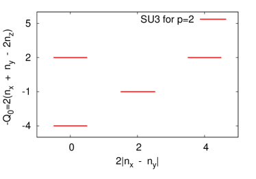
Figure 2: (color online) Eigenstates of $-2q_{20}$. SU3 intrinsic states of minimum energy are obtained by orderly filling. Careful: we are plotting $-Q_{0}$.

More precisely, $H$ is taken to be the quadrupole force $-2q\cdot 2q$, with $q\equiv q^{2m}=r^{2}C^{2m}=r^{2}\sqrt{4\pi/5}{\color[rgb]{0,0,0}\;Y^{2m}}$ acting in a full major HO shell. Then the eigenstates have the form $E(L,i)=E(i)+3L(L+1)$, where $L$ is the orbital angular momentum and $E(i)$ the energy of one of the possible intrinsic states. We shall be interested only in those that maximize the intrinsic quadrupole moment which we write in terms of oscillator quanta $Q_{0}=2q^{20}=(2n_{z}-n_{x}-n_{y})$. Taking for example $p=n_{x}+n_{y}+n_{z}=2$ the six possible single particle states $[n_{z}n_{x}n_{y}]$=[200],[110],[101],[020],[011],[002] can be disposed as in Fig. 2. The intrinsic states are the determinants obtained by filling the fourfold degenerate orbits (two neutrons and two protons of spins up and down) from below (prolate states with $Q_{0}>0$) or from above (oblate states with $Q_{0}<0$). Prolate filling is favored as it leads to larger $|Q_{0}|$.

Originally, SU3 was expected to apply to the $sd$ shell. And indeed, the four particles in ²⁰Ne ($Q_{0}=16$) produce a good rotor and eight particles in ²⁴Mg—because of the degeneracy of the $Q_{0}=1$ levels in Fig. 2—lead to triaxiality, associated to the mixing of $K=0$ and $K=2$ prolate bands. For twelve particles in ²⁸Si, both shapes are expected to be degenerate ($|Q_{0}|=24$). Observation does not quite square with predictions: the $K=2$ band in ²⁴Mg is higher than expected, and the “nearly degenerate” oblate and prolate states in ²⁸S are separated by some 6 MeV with a third candidate coming in (the $d_{5/2}^{12}$ $N=Z=14$ closure in Fig. 1). Still, the departure from strict SU3 validity should not hide the fact that ²⁴Mg has a $K=2$ ($\gamma$) band, and that three of the six lowest states in ²⁸Si have $J=0^{+}$, a forerunner of other spectacular coexistence situations.

Though Elliott’s conceptual breakthrough was obscured by the limited applicability of the exact SU3 symmetry, its indicative value remains high, as illustrated by examining the possible forms of the $q^{20}$ operator in $LS$ and $jj$ formalisms in Eqs.(1–5): They will be seen to suggest naturally the pseudo and quasi SU3 variants that are the backbone of a full shell model description of rotational motion.

$$\langle pl|r^{2}|pl\rangle=p+3/2$$ (1)

$$\langle pl|r^{2}|pl+2\rangle=-[(p-l)(p+l+3)]^{1/2}$$ (2)

$$\langle lm|C_{2}|lm\rangle=\frac{l(l+1)-3m^{2}}{(2l+3)(2l-1)},~{}~{}~{}\langle lm|C_{2}|l+2m\rangle$$

$$=\frac{3}{2}\left\{\frac{[(l+2)^{2}-m^{2}][(l+1)^{2}-m^{2}]}{(2l+5)(2l+3)^{2}(2l+1)}\right\}^{1/2}$$ (3)

$$\langle jm|C_{2}|jm\rangle=\frac{j(j+1)-3m^{2}}{2j(2j+2)},~{}~{}~{}\langle jm|C_{2}|j+2m\rangle$$

$$=\frac{3}{2}\left\{\frac{[(j+2)^{2}-m^{2}][(j+1)^{2}-m^{2}]}{(2j+2)^{2}(2j+4)^{2}}\right\}^{1/2}$$ (4)

$$\langle jm|C_{2}|j+1m\rangle=-\frac{3m[(j+1)^{2}-m^{2}]^{1/2}}{j(2j+4)(2j+2)}$$ (5)

Intrinsic states can be constructed by diagonalizing $q^{20}$ which can be done in three possible ways, described after another digression.

Digression. So far we have assumed dimensionless oscillator coordinates and made no difference between $\langle 2q^{20}\rangle\,$and $Q_{0}$. Dealing with electromagnetic properties demands to recover dimensions so $r^{2}\to r^{2}b^{2}$ where $b^{2}$ is the oscillator parameter. Then $Q_{0}\to Q_{0}b^{2}$. On the other hand $\langle 2q^{20}\rangle\,$is best kept adimensional when working with the quadrupole interaction. So now $Q_{0}/b^{2}$=$\langle 2q^{20}\rangle\,$, and the choice of notation will depend on context.

III.0.1 Strict SU3

Use Eqs. (1,2,3) in $LS$ form to obtain exactly Fig. 2. Alternatively use Eqs. (1,2,4,5) in $jj$ form to incorporate spin, leading to the lower panel of Fig. 3. Only positive values of $K\equiv|m|$ are shown. Each orbit may contain 2 neutrons and 2 protons. Note that if in Fig. 2 spin is allowed each orbit splits into $2(n_{x}-n_{y})\equiv 2m\to 2(m\pm 1/2)$ and the one to one correspondence with the lower panel of Fig. 3 becomes evident.

The importance of SU3 goes well beyond its mathematical elegance: it rests on the introduction of the $q\cdot q$ interaction restricted to a single major HO shell. Which, as demonstrated in mdz , is the major collective ingredient of realistic Hamiltonians (i.e., consistent with two nucleon data).

III.0.2 Pseudo SU3

Pseudo SU3 pseudo is adapted to $r_{p}$ spaces whose orbits have the same angular momentum $j$–sequences as those of full HO major shell with total quantum number $p-1$ and proceeds as if $r_{p}\equiv$ HO$(p-1)$, in our case $r_{3}\equiv sd$. For the angular Eqs. (4,5) the identity is perfect but the radial Eqs. (1,2) raise a problem: $r_{3}$ has $p=3$ and $sd$ has $p=2$. The bottom panel of Fig. 3 exhibits both the strict SU3 (or pseudo SU3) values for $p=$ 2 and 4, as well as the exact result of diagonalizing $2q^{20}$ in the $r_{3}$ space, collected under p-d in Table 1. It is seen that the differences are substantial but they do not invalidate the existence of an underlying SU3 symmetry: the $q\cdot q$ interactions in the $sd$ and $r_{3}$ spaces are very different but their behavior is qualitatively similar. In what follows we always use the exact $r_{3}$ variant of $q\cdot q$.

III.0.3 Quasi SU3

Quasi SU3 zrpc ; a4749 is adapted to $\Delta j=2$ spaces. Then $\langle jm|C_{2}|j+1m\rangle$ in Eq. (5) plays no role. Now identify the $\Delta j=2$ sequence to a $\Delta l=2$ one. In our case $J=9/2,\,5/2,\,1/2$ to $l=4,\,2,\,0$. Then replace Eqs. (1, 2 and 4) by Eqs (1, 2 and 3), through $l\to j$, $p\to p+1/2$, $m\to m+1/2$ and $-m\to-m-1/2$: $(m>0)$. This defines a quasi-$q_{20}$ operator whose spectrum is shown (under ’quasi-su3’) in the upper panel of Fig. 3, where thin lines indicate a one to one correspondence with Fig. 2 with bandheads at $2p-1/2$, except fo $K=1/2$ for even $p$. For odd $p$ the correspondence is perfect throughout. The spectrum for the genuine $q^{20}$ operator (’qq-quasi-su3’ in the figure) is seen to be quite close to the schematic one. (numerical values are collected under q-d in Table 1).

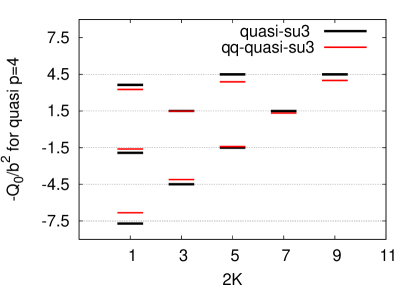
Figure 3: (color online) The Zuker Retamosa Poves (ZRP) diagrams. Top: Intrinsic states in the $p$=4 $gds$ space for the quasi-SU3 model and for the exact $q\cdot q$ calculation. See text for explanation of thin lines. Bottom: Intrinsic states of SU3 or pseudo-SU3 for $p=2$ and 4. For the former exact $q\cdot q$ values (’qq-pseudo’) are also shown. Each orbit may contain two neutrons and two protons. The lowest six orbits are common to $p=2$ and 4.

Table 1: Eigenvalues of $-2q^{20}$ for the i-th quasi–$gds$ (denoted q) and pseudo–$r_{3}$ (denoted p) orbits; q-s, p-s for the results using the schematic quasi and pseudo quadrupole forces in Fig. 3. q-d, p-d are the results of diagonalizing the exact quadrupole interaction; c-q and c-p are the corresponding cumulated absolute values for n particles in units of $b^{2}$

. i 1 2 3 4 5 6 7 8 9 q-s -7.71 -4.50 -1.92 -1.50 1.50 1.50 3.64 4.50 4.50 q-d -6.83 -4.11 -1.61 -1.42 1.33 1.48 3.26 3.90 4.00 p-s -4.00 -1.00 -1.00 2.00 2.00 2.00 p-d -5.06 -1.41 -1.08 2.37 2.57 2.61 $Q_{0}$ values for $n$ particles (c-q for $gds$ and c-p for $r_{3}$) n 4 8 12 16 20 24 28 32 36 c-q 27.32 43.76 50.20 55.88 50.56 44.64 31.60 16.00 0.00 c-p 20.24 25.88 30.20 20.72 10.44 0.00

Table 1 compares the schematic orbits of Fig. 3 with the ones obtained by diagonalizing $2q^{20}$ associated to “true” $2q\cdot 2q$ and not one of its variants. The two bottom lines give the cumulated values after filling up to i-th orbit with 2 neutrons and 2 protons. Thus for 12 particles in $r_{3}$ and 4 in $gds$ we find $\langle 2q^{20}\rangle\,$=30.20+27.32=50.52. This table is the relevant one for prolate states.

Quasi SU3 strongly prefers prolate solutions as Fig. 3 makes clear: it is more advantageous to fill orbits from below than from above.

Table 2: Top: Intrinsic prolate and oblate quadrupole moments $\langle 2q^{20}\rangle\,$for $\nu$ particles in the 0$g_{9/2}$ orbit (N=Z). Bottom: pseudo-SU3 $\langle 2q^{20}\rangle\,$for $\mu$ prolate particles (p-p) or $\mu$ prolate holes (p-h), -$\langle 2q^{20}\rangle\,$for $\mu$ oblate particles (-(o-p)) or $\mu$ oblate holes (-(o-h))

$\nu$	2	4	6	8	10	12	14	16
prol	5.33	10.66	14.66	18.66	20	21.33	18.66	16
-obl	8	16	18.66	21.33	20	18.66	14.66	10.66
$\mu$	2	4	6	8	10	12	14	16
p-p; -(o-h)	10.12	20.24	23.04	25.88	28.05	30.20	25.46	20.72
p-h; -(o-p)	5.22	10.44	15.66	20.72	25.46	30.20	28.04	25.88

III.0.4 Single orbit quadrupole

When the $g$ orbit becomes sufficiently depressed with respect to its $ds$ partners their influence can be neglected and we move to the single $j$ orbit regime with quadrupole moments given by

$$Q_{0}=2\langle r^{2}C_{2}\rangle=\sum_{m}(p+3/2)\frac{j(j+1)-3m^{2}}{2j(j+1)}$$ (6)

which shows that, before midshell, filling large $m$ values (negative $Q_{0}$) is favored. The situation is reversed after midshell. Though the notion of shape is questionable in this case, states with positive and negative $Q_{0}$ will be referred to as prolate and oblate respectively.

Table 2 collects the possible values of $\langle 2q^{20}\rangle\,$for the $g_{9/2}$ orbit and the $r_{3}$ space where one may wish to speak in terms of holes rather than particles, and the table allows for all possibilities. For example, under $\mu$=8 we find that $\langle 2q^{20}\rangle\,$=25.88 for prolate particles, 20.72 for prolate holes, -25.88 for oblate holes and -20.72 for oblate particles.

To guarantee a bona fide intrinsic state, $Q_{0}$ must coincide with the values extracted either from the spectroscopic quadrupole moment ($Q_{0s}$)

$$Q_{spec}(J)=<JJ|3z^{2}-r^{2}|JJ>$$

$$Q_{0s}=\frac{(J+1)\,(2J+3)}{3K^{2}-J(J+1)}\,Q_{spec}(J),\quad K\neq 1$$ (7)

for Bohr Mottelson rotors, or the corresponding B(E2) transitions ($Q_{0t}$)

$$B(E2,J\;\rightarrow\;J-2)=$$

$$\frac{5}{16\pi}\,e^{2}|\langle JK20|J-2,K\rangle|^{2}\,Q_{0t}^{2}\quad K\neq 1/2,\,1$$ (8)

The condition $Q_{0}\approx Q_{0s}\approx Q_{0t}$ is well fulfilled by SU3 states and its variants. ($Q_{0s}$ may be tricky though, as it is more sensitive to details than $Q_{0t}$. For an example refer to section V.1.2 ).

IV Computational Strategy. SU3-Nilsson selfconsistency

The guiding idea is that once quadrupole dominance sets in, the wavefunctions are basically given by the quadrupole force which is quite immune to single particle details. In other words $\langle 2q^{20}\rangle\,$varies little. Our aim is to estimate $\langle 2q^{20}\rangle\,$and understand the reason for its stability.

We shall be interested in even $N=Z=$ 28 to 48 nuclei. Full $pf$ diagonalizations are possible but their interest is restricted to the lightest species. For $r_{3}g$ exact calculations are also possible that account for oblate states. The JUN45 interaction jun45 will be used throughout the region. Though the $r_{3}g$ space is of limited relevance, the exact calculations will serve as a test of our simple models. For the more collective prolate states the full $r_{3}gds$ space is necessary and exact calculations are not presently feasible, so we shall introduce a selfconsistent version of Nilsson’s model that reduces to quasi and pseudo SU3 in the absence of a central field gz .

IV.1 Example of naive $\bm{BE2}$ estimate

For SU3 the correct value of $Q_{0}$ to be used in Eqs. (7, 8) is $Q_{0}=$($\langle 2q^{20}\rangle\,$+3)$b^{2}$ su3 ; scissors with $\langle 2q^{20}\rangle\,$given in Tables 1 or 2. In what follows we adopt this form in all cases.

The procedure is simple: use the tables to match oblate pseudo SU3 states in $r_{3}$ to oblate states in $g$ and prolate pseudo SU3 states in $r_{3}$ to prolate quasi SU3 states in $gds$. For instance: choose 16 particles and decide that we are interested in ⁷²Kr configurations with 12 particles in $r_{3}$ and 4 above. From the tables we have for $\langle 2q^{20}\rangle\,$the following possibilities:

Oblate

$\langle 2q^{20}\rangle\,$= –30.2 for m=12 in pseudo,

$\langle 2q^{20}\rangle\,$= –16 for n=4 in $g$.

Total $Q_{0}/b^{2}$= -(30.2+3+16)= -49.2

Prolate

$\langle 2q^{20}\rangle\,$= 30.2 for m=12 in pseudo,

$\langle 2q^{20}\rangle\,$=27.32 for n=4 in quasi.

Total $Q_{0}/b^{2}=$ 30.2+3+27.32=60.52

Recover dimensions through

$b^{2}\approx 41.4/$$\hbar\omega\,$fm²,   $\hbar\omega\,$=$45A^{-1/3}-25A^{-2/3}$

Now assume a conventional 2$\hbar\omega\,$scalar effective charge, $e_{0}=e_{\nu}+e_{\pi}=2$ chosen throughout in what follows. Then, for $A=72$, $b^{2}=4.42$ $e$fm² , we have $Q_{0}\approx-$217 $e$fm² (oblate); 267 $e$fm² (prolate).

The 2$\hbar\omega\,$effective charge is caused by coupling states in a major HO shell to the giant quadrupole resonance. A rigorous derivation leads $e_{0}$=1.77 mdz , a number to be preferred crawford_eff , and shown in parenthesis below. Using $B(E2:2^{+}\to 0^{+})$ $=[Q_{0}]^{2}/50.3$ from Eq. (8) leads to

$B(E2:2^{+}\to 0^{+})$ $\approx$ 936 (725) e²fm⁴ for oblate;

$B(E2:2^{+}\to 0^{+})$ $\approx$1422 (1101) e²fm⁴ for prolate.

When working in EI or EEI spaces it becomes necessary to account for 0$\hbar\omega\,$polarization effects. In our case due to coupling to the lowest $J=2^{+}$ state in ⁵⁶Ni. The effect will be estimated later leading to $e_{0}\gtrapprox 2$.

IV.2 Nilsson revisited: the MZ equations

The estimates above neglect single particle effects. To account for them demands solving the Schrödinger equation for the quadrupole force in the presence of a central field, a task as hard as the general problem. In reference a4749 Martínez Pinedo and Zuker (MZ) proposed to reduce it, by linearization, to a Nilsson type Hamiltonian. That this should be possible seems obvious but the implementation is not trivial. Because of a subtlety that was missed at the time, the project was left unfinished. We retake it.

We would like to solve

$$H_{mq}=\sum\epsilon_{i}n_{i}-\hbar\omega\kappa\left(\frac{2q_{p}}{{\cal N}_{2q,p}}+\frac{2q_{p+1}}{{\cal N}_{2q,p+1}}\right)^{2}$$ (9)

$${\cal N}_{2q,p}^{2}=\sum(2q_{rs})^{2}=\frac{5}{2}\sum_{k=0}^{p}(k+1)(2p-3k)^{2}$$ (10)

where we have borrowed from mdz the normalized form of the quadrupole force that emerges naturally when it is extracted from a realistic interaction ($q_{p}$ is the quadrupole operator in major shell $p$, the square stands for scalar product). This form ensures that $\kappa\approx 0.22-0.25$ is a universal constant that demands a 30% renormalization due to coupling to the 2$\hbar\omega\,$quadrupole degrees of freedom mdz . It also ensures that nuclei do not become needles, thus solving the crippling problem of the naive quadrupole force bk68 . In all that follows we have fixed $\kappa=0.3$.

To prepare for linearization replace $q$ by $q_{20}$ operators (notice that we use sometimes $q_{20}$ instead of $q^{20}$ for typographical reasons) .

$$H_{mq0}=\sum\varepsilon_{i}n_{i}-\hbar\omega\kappa\left(\frac{2q_{20,p}}{{\cal N}_{2q_{20,p}}}+\frac{2q_{20,p+1}}{{\cal N}_{2q_{20,p+1}}}\right)^{2}$$ (11)

$${\cal N}_{2q_{20,p}}^{2}=\sum(2q_{20,rs})^{2}=\sum_{k=0}^{p}(k+1)(2p-3k)^{2}$$ (12)

Note that Eq. (12) is obtained by summing the squares of the levels in Fig. 2.

Now concentrate on a single space. The operation amounts to replacing $2q\cdot 2q$ by $2q_{20}2q_{20}$, and demands some care because $q_{20}$ is a sum of neutron and proton contributions $q_{20}=q_{20}^{\nu}+q_{20}^{\pi}$. As calculations will be done for each fluid separately, the correct linearization for the neutron operators, say, is:

$q_{20}\,q_{20}\to q_{20}^{\nu}\langle q_{20}^{\nu}+2q_{20}^{\pi}\rangle\approx 3q_{20}^{\nu}\langle q_{20}^{\nu}\rangle$ if $\langle q_{20}^{\nu}\rangle\approx\langle q_{20}^{\pi}\rangle$

leading to the Martínez Zuker (MZ) equation

$$H_{mq0}=\sum\varepsilon_{i}n_{i}-\frac{3\hbar\omega\kappa}{{\cal N}^{2}_{2q_{20},p}}\langle 2q_{20}^{\nu}\rangle 2q_{20}^{\nu}$$ (13)

The subtlety missed in a4749 was the need to change ${\cal N}_{2q,p}$ into ${\cal N}_{2q_{20},p}$ in going from Eq. (9) to Eq. (11), thus making it impossible to discover the proper way to proceed which now can be implemented gz .

To find the proper generalization of Eq. (13) note that in the full space $q$ becomes a sum of four contributions $q_{20}=q_{20}^{\nu u}+q_{20}^{\pi u}+q_{20}^{\nu d}+q_{20}^{\pi d}$ ($u=gds$, $d=r_{3}$). By repeating the arguments leading to Eq. (13) and setting ${\cal N}_{i}={\cal N}_{2q_{20},i}$ leads to the general MZ equation

$$H_{sp}-4\hbar\omega\kappa\frac{q_{4}^{\nu}}{{\cal N}^{2}_{4}}\left(\langle q_{4}^{\nu}\rangle+\langle 2q_{4}^{\pi}\rangle+\langle 2q_{3}^{\nu}\rangle\frac{{\cal N}_{4}}{{\cal N}_{3}}+\langle 2q_{3}^{\pi}\rangle\frac{{\cal N}_{4}}{{\cal N}_{3}}\right)$$

$$\approx H_{sp}-4\hbar\omega\kappa\frac{q_{4}^{\nu}}{{\cal N}^{2}_{4}}\left(3\langle q_{4}^{\nu}\rangle+6\langle q_{3}^{\nu}\rangle\right)$$

$$=H_{sp}-\beta\hbar\omega\kappa\frac{\langle 2q_{4}^{\nu}\rangle}{{\cal N}^{2}_{4}}2q_{4}^{\nu}$$ (14)

where we have introduced a boost factor $\beta$, set $q_{i}^{\nu}=q_{i}^{\pi}$ and used the correct numbers from Eq. (12) ${\cal N}_{2q,3}=\sqrt{90\times 2.5}\approx 15$, ${\cal N}_{2q,4}=\sqrt{210\times 2.5}\approx 23$. to approximate ${\cal N}_{4}/{\cal N}_{3}=22.91/15\approx 1.5,$

As the $\langle 2q^{20}\rangle\,$ranges will be $\langle 2q_{3}\rangle\approx 30$ and $\langle 2q_{4}\rangle=27-55$, the modest value of $\beta=3$ in Eq. (13) will increase to about $\beta=9$-12, but the work involved in solving Eqs. (13) and (14) is identical.

Let us examine the steps involved.

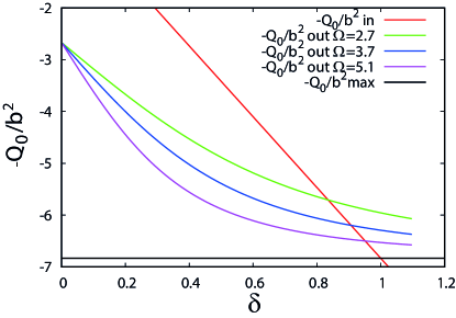
Figure 4: (color online) Calculation of $\langle 2q_{20}\rangle$ in $(gds)^{4}$. Input values in red. Output values obtained solving Eq. (13) for $\varepsilon_{i}=0$,1,2 MeV for $i=g,d,s$ respectively. When input and output values coincide, selfconsistency is achieved i.e., when lines cross, which happens at abscissae 0.83, 0.91, 0.95 for $\Omega=\hbar\omega\kappa=$ 2.7, 3.7, 5.1 respectively. At $\delta=0$ $\langle 2q^{20}\rangle\,$=2.666 corresponds to one prolate $g$ orbit (from Table 2)

a) Eq. (13) is solved setting as inputs $\langle 2q_{20in}\rangle=\delta\langle 2q_{20max}\rangle$, which for $\delta=1$ yields the maximum value of $\langle 2q_{20}\rangle$ (the one obtained at $\varepsilon_{i}=0$). The resulting eigenvalue can be written as

$$E(\delta)=\langle H_{sp}\rangle-\frac{3\hbar\omega\kappa}{{\cal N}^{2}_{2q_{20}}}\delta\langle 2q_{20max}\rangle\langle 2q_{20out}\rangle$$ (15)

b) Extract $\langle 2q_{20out}\rangle$, use it as next input and iterate until $\langle 2q_{20in}\rangle=\langle 2q_{20out}\rangle$. Fig. 4 sums up the procedure.

c) Guess energies. The comparison of the resulting $\langle 2q_{20out}\rangle=Q_{0}/b^{2}$ with exact results turns out to be systematically satisfactory. Some examples are given in Section IV.3. As a reasonable estimate of $Q_{0}/b^{2}$ amounts to a good guess of intrinsic state from which the energy could be extracted by taking the expectation value of $H_{mq}$ in Eq. (9) but it is more instructive and simpler to stand by our basic assumption that $2q_{20}$ is an acceptable quantum number and rely on the exact SU3 result as a guide.

$$E=-\frac{\hbar\omega\kappa}{{\cal N}_{2q}^{2}}\left(2\lambda(2\lambda+6)+2\mu(2\mu+6)+4\lambda\mu-3L(L+1)\right)$$

where $\lambda$ and $\mu$ are the difference in quanta in the z and x, and x and y directions respectively. This result is valid for the $q\cdot q$ force that contains one and two body parts. As we are not interested in the former we expect modifications if they are neglected. Moreover, we shall restrict the energy estimates to $(\lambda 0)$ representations because the only obviously correct identification in the absence of external monopole fields is 2$\lambda=$$\langle 2q^{20}\rangle\,$. The idea is to assume that the quadrupole contribution to the energy keeps this form using the calculated $\langle 2q^{20}\rangle\,$value.

The proposed estimates are as follows

$$BE2=B(E2:2^{+}\to 0^{+})=((\langle 2q_{20}\rangle+3)b^{2})^{2}/50.3$$

$$Q_{s}=Q_{(J=2)s}=(\langle 2q_{20}\rangle+3)b^{2}/3.5$$

$$E=\langle H_{sp}\rangle-\frac{\hbar\omega\kappa}{{\cal N}_{2q}^{2}}\langle 2q_{20}\rangle(\langle 2q_{20}\rangle+\zeta)$$ (16)

For $Q_{s}$ and $B(E2:2^{+}\to 0^{+})$ we use Eqs. (7-8). The norms are those of the full quadrupole interaction i.e., ${\cal N}_{2q}=\sqrt{2.5}{\cal N}_{2q20}$. The parameter $\zeta$ in the form of $E$ should be 6 if the SU3 analogy held perfectly. However, as hinted above and made evident in next section IV.3 this is not possible and $\zeta$ must be viewed as an artifact to estimate uncertainties in the guessed energies.

Finally, let us propose a generalization of Eq (16) for the the energy of a $r_{3}^{k}(gds)^{l}$ configuration, and write explicitly $Q_{s}$ and $B(E2:2^{+}\to 0^{+})$ Calling $\langle 2q_{20(i)}\rangle=Q_{i}$, we have

$$BE2=B(E2:2^{+}\to 0^{+})=((Q_{3}+Q_{4}+3)b^{2})^{2}/50.3$$

$$Q_{s}=Q_{(J=2)s}=(Q_{3}+Q_{4}+3)b^{2}/3.5$$

$$E=H_{m}-\hbar\omega\kappa(\frac{Q_{3}}{15}+\frac{Q_{4}}{23})(\frac{Q_{3}+\zeta}{15}+\frac{Q_{4}+\zeta}{23})$$ (17)

where the monopole term $H_{m}$ subsumes the evolving behavior of the single particle fields to be discussed in Section V.2.

IV.3 Pseudo and Quasi SU3 as exact symmetries

According to SU3, ²⁸Si has a prolate-oblate degenerate ground state corresponding to the $(\lambda,\,\mu)=$ (12,0) and (0,12) representations. This holds for the full $q\cdot q$, i.e., including both its one and two body terms. If the former are ignored we obtain the results in the right upper panel of Table 3, which show no signs of an exact degeneracy. The estimated energy using $\zeta=0$ in Eq. (16) is about 5% larger than the exact one. Nearly perfect degeneracy is achieved with the monopole free $q\cdot q$—i.e., with all centroid averages set to 0—in the left upper pannel and the estimated energy with $\zeta=3$ is now some 5% too small.

Table 3: $q\cdot q$ calculations in ²⁸Si($(sd)^{12}$) (upper panels) and ⁶⁸Se($r^{12}_{3}$) (lower panels). To the left $q\cdot q$ is made monopole free. “Int” stands for intrisic values defined in Eq. (16), with $\zeta=3$ in the left panel and 0 in the right one. Absolute energies given for the ground state, excitation energies for the other states (MeV).

J	$E$	$Q_{s}$	$BE2$	J	$E$	$Q_{s}$	$BE2$
0	-27.26329			0	-22.044
0	0.00192			2	0.958	-26.330	166.979
2	0.91714	-0.7785	167.299	0	1.646
2	0.91730	0.7785	167.301	2	2.494	26.323	166.903
Int	-26.20	-26.40	169.74	Int	-23.23	-26.40	169.74
0	-14.97822			0	-12.176
0	0.00042			2	0.533	-42.087	426.802
2	0.50677	-2.8707	427.591	0	0.996
2	0.50683	2.8708	427.590	2	1.467	42.117	426.915
Int	-13.99	41.21	413.64	Int	-12.73	41.21	413.64

The story repeats itself in the lower panels for ⁶⁸Se: a remarkable result establishing that pseudo-SU3 behaves as an exact symmetry in this case. A puzzling result since we are using the true $q\cdot q$ potential whose matrix elements coincide in magnitude with their pseudo counterparts but have different sign structure. So much so that their overlaps (in the sense of (rmp, , Eq.(44))) nearly vanish.

Let us draw some conclusions.

• Energies are very sensitive to monopole behavior but $B(E2:2^{+}\to 0^{+})$ rates are not.

• When bands—with equal $B(E2:2^{+}\to 0^{+})$ and opposite $Q_{s}$—cross, they mix leading to unchanged $B(E2:2^{+}\to 0^{+})$ and cancellation of $Q_{s}$. Note that this could happen through small “impurities” in the Hamiltonian. If the symmetry were exact, the Lanczos algorithm used in the diagonalizations could not break the degeneracy.

• Pseudo SU3 appears to be close to an exact symmetry.

IV.4 Checks

Allowing the single particle energies to vary produces more stringent tests of the estimates in Eq. (16). Numerous calculations done for the $r_{3}^{n}$ and$(gds)^{n}$ spaces lead to results that are well summarized by the examples in Table 4.

Table 4: Monopole-free $q\cdot q$ calculations in $(gds)^{8-12}$. Single particle energies in MeV: $\varepsilon_{i}$=[0.0, 0.0 and 0.0](e0) and [0.0, 1.0, and 2.0](e1) for $i=g,\,d,\,s$ respectively. “Int” stands for intrisic values defined in Eq. (16) with $\zeta=3$.

J	$E$	$Q_{s}$	$BE2$	J	$E$	$Q_{s}$	$BE2$
$(gds)^{8}$ e0				$(gds)^{8}$ e1
0	-12.977			0	-8.976
2	0.113	-59.735	857.959	2	0.103	-57.313	795.566
Int	-12.34	-59.98	876.05	Int	-8.28	-57.50	805.07
$(gds)^{12}$ e0				$(gds)^{12}$ e1
0	-17.894			0	-12.641
2	0.125	-65.296	1161.574	2	0.136	-65.609	1065.721
Int	-15.84	-69.16	1165.04	Int	-8.63	-67.49	1109.34

In all cases the selfconsistent calculations do well for the quadrupole properties. The estimated energies in $(gds)^{8}$ are also satisfactory, but they fall short for $(gds)^{12}$ which is triaxial because the platform at $\langle 2q^{20}\rangle\,$=-1.5 in Fig. 3 is not fully filled, leading to $\mu\neq 0$ while $E$ in Eq. (16) is designed for $\mu=0$ only.

V N=Z nuclei

Granted the benefit of some hindsight, a reading of Fig. 3 suggests three regimes for $N=Z$ nuclei from ⁵⁶Ni up to ⁹⁶Cd. Note that placing the $gds$ “quasi” orbits on top of the “pseudo” $r_{3}$ ones was designed to facilitate such a reading.

i) The $r_{3}$ pseudo SU3 nuclei. They fill orderly the three lowest levels in Fig. 3: ⁶⁰Zn (analog of ²⁰Ne in the $sd$ shell, a mild rotor), ⁶⁴Ge (analog of ²⁴Mg, a rotor exhibiting a $\gamma$ band, as expected whenever orbits are not all filled at a given level), ⁶⁸Se (analog of ²⁸Si, with degenerate prolate and oblate bands). While SU3 dominance is largely frustrated in the $sd$ shell, here it is expected to hold well because of the near degeneracy of the single particle orbits. This region makes it possible to study the full $pf$ to $r_{3}$ reduction: A unique opportunity to validate the notion of model space and in particular the assumption that ⁵⁶Ni can be treated as a closed shell. As for $r_{3}g$ calculations kaneko , they add little to the $r_{3}$ ones.

ii) Coexistence from ⁷²Kr to ⁸⁴Mo. For 12 particles, i.e., ⁶⁸Se, $\langle 2q^{20}\rangle\,$reaches a maximun in $r_{3}$ (see last lines of tables 1 and  2). Adding particles to the pseudo orbits leads to a loss while adding them to the quasi orbits leads to a gain. By filling the quasi orbits, well deformed prolate states can be constructed for 4, 8, 12 and 16 particles whose quadrupole energy will overcompensate the monopole (i.e., single particle) losses. Oblate states very close in energy can also be found, leading to coexisting bands. The prolate and oblate states demand $r_{3}gds$ and $r_{3}g$ spaces respectively. The associated dimensionalities exceed $10^{14}$ for the former and $10^{10}$ for the latter—still large but feasible. Therefore we shall rely on a generalization of the simplified approach of Section IV.3 for both deformations and check the oblate results via exact diagonalizations. For studies of the region see vampir ; 64-84 .

iii) The $r_{3}g$ nuclei ⁸⁸Ru ⁹²Pd and ⁹⁶Cd. The second has been measured recently ceder:10 and postulated as candidate for a new form of boson aligned collectivity. We shall examine the claim. The—still unknown—spectrum of ⁹⁶Cd will be shown to be probably closer to $sdg$ than to $r_{3}g$.

V.1 The $\bm{pf}$ to $\bm{r_{3}}$ reduction

Doubts may be raised about the doubly magic nature of ⁵⁶Ni as its first 2⁺ is rather low and, depending on the effective interaction used (kb3g, gxpf1a) kb3g ; gxpf1a the closed shell component amounts to only 60-70%. However, it is in the nature of the shell model to recognize that there may be a difference between the potentially complicated structure of a state and its simple behavior. As a first hint of what is expected of magic nuclei we refer to Figures 1–5 in alpha : at magic numbers, two-neutron and two-proton separation energies exhibit systematic jumps. Clearly the case for $N$ or $Z=\,$28, and a fortiori for ⁵⁶Ni. Not for occasional candidates such as $N=56$ which is magic only for $Z=40$.

For our present purpose the state of interest is the head of the 4p-4h rotational band. According to Eq. (6) four holes in the 0f_7/2 orbit give a prolate contribution of 12b² to the intrinsic quadrupole moment while four pseudo SU3 particles in $r_{3}$ contribute with $\approx$ 22b², adding up to 34b² in agreement with 32b² from a full 4p-4h $pf$-shell calculation. A first example of the use of our schematic coupling schemes.

V.1.1 0$\hbar\omega\,$polarization

The most important characteristic of a doubly magic nucleus is that it defines a before and an after. Before ⁵⁶Ni, nuclei are basically of $f$ type. Beyond, they are at first of $r_{3}$ type until the extension to $r_{3}gds$ spaces becomes imperative. To treat ⁵⁶Ni as a core, the Hamiltonian and transition operators have to be renormalized. The dominant mechanism involves coupling to the low lying $2^{+}$ state, leading to three-body forces and two-body effective transition operators Pb (i.e., state dependent effective charges) whose neglect, as stressed in ref. mdz , is “common but bad practice”. Short of a rigorous treatment we chose the following expediencies:

• For the energies we assume that jun45 jun45 provides a reasonable approximation to the effective Hamiltonian. To fix ideas: in mdz it is shown that for the quadruplole component of the bare realistic forces the 2$\hbar\omega\,$effects demand a 30% boost (consistent with what is known about phenomenological interactions). As a consequence the effective $q\cdot q$ amounts to about 50% of the total interaction. In the case of jun45 it jumps to over 75%, indicating a strong contribution due to 0$\hbar\omega\,$mechanisms.

• For the transition operators we proceed by brute force, estimating effective charges by comparing full $pf$ transitions rates to those obtained in the $r_{3}$ or $r_{3}g$ spaces.

V.1.2 ⁶⁰Zn, more on magicity

To check that ⁶⁰Zn is properly described by $r_{3}^{4}$ configurations we do a full $pf$ diagonalizations which involves 2.292.604.744 M=0 Slater determinants. The story is told in Table 5. A calculation in the $r_{3}$ space, using a pure quadrupole-quadrupole interaction gives values in the range 24b². As expected we have good rotational features including $J(J+1)$ spacings. The full $pf$-shell calculation using the kb3gr interaction kb3gr accounts well for the experimental spectrum. The $J(J+1)$ spacings are gone but this is of little consequence. As abundantly emphasized in  zrpc what matters is the wavefunction i.e., the quadrupole moments. The spectrum may be sensitive to details detected in first order perturbation theory that do not change the structure of the state. And the message from Table 5 is that the quadrupole moments of the huge calculation and the modest one are compatible, to within a crucial caveat: The full $pf$ space leads to $Q_{0t}$ values that are about 1.36 times bigger than the $r_{3}$ ones. As the coupling is mediated basically by the $p_{3/2}f_{7/2}^{-1}$ jumps the renormalization decreases as the $p_{3/2}$ orbit gets filled thus blocking the jumps. The results hardly change when jun45 is used instead of $q\cdot q$ in the $Q_{0t,qq}$ column of Table 5, 23 goes to 20.8, increasing the enhancement factor $F$ from 1.36 to 1.48. The calculated spectrum—though still dilated—comes closer to the experimental one.

Note that the evolution of $Q_{0s}$ and $Q_{0t}$ are quite different. In general the two quantities will be approximately equal only in the case of well developed rotors. More often than not $Q_{s}$ is very sensitive to details, while $Q_{t}$ is close to the predictions from Tables 1 and 2.

Table 5: Properties of the yrast band of ⁶⁰Zn ($E$ in MeV, $Q$ in units of b²).Calculations: full $pf$ with kb3gr; and $r_{3}$ with $q\cdot q$.

J	$E_{exp}$	$E_{qq}$	$E_{pf}$	$Q_{0s,qq}$	$Q_{0s,pf}$	$Q_{0t,qq}$	$Q_{0t.pf}$
2+	1.00	1.00	1.07	24	22	23	31
4+	2.19	3.34	2.31	23	25	22	30
6+	3.81	7.03	4.06	23	14	19	31

It is worth mentioning that ⁶⁰Zn has a superdeformed excited band at relatively low energy with $Q_{0}$= 67(6) b² sd60zn . From Tables II and III two prolate candidates emerge with configurations $f^{12}r_{3}^{4}(gds)^{4}$ and $f^{12}(gds)^{8}$. Both are consistent with observation.

V.1.3 ⁶⁴Ge

Table 6: Properties of low lying states in ⁶⁴Ge, Energies in MeV, $B(E2)$ in $e^{2}$fm⁴ . Calculations: full $pf$ with gxpf1a ge64 ; $r_{3}g$ with jun45 and $r_{3}$ with $q\cdot q$.

$J^{\pi}$		Exp	$pf$	$r_{3}g$	$q\cdot q$
2${}^{+}_{1}$	$E_{x}$	0.90	0.94	0.86	0.50
2${}^{+}_{1}$	$Q_{s}$		-18.6	-24.4	5.03
	$B(E2:2_{1}^{+}\rightarrow 0_{1}^{+})$	410(60)	406	251	300
2${}^{+}_{2}$	$E_{x}$	1.579	1.56	1.27	0.55
2${}^{+}_{2}$	$Q_{s}$		18.5	23.3	-5.42
	$B(E2:2_{2}^{+}\rightarrow 2_{1}^{+})$	620(210)	610	182	479
	$B(E2:2_{2}^{+}\rightarrow 0_{1}^{+})$	1.5(5)	14	13	39
4${}^{+}_{1}$	$E_{x}$	2.053	2.00	2.16	1.61
	$B(E2:4_{1}^{+}\rightarrow 2_{1}^{+})$		674	314	390

For ⁶⁴Ge the diagonalization of the $q\cdot q$ interaction in the $(r_{3})^{8}$ space yields the expected results for an (84) SU3 representation with nearly degenerate 2⁺ states—with $Q_{0}$ of equal magnitude and opposite signs—corresponding to the $K$=0 and 2 ground state and $\gamma$ bands respectively, and $B(E2:2^{+}\to 0^{+})$ of about 300 $e^{2}$fm⁴ . Table 6 proposes a comparison of $q\cdot q$ and jun45 results—in $r_{3}$ and $r_{3}g$ spaces respectively—with data, well reproduced by gxpf1a calculations ge64 . Using as reference the $B(E2:2^{+}\to 0^{+})$ values it is found that in going from $r_{3}$ to $pf$ the enhancement factors $F$ are 1.62 (for jun45) and 1.23 (for $q\cdot q$).

V.1.4 ⁶⁸Se: The double platform

The structure of $N=Z$ even nuclei from $A=$72 to 84 will be described by piling up $(gds)^{4}$ blocks on top $r_{3}^{12}$, i.e., on top of either the oblate and prolate ground state bands—corresponding to the (12 0) and (0 12) SU3 representations—of ⁶⁸Se which becomes a common “double platform” (refer to Fig. 3). Hence the importance of this nucleus to fix the $e_{0}$ effective charge.

Table 7: Properties of low lying states in ⁶⁸Se, Energies in MeV, $B(E2)$ in $e^{2}$fm⁴ . Calculations: full $pf$ with gxpf1a ge64 ; $r_{3}$ with jun45: $r_{3}$ with $q\cdot q$; and full $pf$ with kb3gr ($PF$). The experimental $0^{+}_{2}$ energy is a guess.

$J^{\pi}$		Exp	$pf$	$r_{3}$	$q\cdot q$	$PF$
0${}^{+}_{2}$	$E_{x}$	(1.19)	0.69	0.96	0.79	1.42
2${}^{+}_{1}$	$E_{x}$	0.85	0.71	0.54	0.53	0.96
2${}^{+}_{1}$	$Q_{s}$		11	35	-42	39
	$B(E2:2_{1}^{+}\rightarrow 0_{1}^{+})$	440(60)	491	307	420	409
2${}^{+}_{2}$	$E_{x}$	1.59	1.00	1.39	1.26	1.74
2${}^{+}_{2}$	$Q_{s}$		-8	-33	42	-16
	$B(E2:2_{2}^{+}\rightarrow 2_{1}^{+})$		689	7	0.00	297
	$B(E2:2_{2}^{+}\rightarrow 0_{2}^{+})$		499	262	420	223
	$B(E2:2_{2}^{+}\rightarrow 0_{1}^{+})$	0.3	4	0.7	0.00	10
4${}^{+}_{1}$	$E_{x}$	1.94	1.66	1.61	1.77	1.86
4${}^{+}_{1}$	$Q_{s}$		59	43	-53	63
	$B(E2:4_{1}^{+}\rightarrow 2_{1}^{+})$		590	419	565	810
4${}^{+}_{2}$	$E_{x}$	2.55	1.98	2.28	2.37	2.79
4${}^{+}_{2}$	$Q_{s}$		-51	-42	53	-14
	$B(E2:4_{2}^{+}\rightarrow 2_{2}^{+})$		510	354	565	154

From Table 1 the estimate $Q_{0}/b^{2}=\pm 33.2$ i.e., $B(E2:2^{+}\to 0^{+})$ $\approx 414$ $e^{2}$fm⁴ , consistent the $q\cdot q$ numbers in Table 7, which also collects jun45 results in $r_{3}$, the full $pf$ gxpf1a and kb3gr ones (labeled $pf$ and $PF$ respectively) and data including the only experimentally known $B(E2:2^{+}\to 0^{+})$ = 440(60) e²fm⁴.

With the exception of the $B(E2:2_{2}^{+}\rightarrow 2_{1}^{+})$ the calculations in $r_{3}$ and $pf$ are quite consistent, with enhacement factors $F\approx$ 1.16 and 1.38 for the $q\cdot q$ and jun45 numbers respectively. The kb3gr interaction yields somewhat better spectra than gxpf1a, and similar quadrupole properties except for the $J=2^{+}_{2}$ and $4^{+}_{2}$ states that are more mixed for the latter.

Using the 2$\hbar\omega\,$value $e_{0}=$1.77 mdz , the 0$\hbar\omega\,$contribution increases it to $e_{0}=1.77\sqrt{F}\approx 2.1\pm 0.1$. When $gds$ particles come into play their quadrupole operators will also couple with the $J=2^{+}$ state in ⁵⁶Ni, though more weakly due to larger norm denominators (see Eqs. (9 and 17)). It is hoped that the associated suppression can be accommodated by the proposed estimate.

The jun45 calculation in $r3g$ leads to a ground state that is 60% 0p-0h, 30% 2p-2h and 10% 4p-4h. As can be gathered from Tables I and II these admixtures bring no extra oblate coherence but with the same numbers, prolate contributions could make a difference in a full $r_{3}gds$ calculation. Vampir calculations vampirse indicate substantial oblate-prolate mixing in the ground state band. Further data on this nucleus could be of interest.

V.2 The central region: A=72 to 84

Let us recast $E$ in Eq. (17) so as to separate the two basic contributions to the monopole term $H_{m}$.

$$E=\sum\varepsilon_{i=g,d,s}\langle n_{i}\rangle+l(\varepsilon_{g}-\varepsilon_{r_{3}})$$

$$-\hbar\omega\kappa\left(\frac{Q_{3}}{15}+\frac{Q_{4}}{23}\right)\left(\frac{Q_{3}+\zeta}{15}+\frac{Q_{4}+\zeta}{23}\right)$$

$$=hsp+l\epsilon_{gr}+E_{q}$$ (18)

where we have introduced the notations used in Table 8—the core of this study— which lists the properties of the dominant and subdominant prolate and oblate states.

Table 8: Properties of $r_{3}^{k}(gds)^{l}$ configurations. Total ($E$), quadrupole ($E_{q}$) and single particle ($hsp$) energies from Eq. (18) with $\zeta=0$, in MeV; quadrupole moment $Q_{4}=\langle 2q_{20(4)}\rangle$; $BE2=$$B(E2:2^{+}\to 0^{+})$ in $e^{2}$fm⁴ from Eq. (17); $\beta=8$ in Eq. (14). For prolate states $Q_{4}$ is the calculated one. For oblate states the space is $r_{3}^{k}(g)^{l}$ so $\epsilon_{r_{3}}=0.0$ and $Q_{4}$ (not shown) is from Table 2. $Q_{3}$ is always from Table 2. Energies of triaxial states in boldface. Single particle energies in MeV: $\varepsilon_{i}$=0.0, 3.0 and 4.0 [0.0, 4.0, and 5.0] for $i=g,\,d,\,s$ respectively, and $\epsilon_{gr}=2.5$ [2.0]. Numbers in square brackets apply to the last two lines only.

k	l	A	$E$	-$E_{q}$	$hsp$	$Q_{3}$	$Q_{4}$	$BE2$
12	4	72	-12.29	25.53	3.24	30.20	23.00	1225
16	0	72	-8.37	8.37	0.0			324
12	4	72	-10.63	20.63	0.0			939
12	8	76	-12.29	40.05	7.76	30.20	41.17	2212
16	4	76	-2.46	15.62	3.15	20.72	22.85	867
14	6	76	-4.90	19.90	0.0			987
16	4	76	-6.23	16.23	0.0			805
12	12	80	-0.30	47.01	16.71	30.20	49.15	2792
16	8	80	1.76	27.45	7.69	20.72	41.17	1733
18	6	80	-0.04	15.04	0.0			823
12	16	84	5.91	51.92	17.82	30.20	54.71	3271
16	12	84	13.47	33.20	16.67	20.72	49.01	2240
20	8	84	6.05	13.95	0.0			840
12	16	84	3.02	51.25	22.26	30.20	54.05	3223
20	8	84	2.05	13.95	0.0			840

To ascertain the stability of the estimates, all the calculations, done with $\zeta=0$, have been redone for $\zeta=3$. The examples that follow are for $A=84$ which involves the largest magnitudes for $hsp,\,l\epsilon_{gr}$ and $E_{q}$ and hence, presumably, the largest uncertainties.

For $\zeta=0\to 3$ the energies $E=$5.91, 13.47 and 6.05 in Table 8 go to 4.03, 11.89 and 5.0 respectively, leaving unchanged the qualitative conclusions that may be drawn.

The evolution of the monopole is another source of uncertainty: The $\varepsilon_{i}$ and $\varepsilon_{gr}$ numbers are suggested by GEMO gemo at the beginning of the region. As the $g$ filling increases, the orbit will separate from its $ds$ partners and come closer to the $r_{3}$ space. To simulate this effect, in the last two lines of Table 8 the single particle energies are changed to the bracketed values in the caption. As a consequence the energies at $E=5.91$ and 6.05 change to 3.02 and 2.05 respectively. Again the qualitative conclusions are not affected.

These results for ⁸⁴Mo are typical and illustrate two important points:

1. For prolate states $B(E2:2^{+}\to 0^{+})$ and $\langle 2q^{20}\rangle\,$are very unsensitive to monopole behavior and hence remain close to their theoretical quasi+pseudo SU3 maxima. In our example $Q_{4}$=54.71 and 54.05 against the 55.88 maximum.

2. Energies of prolate states are very sensitive to the single particle field $H_{sp}$. In our example a shift of some 4.5 MeV: $hsp=17.82\,vs$ 22.26 MeV. However, the relative positions of the states remain fairly stable.

Examine now what conclusions can be drawn from Table 8.

⁷²Kr The only species where $B(E2:2^{+}\to 0^{+})$ are close for prolate and oblate candidates. Probable coexistence.

⁷⁶Sr Single candidate. Coexistence ruled out. Experimentally superb rotor with good $J(J+1)$ sequence. Perfect agreement of Table 8 with a recent measure: $B(E2,2^{+}$$\rightarrow$0⁺)= 2220(270) e²fm⁴ be2sr76 .

⁸⁰Zr The lowest state is expected to gain some 4 MeV because of triaxiality and the observed rotational spectrum seems to guarantee $B(E2:2^{+}\to 0^{+})$ close to the prediction. However the very low lying oblate state may blur the picture. Moreover the prolate 8p-8h (and a 10p-10h not shown) are also close and triaxial. Finally, the frustrated doubly magic $N=Z=40$ is at…0. MeV. A very interesting nucleus.

⁸⁴Mo Strong hint of coexistence, even triple coexistence through gains due to triaxiality of the second prolate candidate.

Except for ⁷⁶Sr, coexistence is expected in the other nuclei and will be examined in Section VI.

V.3 The $\bm{r3g}$ calculations

Calculations in the $(r_{3}g)^{n}$ spaces have been carried out for all $n$. We concentrate on results for $A\geq 80$. In particular ⁸⁰Zr and ⁸⁴Mo are mainly of interest in lending support to a basic observation about oblate bands:

Contrary to prolate states that privilege maximizing the deformation, the oblate bands give precedence to mixing that reduces it. As a consequence our schematic estimates overestimate $\langle 2q^{20}\rangle\,$and $B(E2:2^{+}\to 0^{+})$ and underestimate energies.

⁸⁰Zr and ⁸⁴Mo

Table 9: ⁸⁰Zr. Results of the full (1.1$10^{10}$ dimensional) $r_{3}g$ calculation with jun45 (E’s in MeV, $Q$ in efm² and $B(E2:2^{+}\to 0^{+})$ in e²fm⁴)

J	E(2+)	$Q_{s}$	$Q_{0s}$	B(E2)	$Q_{0t}^{2}$
2	0.393	51	-179	642	$(180)^{2}$

In Table 9 the extracted $Q_{0}\approx 180$ is definitely lower than the 6p-6h number from Table 2, $Q_{0}\approx(19+23+3)b^{2}\approx$ 203 $e$fm² . The wavefunctions have 22% 4p-4h, 44% 6p-6h and 28% 8p-8h. Mixing with prolate states nearby may be at the origin of the reduction, as confirmed in Table 10 for ⁸⁴Mo.

Table 10: ⁸⁴Mo. Properties of the yrast band; experiment vs. calculations in the $r_{3}g$ space with the jun45 interaction: to the left truncated up to 4 holes in $r_{3}$. To the right complete space. (E in MeV, $Q$ in $e$fm² and $B(E2)$ in $e^{2}$fm⁴ 

J	Ex	Et	$-Q_{0s}$	B(E2)	$-Q_{0t}$	Et	$-Q_{0s}$	B(E2)	$-Q_{0t}$
0	0.0	0.0				0.00
2	0.44	0.17	194	762	196	0.29	189	708	188
4	1.12	0.56	190	1081	195	0.84	189	1020	189
6	2.01	1.15	184	1179	194	1.60	189	1118	189

The ground state band is dominated now by the $r_{3}^{-4}g^{8}$ configuration. From Table 2 $Q_{0}\approx(21+20+3)b^{2}=44\times 4.61\approx 203$ $e$fm² not inconsistent with the truncated calculations (left of the Table) that exhibit good rotational features. Once the full space is incorporated (right of the Table), the energies depart from the $J(J+1)$ sequence while the quadrupole properties, still those of a rotor, have suffered an erosion due to the inclusion of prolate states as suggested in ⁸⁰Zr.

⁸⁸Ru

Table 11: Properties of the yrast band of ⁸⁸Ru; experiment vs calculations in the $r_{3}g$ space with the jun45 interaction (E in MeV, $Q$ in efm² and $B(E2)$ in e²fm⁴)

. J E(exp) E(th) -Q_s $B(E2\downarrow)$(th) 0${}^{+}_{1}$ 0.0 0.0 2${}^{+}_{1}$ 0.62 0.56 37 492 4${}^{+}_{1}$ 1.42 1.31 44 766 6${}^{+}_{1}$ 2.38 2.12 47 888 8${}^{+}_{1}$ 3.48 2.88 52 980

In ⁸⁸Ru we come at last to a genuine $r_{3}g$ nucleus. (Note that for $A\geq 88$ most numerical results reported below duplicate those of the Rutgers group zamickRuPd ). Table 11 corresponds to an yrast oblate band exhibiting 50% $r_{3}^{-4}g^{12}$ oblate dominance. Not obvious, since $g^{12}$ is now beyond midshell and the largest $\langle 2q^{20}\rangle\,$is prolate. However the oblate $\langle 2q^{20}\rangle\,$in $r_{3}^{-4}$ is sufficiently strong to dominate but the prolate admixtures distort and reduce the original $\langle 2q^{20}\rangle\,$=-(18.66+20.24) and $Q_{0}\approx-182$ to $Q_{0s}\approx-125$ and $Q_{0t}\approx-160$ in Table 11. It is seen that in this nucleus the prolate-oblate competition within the $r_{3}g$ space is played up. ⁹²Pd will bring further news.

⁹²Pd

The authors’ interest in heavy N=Z nuclei was sparked by the first measurement of the ⁹²Pd spectrum, accompanied by an interpretation that associated it to a condensate of $(g_{9/2}^{2})$ neutron-proton pairs coupled to maximum $J=9$ ceder:10 ; chong:11 ; vanI . Which raised two issues: that of possible coupling schemes in a $g^{12}$ space, and that of possible dominance of this configuration. Table 12—which we comment column by column—sums up sufficient information to resolve both issues:

Table 12: Properties of ⁹²Pd. Energies in MeV, $Q$ in efm² and $B(E2)$ in e²fm⁴. Detailed explanation in text

1	2	3	4	5	6	7	8	9	10
J	Ex	Et	con	$qq$	$\Omega$	$B(E2)$	$B(E2)_{r_{3}g}$	$Q_{s}$	$Q_{s,r_{3}g}$
0	0.0	0.0	.00	.00	.99	—	—	—	—
2	0.874	0.84	.26	.22	.99	225	304	-28	-3.63
4	1.786	1.72	.58	.62	.99	316	382	-34	-8.20
6	2.563	2.52	.85	1.20	.98	340	364	-31	-2.77

1. J value

2. Experimental spectrum, in very good agreement with

3. jun45 spectrum.

4. Spectrum of the condensate defined by $-H_{\rm con}$ = P₀ +9P₉, where P₀ and P₉ are the pairing Hamiltonians for $J=0$ and 9.

5. Spectrum of the quadrupole force scaled so as to have unit $J=9$ matrix element. Close to that of the condensate (within arbitrary scaling factor)

6. Overlap, $\Omega=\langle qq|{\rm con}\rangle^{2}$, of the wavefuntions indicating that the condensate and quadrupole coupling schemes are identical. The use of P₉ should be understood as an artifact to define a coupling scheme. As a Hamiltonian it is better avoided.

7, 8. Now for the second issue. A Hamiltonian $-H\approx.6qq+.4P_{0}$ yields $g^{12}$ energies that are close to the exact ones and $B(E2)$ that are very close to the pure $qq$ values in column 7, and not too far from the exact ones in column 8. Which may encourage the idea of $g^{12}$ dominance in spite of its smallish 30% contribution to the exact wavefunction. However, this idea is not supported by the disparity of $Q_{s}$ in columns 9 and 10.

9, 10 Spectroscopic $Q_{s}$ for $qq$ (9) and jun45 jun45 (10).

The situation is reminiscent of that of $f_{7/2}^{n}$ configurations that yield apparently reasonable energetics and transition rates but quadrupole moments of the wrong sign pozu:81 .

The pattern we started following at ⁸⁰Zr—of oblate states progressively eroded by prolate mixtures—now reaches its climax with the Pyrrhic victory of prolate states practically cancelled by oblate mixtures.

⁹⁶Cd

For this nucleus, the calculations in the $r_{3}g$ and $g$ spaces with jun45 give results that are much closer than in ⁹²Pd, both for the energies and for the $B(E2)$ properties and the discrepancies in the spectroscopic quadrupole moments are gone except for the $6^{+}$ state.

Table 13: ⁹⁶Cd. Energies in MeV, $Q$ in $e$fm² and $B(E2)$ in $e^{2}$fm⁴ e²fm⁴

		$\Delta E$			$B(E2)$			$Q_{s}$
$J^{\pi}$	$r_{3}g$	$g_{9/2}$	$sdg$	$r_{3}g$	$g_{9/2}$	$sdg$	$r_{3}g$	$g_{9/2}$	$sdg$
0+	0.0	0.0	0.0
2+	0.90	0.96	0.77	152	154	327	-19	-23	-37
4+	1.91	2.10	1.78	203	206	426	-22	-22	-40
6+	3.02	3.08	2.78	191	159	351	-11	-5	-23
8+	3.48	3.08	3.24	47	40	65	40	39	55

We have collected some results in Table 13, adding those from the full $sdg$ space using the Nowacki-Sieja interaction nara:11 which describes the superallowed decay of ¹⁰⁰Sn nat_sn100 and the $B(E2)$ systematics of the light Sn isotopes guastalla:13 . The results for the energies, $B(E2)$ and $Q$ values vary little between $g$ and $r_{3}g$ pointing to $g$ dominance, not invalidated by the substantial quadrupole coherence brought in by the full $sdg$ space calculation as it amounts basically to an overall scaling.

It is worth mentioning that the latter predicts a 16⁺ isomer at 5.3 MeV.

VI Case Studies, Comparisons and Perspectives

The central region calls for some extra comments.

VI.1 Coexistence in ⁷²Kr

Exact $(r_{3}g)^{16}$ calculations with jun45 jun45 for ⁷²Kr indicate that—with respect to Table 8—the gap $r_{3}^{12}g^{4}-r_{3}^{16}$ is underestimated by about 2 MeV, while $B(E2:2^{+}\to 0^{+})$ is overestimated by 10%. The groud state band is a nice oblate rotor with nearly constant $Q_{ot}\approx 205$$e$fm² , good $J(J+1)$ sequence with the $2^{+}$ at 350 keV—half the observed value—while the $4^{+}$ at 1.1 MeV is close to the observed 1.32 MeV, while $B(E2:2^{+}\to 0^{+})$ =850$e^{2}$fm⁴ against a measured 999(129)e²fm⁴be2kr72 . In this reference it is argued that the ground band is oblate. A suggestion that may gain some support from the shape of the Gamow Teller $\beta^{+}$ decay strength function sarri-gt . Recent measures iwa yield $B(E2:2_{1}\to 0_{1})$=810(150)$e^{2}$fm⁴ (too small to be prolate) and $B(E2:4_{1}\to 2_{1})$=2720(550) $e^{2}$fm⁴ . (too large to be oblate). Even large for prolate in view of theoretical maximum of 2200 $e^{2}$fm⁴ . (Note that an analysis of Fig. 3 of iwa suggests that the 550 $e^{2}$fm⁴ error bar is underestimated).

Clearly some mixing is necessary and to achieve it we resort to the space which is the largest we could treat and the smallest that could cope with prolate states i.e., $r_{3}^{16-t}(gd)^{t}$, tractable for $t\leq 4$. The interaction chosen is r3gd i.e., jun45 supplemented by matrix elements involving the $d$ orbit from the lnps set lnps .

First two calculations at fixed $t=4$ were made. If the single-particle energy $\varepsilon_{d}$ is set 1.76 MeV above $\varepsilon_{g}$, the ground state band is solidly prolate. If the splitting is incresed by 0.5 MeV the lowest $J=0^{+}$ and $2^{+}$ become oblate, but the lowest $4^{+}$ is prolate and nearly degenerate with its oblate counterpart. The two bands simply slide past, ignoring each other. To achieve any mixing, extreme fine tuning is required.

Table 14: Properties of the yrast bands of ⁷²Kr calculated in the $r_{3}gd$ space with the r3gd interaction (see text) (E’s in MeV, $Q$ in efm² and $B(E2)\equiv B(E2:J_{i}\to J_{fx})$ in e²fm⁴). Bottom, first line: measured values from iwa (error bars subject to caution as explained in text), second line: $t\leq 4$ results boosted as explained in the text.

	$t=4$		$B(E2)$		$t\leq 4$		$B(E2)$
$J_{i}$	$Ex$	$Q_{s}$	$J_{f1}$	$J_{f2}$	$Ex$	$Q_{s}$	$J_{f1}$	$J_{f2}$
$0_{1}$	0.0				0.00
$0_{2}$	0.24				0.30
$2_{1}$	0.28	-65	1089	6	0.46	-54	586	372
$2_{2}$	0.56	58	3	897	0.66	45	103	536
$4_{1}$	0.83	-77	1509	1	1.05	-75	1387	75
$4_{2}$	1.23	69	0	1286	1.43	64	36	1093

$B(E2:2_{1}\to 0_{1})$=810(150),     $B(E2:4_{1}\to 2_{1})$=2720(550)

$t\leq 4\times$1.4; $B(E2:2_{1}\to 0_{1})$=740,   $B(E2:4_{1}\to 2_{1})$=1750

Things change when configuration mixing is allowed. In Table 14, to the left, the result at fixed $t=4$ with prolate ground state ($\varepsilon_{d}-\varepsilon_{g}=1.76$ MeV). The choice is made to present the two bands in their pure form. To the right, the $t\leq 4$ results show prolate dominance with strong ground state mixing, using $\varepsilon_{d}-\varepsilon_{g}=2.26$ MeV which yields oblate ground state at fixed $t=4$. While $B(E2:2^{+}\to 0^{+})$ is halved the $B(E2:4_{1}^{+}\to 2_{1}^{+})$ changes by less than 10%. To estimate the effect of omitting the $s$ orbit we redo calcutations as in Table 8 $\varepsilon_{d}=2.$ MeV and no $s$ orbit, and then add $\varepsilon_{s}=3.$ MeV. The rates are boosted 15%, and a further 10% may come from $e_{0}=2.1$ as suggested near the end of Section V.1.4, for a total of 26%. At the bottom of Table 14 the corresponding boosted values are compared with the observed ones. Let us add two entries to the list of calculations quoted by Iwasaki and coworkers iwa , which fall in two groups.

• Those that mix prolate and oblate states. They include Vampir vampir00 —which produces thorough mixing as a reassessment of oblate dominance previously predicted vampir —and the relativistic mean field work of Fu et al. fu , close to the present results: strong $0^{+}_{1}\pm 0^{+}_{2}$ mixing and strong prolate dominance in $2^{+}_{1}$.

• Those that predict oblate ground bands. They include Skyrme benderbh ; 64-84 and Gogny girod ; krtomas (beyond) mean-field approaches and a sophisticated form sato of the Kumar-Baranger model in two major oscillator shells bk68 .

In next section VI.2 it will be explained why a majority of calculations privilege the oblate solution.

Digression Gamow-Teller strength calculated with the present wavefunctions agrees nicely with observation.

VI.2 Monopole vs Single particle field

Most mean-field-based calculations hve single particle spectra in which the $d$ orbit is some 5 MeV above the $g$ one (as in (zr80tomeg, , Fig.1)) i.e., some 2 MeV above the values in Table 8. As emphasized in rmp and section II $H_{m}$ is a strict two body operator, but its action can be simulated by single particle fields—provided it is understood that they vary as a function of the orbital occupancies—the ’monopole drift’, mostly due to the filling of the largest $j$ orbit in a major shell az576 . In the problems studied here, the $r_{3}$ space can be viewed as frozen, but the $gds$ orbits are subject to drift. Above ⁵⁶Ni the $r_{3}$ orbits are nearly degenerate and the $gds$ ones are close to an $l\cdot s$ sequence. There is no direct experimental evidence for the position of the $ds$ orbits around $A=68$ but we can rely on the GEMO program gemo which accounts for the particle or hole spectra on all known double magics to within 200 keV and confirms the $l\cdot s$ behavior with the $d$ orbit 2-3 MeV above the $g$ one, which upon filling comes closer to $r_{3}$ and becomes detached from $ds$ which move up to join their $r_{4}$ partners to form a pseudo $LS$ sheme.

In ⁷²Kr, as elsewhere, the structure of the states is unsensitive to monopole details but their energies are nor. Which explains why so many calculations place the prolate state too high.

VI.3 Potential Energy Surfaces in ⁸⁰Zr.

In the comments to Table 8 it was noted that to the three states included for ⁸⁰Zr one should add a 10p-10h, $r_{3}^{14}(gds)^{10}$ prolate state at about 1 MeV with $B(E2:2^{+}\to 0^{+})$ $\approx$2100$e^{2}$fm⁴ , and the $r_{3}^{24}$ closed shell at 0 MeV. As the three prolate states are triaxial they will gain energy (of the order of 3-4 MeV according to Table 4) and dominate the low lying spectrum. In the thorough study of Rodríguez and Egido with a Gogny force (zr80tomeg, , Fig.3) this is very much the case. The main discrepancy with their work is in the positioning of the closed shell, which in the potential energy surface (zr80tomeg, , Fig.2) comes some 4 MeV below the deformed minima which we attribute to underbinding of the latter due to the monopole effect described above. Other calculations for ⁸⁰Zr include vampir ; 64-84 ; srzrmo-zheng .

VI.4 Coexistence in ⁸⁴Mo

According to vampir ; 64-84 the ground state of ⁸⁴Mo is prolate, and spherical respectively. Table 8 suggests three candidates:

I) A splendid axial rotor (all “platforms” filled in the ZRP diagrams in Fig 3), expected to have a 2⁺ well below the observed 440 keV.

II) A splendid oblate rotor (Table 10) whose 2⁺ is way too low.

III) A triaxial rotor.

No direct information is available but ⁸²Zr, whose behavior is likely to be similar, provides a hint. Collating data from  zr82_1 ; zr82_2 ; zr82_3 : the ground state starts with $2^{+}$ at 407 keV and $B(E2:2^{+}\to 0^{+})$ $\approx$1900$e^{2}$fm⁴ , is interrupted by a definitely smaller $B(E2:4^{+}\to 2^{+})$ at 700-1200$e^{2}$fm⁴ and then resumes with a fairly constant $Q_{0}$, albeit smaller than the one extracted from $B(E2:2^{+}\to 0^{+})$ . Our guess: prolate dominance in ⁸⁴Mo quenched by mixing.

VI.5 Beyond intrinsic states

In mean-field studies, “going beyond” amounts to projecting and moving in the $\beta-\gamma$ plane. Here, we do not have a potential energy surface but a space of discrete intrinsic states: The numerous local minima, revealed by Tables 1 and  2, constitute a natural basis in which pairing will act as mixing agent. We do not know yet how to do the mixing, but we may call attention to a way of dealing with each individual state:

Diagonalize separately in the quasi and pseudo spaces and then recouple in the product space. There is nothing new with this “weak-coupling” idea except one thing: the quadrupole force(s) used in each space must be boosted as much as necessary to reproduce the quadrupole moments dictated by the MZ calculations.

VII Looking back and forward

The operation of the quasi-pseudo SU3 tandem was shown to account for the onset of rotational motion in the rare earths, involving the $r_{4}hfp$ (proton) and $r_{5}igds$ (neutron) EEI spaces zrpc . The formal basis of this successful estimate was not clear at the time. Now it can be ascribed to Nilsson-SU3 selfconsistency that puts together the two classics in the field: the Bohr Mottelsson rotational model bm53 plus Elliott’s quadrupole force and SU3 symmetry su3 , via a reinterpretation of the Nilsson model nilsson . Eq. (19) makes explicit the connections

$$H=H_{sp}-\frac{\hbar\omega\delta}{3}2q_{0}\equiv H_{sp}-\beta\hbar\omega\kappa\frac{\langle 2q_{0}\rangle}{{\cal N}^{2}}2q_{0}$$ (19)

To the left, the Nilsson problem amounts to calculate single particle energies in the presence of a deformation $\delta$. The constraints on $\delta$ were left undefined and the earliest successful calculation of quadrupole moments relied on volume conservation mn59 . It was much later that the Nilsson orbits could be associated to an energy minimization, either via the Strutinsky strut or Hartree-Fock-Bogoliubov (HFB) bk68 methods.

To the right of Eq. (19) we have summed up the selfconsistent formulation —the MZ Eqs. (13,14)— with its built-in constraint: the input $\langle 2q^{20}\rangle\,$must coincide with the output $\langle 2q^{20}\rangle\,$. The emphasis is on the quadrupole moment, not the energy: Nilsson orbits are sensitive to the central field while “$\langle 2q^{20}\rangle\,$orbits” i.e., the ZRP diagrams in Fig. 3 are nearly constant, reflecting the underlying operation of pseudo-quasi SU3. The resulting interpretive framework explains the appearance of “closed shells” (the $(\lambda 0)$ representations), the natural prolate dominance, the importance of “triaxiality” (the $(\lambda\mu)$ representations) and the abrupt departure from the $pf$ regime beyond $A=68$.

The open task is to put the energetics on firmer ground, and to go beyond intrinsic states as hinted at the end of the previous section VI.5. The challenge is to keep the approach simple, or, at least, computationally doable.

- (1) J. P. Elliott, Proc. R. Soc. London, Ser. A 245, 128 (1956).
- (2) S. G. Nilsson, Dan. Mat. Fys. Medd. 29 (1955) No. 16.
- (3) A. P. Zuker, J. Retamosa, A. Poves, E. Caurier, Phys. Rev. C52, R1741 (1995).
- (4) Unless explicitely noted, all experimental information comes from http://www.nndc.bnl.gov/ensdf and http://www.nndc.bnl.gov/be2.
- (5) A. P. Zuker, B. Buck and J. B. McGrory Phys. Rev. Lett. 21, 39 (1968); A. P. Zuker Phys. Rev. Lett. 23, 989 (1969)
- (6) P. Navratil and W. E. Ormand, Phys. Rev. Lett. 88, 152502 (2002).
- (7) A. P. Zuker, Phys. Rev. Lett. 90, 042502 (2003).
- (8) J. Mendoza-Temis, J. Hirsch and A. P. Zuker, Nucl. Phys. A843, 14 (2010).
- (9) T. Otsuka et al., Phys. Rev. Lett. 105, 032501 (2010)
- (10) A. Schwenk and A. P. Zuker, Phys. Rev. C 74, 061302 (2006).
- (11) E. Caurier, G. Martínez-Pinedo, F. Nowacki, A. Poves, and A. P. Zuker, Rev. Mod. Phys. 77, 427 (2005).
- (12) C. J. Lister et al. Phys. Rev. Lett. 59, 1270 (1987).
- (13) A. Bohr and B. Mottelson, Math. Fis. Medd. Dan. Vid. Selsk 27 no. 16 (1953).
- (14) M. Dufour and A.P. Zuker, Phys. Rev. C 54 (1996) 1641.
- (15) A. Arima, M. Harvey, and K. Shimizu, Phys. Lett. B30, 517 (1969), K. Hecht and A. Adler, Nucl. Phys. A137, 129 (1969).
- (16) G. Martínez-Pinedo, A. P. Zuker, A. Poves and E. Caurier, Phys. Rev. C55, 187 (1997).
- (17) M. Honma, T. Otsuka, T. Mizusaki, and M. Hjort-Jensen, Phys. Rev. C 80, 064323 (2009).
- (18) G. Martínez-Pinedo and A. P. Zuker, Nilsson and self-consistent Nilsson programs. Unpublished.
- (19) J. Retamosa, J. M. Udias, A. Poves and E. Moya de Guerra, Nucl. Phys. A511, 221 (1990).
- (20) A. Poves, J. Sánchez Solano, E. Caurier and F. Nowacki, Nucl. Phys. A 694, 157 (2001) .
- (21) M. Honma, T. Otsuka, B. A. Brown, and T. Mizusaki, Eur. Phys. J. A 25, 499 (2005).
- (22) G. Dussel, E. Caurier and A. P. Zuker, Atomic Data and Nuclear Data Tables, 39, 205 (1988).
- (23) E. Caurier and A. Poves (unpublished).
- (24) A. Gottardo et al. Phys. Rev. Lett. 109, 162502 (2012).
- (25) K. Kaneko, M. Hasegawa and T. Mizusaki, C 70, 051301(R) (2004)
- (26) A. Petrovici, K. W. Schmid and A.Faessler Nucl. Phys. A 605 (1996) 290.
- (27) M. Yamagami, K. Matsuyanagi and M.Matsuo Nucl.Phys. A693 579 (2001)
- (28) C. E. Svensson et al. Phys. Rev. Lett. 82, 3400 (1999).
- (29) K. Starosta et al. Phys. Rev. Lett. 99, 042503 (2007).
- (30) A. Petrovici, K. W. Schmid, and A. Faessler, Nucl. Phys. A710, 246 (2002).
- (31) H. L. Crawford et al. Phys. Rev. Lett. 110, 242701 (2013)
- (32) A. P. Zuker, Nucl. Phys. A576, 65 (1994)
- (33) J. Duflo and A.P. Zuker, Phys. Rev. C 59, R2347 (1999); and program GEMO in amdc.in2p3.fr/web/dz/html.
- (34) A. Lemasson et al. Phys.Rev. C 85, 041303 (2012).
- (35) C. J. Lister et al. Phys. Rev. C 42, R1191 (1990).
- (36) A. Gade et al. Phys. Rev. Lett. 95, 022502 (2005).
- (37) P. Sarriguren, Phys. Rev. C 79, 044315 (2009).
- (38) S. M. Lenzi, F. Nowacki, A. Poves and K. Sieja, Phys. Rev. C 82, 054301 (2010).
- (39) H. Iwasaki et al., Phys. Rev. Lett. 112, 142502 (2014).
- (40) A. Petrovici, K. W. Schmid, and A. Faessler, Nucl. Phys. A665, 333 (2000).
- (41) Y. Fu, H. Mei, J. Xiang, Z. P. Li, J. M. Yao and J. Meng, Phys.Rev. C 87 054305 (2013).
- (42) M. Bender, P. Bonche and P.-H. Heenen Phys. Rev. C 74, 024312 (2006).
- (43) M. Girod, J.-P. Delaroche, A. Görgen and A. Obertelli, Phys. Lett. B676 (2009) 39.
- (44) T. R. Rodríguez, Phys. Rev. C 90, 034306 (2014).
- (45) K Sato and N. Hinohara Nucl. Phys. A849 (2011) 53.
- (46) M. Baranger and K. Kumar, Nucl. Phys. A110, 490 (1968).
- (47) N. Tajima and S. Takahara and N. Onishi, Nucl.Phys. A603 23(1996).
- (48) S. J. Zheng et al., Phys. Rev. C 90, 064309 (2014).
- (49) A. A. Chishti et al., Phys. Rev. C 48, 2607 (1993)
- (50) S. D. Paul et al., Phys. Rev. C 55, 1563 (1997).
- (51) D. Rudolph et al., Phys. Rev. C 56, 98 (1997).
- (52) S. J. Q. Robinson et al., Phys. Rev. C 89, 014316 (2014).
- (53) B. Cederwall et al. Nature 469, 69 (2011).
- (54) C. Qi, J. Blomquist, T. Bäck, B. Cederwall, A. Johnson, R. J. Liotta, and R. Wyss, Phys. Rev. C 84, 021301 (2011); arXiv:1101.4046.
- (55) S. Zerguine and P. Van Isacker, Phys. Rev. C 83 (2011) 064314.
- (56) A. Poves and A. Zuker, Physics Reports 70, 235 (1981).
- (57) Nara Singh et al. Phys. Rev. Lett. 107, 172502 (2011).
- (58) T. R. Rodríguez and J. L Egido, Phys. Lett. 705, 255 (2011).
- (59) C. B. Hinke et al. Nature 486, 341 (2012).
- (60) G. Guastalla et al. Phys. Rev. Lett. 110, 172501 (2013).
- (61) B. Mottelson and S. G. Nilsson. Mat. Fys. Skr. Dan. Vid. Selsk. 1 (1959): No-8.
- (62) V.M. Strutinsky, Nucl. Phys. A122, 1 (1968).