The Hamburg/ESO R-process Enhanced Star survey (HERES)

Abstract

Context. The oldest stars born before the onset of the main $s$-process are expected to reveal a pure $r$-process Ba/Eu abundance ratio.

Aims. We revised barium and europium abundances of selected very metal-poor (VMP) and strongly $r$-process enhanced (r-II) stars to evaluate an empirical $r$-process Ba/Eu ratio.

Methods. Our calculations were based on non-local thermodynamic equilibrium (NLTE) line formation for Ba ii and Eu ii in the classical 1D MARCS model atmospheres. Homogeneous stellar abundances were determined from the Ba ii subordinate and resonance lines by applying a common Ba isotope mixture. We used high-quality VLT/UVES spectra and observational material from the literature.

Results. For most investigated stars, NLTE leads to a lower Ba, but a higher Eu abundance. The resulting elemental ratio of the NLTE abundances amounts, on average, log(Ba/Eu) = 0.78$\pm$0.06. This is a new constraint to pure $r$-process production of Ba and Eu. The obtained Ba/Eu abundance ratio of the r-II stars supports the corresponding Solar System $r$-process ratio as predicted by recent Galactic chemical evolution calculations of Bisterzo, Travaglio, Gallino, Wiescher, and Käppeler. We present the NLTE abundance corrections for lines of Ba ii and Eu ii in the grid of VMP model atmospheres.

1 Introduction

Since the classical paper of Burbidge et al. (1957) one traditionally believes that heavy elements beyond the iron group are produced in the neutron-capture nuclear reactions, which can proceed as the slow ($s$) or rapid ($r$) process. The distribution of the $s$-process abundances of the Solar System (SS) matter has been recognized as arising from a non-unique site. The isotopic distribution in the atomic mass range A = 90-208 is accounted for by the main $s$-process. It occurs in intermediate-mass stars of 1-4 $M_{\odot}$ during the asymptotic giant branch (AGB) phase, and it is rather well understood theoretically (see, for example Busso et al. 1999, and references therein). The weak $s$-process runs in helium burning core phase of massive stars ($M>10M_{\odot}$) and it contributes to the nuclei up to A = 90 (Kappeler et al. 1989). The $r$-process takes place in an extremely n-rich environment. Astrophysical sites for the $r$-process are still debated, although they are likely associated with explosions of massive stars, with $M>8M_{\odot}$. We refer to the pioneering review of Hillebrandt (1978) and also Cowan & Thielemann (2004) for further discussion on the $r$-process.

In the Solar System matter, different isotopes were produced in differing proportions from the $s$- and $r$-process. For isotopes with A $>90$, the $s$-abundances are evaluated from the Galactic chemical evolution (GCE) calculations. The difference between solar total and $s$-abundance is referred to as $r$-residual. The Solar system $r$-process (SSr) pattern is widely employed in stellar abundance comparisons (see Sneden et al. 2008, and references therein). However, different $s$-process calculations result in different SSr, in particular, for the chemical species with dominant contribution of the $s$-process to their solar abundances. This paper concerns with barium that together with Sr are the best observed neutron-capture elements in very metal-poor (VMP) and extremely metal-poor (EMP) stars. For example, the resonance lines of Ba ii were measured in the [Fe/H] $\simeq-4.0$ stars in our Galaxy (François et al. 2007) and also the classical dwarf spheroidal galaxies (Tafelmeyer et al. 2010). One of the most cited SSr is based on calculations of Arlandini et al. (1999, stellar model, hereafter, A99) who used stellar AGB models of 1.5 and 3 $M_{\odot}$ with half solar metallicity and predicted that 81 % of the solar barium are of $s$-process origin (Table 1). Very similar result was obtained by Travaglio et al. (1999, hereafter, T99) by the integration of $s$-abundances from different generations of AGB stars, i.e., considering the whole range of Galactic metallicities. Bisterzo et al. (2011, hereafter, B11) updated calculations of Arlandini et al. (1999) by accounting for the recent n-capture cross-sections, and they inferred a higher $s$-process contribution to the solar barium of 89 %. Slightly lower solar $s$-abundance of Ba was obtained by Bisterzo et al. (2014, hereafter, B14) in their recent GCE calculations that considered the contributions from different generations of AGB stars of various mass. From one hand side, differences of 5 to 10 % between different predictions are comparable with the quoted uncertainties in $s$-abundances (Table 1). From other hand side, a small change in the $s$-abundance leads to significant change in the solar $r$-abundance of Ba and this has an important consequence for the Ba/Eu ratio of $r$-abundances, (Ba/Eu)_r. In contrast to Ba, solar europium is mostly composed of $r$-nuclei (Table 1). The change in n-capture cross-sections shifts log(Ba/Eu)_r from 0.93 (A99) down to 0.75 (B11). Updating the GCE calculations results in lower log(Ba/Eu)_r = 0.87 (B14) compared with log(Ba/Eu)_r = 0.96 of T99. It is worth noting, the SSr data cover the full range of predictions from the $r$-process models. In the classical waiting-point (WP) approximation, Kratz et al. (2007) inferred log(Ba/Eu)${}_{r}\simeq$ 1, and log(Ba/Eu)${}_{r}\simeq$ 0.8 was obtained in large-scale parameterized dynamical network calculations of Farouqi et al. (2010) in the context of an adiabatically expanding high-entropy wind (HEW), as expected to occur in core-collapse SNe.

In this paper, we investigate whether the observed stellar abundances of Ba and Eu can constrain a pure $r$-process Ba/Eu ratio. Since the $s$- and $r$-process are associated with stars of different mass, their contribution to heavy element production varied with time. The Ba/Eu ratio is particularly sensitive to whether the $s$- or $r$-process dominated the nucleosynthesis. Old stars born before the onset of the main $s$-process should reveal more Eu relative to Ba compared with the SS matter. The existence of VMP stars enriched in the $r$-process element Eu was observationally established more than 30 years ago in a pioneering paper of Spite & Spite (1978), and the statistics was significantly improved in later studies (for a review, see Sneden et al. 2008). Figure 1 shows the Ba/Eu ratios of a preselected sample of metal-poor (MP, [Fe/H] $<-1.5$) stars that reveal enhancement of Eu relative to Ba, with [Ba/Eu] $<-0.4$. The stars are separable into three groups, depending on the observed Eu abundance. Christlieb et al. (2004) classified the stars, which exhibit large enhancements of Eu relative to Fe, with [Eu/Fe] $>1$, as r-II stars. The Ba and Eu abundances of the r-II stars together with the sources of data are given in Table 2. The stars of r-I type have lower Eu enhancement, with [Eu/Fe] = 0.3 to 1. The data for 32 r-I stars were taken from Cowan et al. (2002), Honda et al. (2004), Barklem et al. (2005), Ivans et al. (2006), François et al. (2007), Mashonkina et al. (2007), Lai et al. (2008), and Hayek et al. (2009). Here, we also deal with the 12 stars that reveal a deficiency of Eu relative to Fe, with $\mathrm{[Eu/Fe]}\leq 0$ (Honda et al. 2004, 2006, 2007, Barklem et al. 2005, François et al. 2007). They are referred to as Eu-poor stars. The different groups have consistent within the error bars Ba/Eu ratios, independent of the observed Eu/Fe ratio, with the mean log(Ba/Eu) = 1.03$\pm$0.12, 1.08$\pm$0.13, and 1.14$\pm$0.08 for the r-II, r-I, and Eu-poor stars, respectively. Hereafter, the statistical error is the dispersion in the single star abundance ratios about the mean: $\sigma=\sqrt{\Sigma(\overline{x}-x_{i})^{2}/(n-1)}$. The observed stellar abundance ratios are more than 1$\sigma$ higher compared with the Solar System $r$-process ratio log(Ba/Eu)_r = 0.87 based on recent updated $s$-process calculations of B14, although they are consistent within the error bars with the SSr of T99.

To make clear the situation with stellar abundances of Ba and Eu, we concentrate on the r-II stars that are best candidates for learning about the details of the $r$-process and its site. Their heavy element abundances are dominated by the influence of a single, or at most very few nucleosynthesis events. The first such object, CS 22892-052, with [Fe/H] = $-3.1$ and [Eu/Fe] = 1.63, was discovered by Sneden et al. (1994). At present, 12 r-II stars are known, and the fraction of r-II stars at [Fe/H] $<-2.5$ is estimated at the level of 5 % (Paper II). Detailed abundance analysis of CS 22892-052 (Sneden et al. 1996) and another benchmark r-II star CS 31082-001 (Hill et al. 2002) established the match of the stellar and solar $r$-process pattern in the Ba-Hf range suggesting that the $r$-process is universal. It produced its elements with the same proportions during the Galactic history. This conclusion was of fundamental importance for better understanding the nature of the $r$-process. Figure 2 displays the heavy-element abundance patterns of four stars revealing the largest Eu enhancement, with [Eu/Fe] $\geq 1.5$. The data were taken from Sneden et al. (2003, CS 22892-052), Siqueira Mello et al. (2013, CS 31082-001), Hayek et al. (2009, HE 1219-0312), and Sneden et al. (2008, HE 1523-091). All these stars have very similar chemical abundance patterns in the Sr-Hf (probably Pt?) range suggesting a common origin of these elements in the classical $r$-process. Only single measurements or upper limits are available for the heavier elements up to Pb, not allowing any firm conclusion about their origin. Two of the four r-II stars have high abundances of Th, and they are referred to as actinide-boost stars. Figure 2 displays also the SSr patterns from predictions of B14 and A99. Two sets of the solar $r$-abundances are consistent except the elements with significant contribution of the $s$-process to their solar abundances. This concerns, in particular, the light trans-Fe elements. For example, for Sr and Y, the $s$-process contribution exceeds 90 %. In such a case, the calculation of the $r$-residuals involves the subtraction of a large number from another large number, so that any small variation in one of them leads to a dramatic change in the difference. The uncertainty in the solar $r$-residuals does not allow to draw firm conclusions about any relation between the light trans-Fe elements in r-II stars and the solar $r$-process. For elements beyond Ba, the difference between SSr(B14) and SSr(A99) is notable for Ba, La, Ce, Ta, and Pb. The only measurement of stellar Ta (Siqueira Mello et al. 2013, CS 31082-001) favors the solar $r$-residual of B14. Due to the weakness of the lines of the lead in the optical wavelength region, Pb abundances have been measured only in very few metal-poor stars (for a recent review, see Roederer et al. 2009). This paper focuses on stellar Ba and Ba/Eu abundance ratios.

Our first concern is the line formation treatment. For cool stars, most abundance analyses are made under the assumption of local thermodynamic equilibrium (LTE), and Fig. 1 shows the LTE abundance ratios. In MP atmospheres, the departures from LTE can be significant due to a low number of electrons donated by metals, which results in low collision rates, and also due to low ultra-violet (UV) opacity, which results in high photoionization rates. Therefore, a non-local thermodynamic equilibrium (NLTE) line-formation modeling has to be undertaken. Each line of Ba ii and Eu ii consists of isotopic and hyper-fine splitting (HFS) components, and derived element abundances depend on which isotope mixture was applied in the calculations. Different $r$-process models predict different fractional abundances of the Ba isotopes, and different stellar Ba abundance analyses are based on different data on the Ba isotope mixture. We wish to evaluate systematic shifts in derived stellar Ba/Eu abundance ratios due to using different Ba isotope mixtures.

Table 1: Solar System Ba and Eu isotope abundance fractions (%) and $s$-process contributions (%).

	Total	$s$-process
		1.5, 3 $M_{\odot}$ AGB models			GCE calculations
	L2009	A99	B11		T99	B14
${}^{134}{\rm Ba}$	2.4	100	100		94	100
${}^{135}{\rm Ba}$	6.6	30	26		22	28
${}^{136}{\rm Ba}$	7.9	100	100		97	100
${}^{137}{\rm Ba}$	11.2	67	66		58	63
${}^{138}{\rm Ba}$	71.7	94	86		84	92
Total Ba		81$\pm 6.7$	88.7$\pm 5.3$		80	85.2$\pm 6.7$
${}^{151}{\rm Eu}$	47.8	6	6		6	6
${}^{153}{\rm Eu}$	52.2	5	6		5	6
Total Eu		6$\pm 7$	6$\pm 0.3$		6	6$\pm 0.4$
L2009 = Lodders et al. (2009),
A99 = Arlandini et al. (1999), B11 = Bisterzo et al. (2011),
T99 = Travaglio et al. (1999), B14 = Bisterzo et al. (2014).

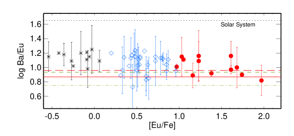
Figure 1: The Ba/Eu abundance ratios of the r-II (filled circles), r-I (open rombs), and Eu-poor (asterisks) stars (for the sources of the data, see text). The error bars were computed as $\sigma_{\rm Ba/Eu}=\sqrt{\sigma_{\rm Ba}^{2}+\sigma_{\rm Eu}^{2}}$, where the abundance errors available. The continuous and long-dashed lines indicate the SSr ratios, as predicted by GCE calculations of Bisterzo et al. (2014) and Travaglio et al. (1999), respectively, while the short-dashed and dash-dotted lines correspond to the SSr of Arlandini et al. (1999) and Bisterzo et al. (2011), respectively. The dotted line corresponds to the Solar System ratio (Lodders et al. 2009).

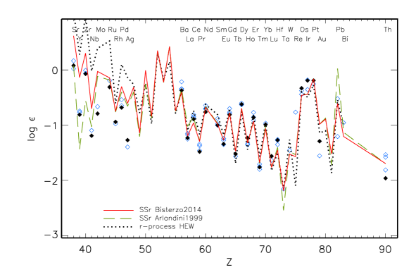
Figure 2: The heavy-element abundance patterns of CS 22892-052 (filled rombs) and the benchmark r-II stars CS 31082-001, HE 1523-0901, and HE 1219-0312 (open triangles). The element abundances have been scaled to match Eu–Tm in CS 22892-052. The dashed and continuous curves indicate the SSr abundance patterns calculated using the $s$-process predictions of A99 and B14, respectively. The dotted curve corresponds to the HEW $r$-process model of Farouqi et al. (2010).

This paper is structured as follows. In Sect. 2, we describe NLTE calculations for Ba ii and Eu ii in VMP atmospheres and evaluate the HFS effects on Ba abundance determinations. Abundances of Ba and Eu of the selected r-II stars are revised in Sect. 3. Section 4 summarizes the obtained results.

2 Method of calculations

2.1 NLTE modelling of Ba ii and Eu ii

In the NLTE calculations for Ba ii and Eu ii, we used model atoms treated in our earlier studies (Mashonkina et al. 1999, Mashonkina & Gehren 2000, updated). The coupled radiative transfer and statistical equilibrium (SE) equations were solved with a revised version of the DETAIL program (Butler & Giddings 1985), based on the accelerated lambda iteration method described by Rybicki & Hummer (1991, 1992). An update was presented by Mashonkina et al. (2011). The obtained level populations were then used to calculate spectral line profiles with the code SIU (Reetz 1991). We used classical plane-parallel (1D) models from the MARCS grid (Gustafsson et al. 2008).

Figure LABEL:Fig:bf displays the departure coefficients, $b_{i}=n_{i}^{\rm NLTE}/n_{i}^{\rm LTE}$, for the Ba ii and Eu ii levels in the model 4800/1.5/$-3.1$, representing the atmosphere of CS 22892-052 with effective temperature $T_{\mbox{\scriptsize eff}}$ = 4800 K, surface gravity log g = 1.5, and iron abundance [Fe/H] = $-3.1$. Here, $n_{i}^{\rm NLTE}$ and $n_{i}^{\rm LTE}$ are the SE and TE number densities, respectively. For both Ba ii and Eu ii, their ground states (denoted as 6s for Ba ii and 19S* for Eu ii) and low-excitation metastable levels (5d32 and 5d52 for Ba ii; 39D*, 59D*, 79D*, and 97D* for Eu ii) nearly keep TE level populations, with b $\simeq$ 1, throughout the atmosphere. This is because each of these ions contains the majority of its element. For Ba ii, the population of the upper level 6p (fine-splitting levels 6p12 and 6p32) of the resonance transition drops below its TE population in the atmospheric layers upwards of $\log\tau_{5000}=-1$, due to photon losses in the resonance lines themselves. The departures from LTE lead to strengthened resonance lines of Ba ii and negative NLTE abundance corrections $\Delta_{\rm NLTE}=\log\varepsilon_{\rm NLTE}-\log\varepsilon_{\rm LTE}$. For example, $\Delta_{\rm NLTE}$ = $-0.14$ dex for Ba ii 4554 Å. In the layers, where the weakest subordinate line Ba ii 5853 Å forms, b(6p) changes its magnitude from above 1 to below 1, resulting in small NLTE effects for the line, with $\Delta_{\rm NLTE}$ = $-0.02$ dex. For Eu ii, radiative pumping of the transitions from the ground state leads to overpopulation of the excited levels in the line-formation layers, resulting in weakened lines and positive NLTE abundance corrections. For example, $\Delta_{\rm NLTE}$ = 0.08 dex for Eu ii 4129 Å.

Table 2: Literature data on stellar parameters of the r-II stars and LTE abundances of Ba and Eu.

Star	$T_{\mbox{\scriptsize eff}}$	log g	[Fe/H]	$\xi_{t}$	Ba abundance				Eu abundance		Refs
	(K)			km s-1	$\log\varepsilon$	$f_{\rm odd}$	Comments		$\log\varepsilon$	N
CS 22183-031	5270	2.8	$-2.93$	1.2	$-0.33$	0.72	Ba ii 4554,4934Å		$-1.22$	3	1
CS 22892-052	4800	1.5	$-3.1$	1.95	0.02	0.52	Ba ii, 8 lines		$-0.95$	8	2
CS 22953-003	5100	2.3	$-2.84$	1.7	$-0.18$	0.52	Ba ii, 5 lines		$-1.27$	1	3
CS 29497-004	5090	2.4	$-2.64$	1.6	0.50	0.72	Ba ii 4554,4934Å		$-0.45$	2	4
CS 31078-018	5260	2.75	$-2.85$	1.5	$-0.06$	0.72	Ba ii 4554,4934,5853Å		$-1.17$	4	5
CS 31082-001	4825	1.5	$-2.9$	1.8	0.40	0.52	Ba ii, 6 lines		$-0.76$	9	6
HE 0432-0923	5130	2.64	$-3.19$	1.5	$-0.34$	0.72	Ba ii 4554Å		$-1.43$	2	7
HE 1219-0312	5060	2.3	$-2.96$	1.6	$-0.14$	0.72	Ba ii 4554,4934Å		$-1.06$	3	8
HE 1523-091	4630	1.0	$-2.95$	2.6	0.28	-	-		$-0.62$	-	9
HE 2224+0143	5200	2.66	$-2.58$	1.7	0.13	0.72	Ba ii 4554Å		$-1.02$	4	7
HE 2327-5642	5050	2.34	$-2.78$	1.8	$-0.30$	0.46	Ba ii 5853,6141,6496Å		$-1.29$	4	10
SDSS J2357-0052	5000	4.8	$-3.4$	0	$-0.10$	-	Ba ii 5853,6141,6496Å		$-0.92$	3	11
Refs: 1 = Honda et al. (2004); 2 = Sneden et al. (2003); 3 = François et al. (2007); 4 = Christlieb et al. (2004);
5 = Lai et al. (2008); 6 = Hill et al. (2002); 7 = Barklem et al. (2005); 8 = Hayek et al. (2009);
9 = Sneden et al. (2008); 10 = Mashonkina et al. (2010); 11 = Aoki et al. (2010).

The departures from LTE depend on stellar parameters and the line under investigation. Most r-II stars are VMP cool giants, with the exception of a VMP dwarf discovered by Aoki et al. (2010). Barium and europium are represented in their spectra mostly in the resonance and low-excitation lines of the majority species, Ba ii and Eu ii. We performed NLTE calculations for Ba ii and Eu ii in a grid of model atmospheres with $T_{\mbox{\scriptsize eff}}$ = 4500-5250 K, log g = 1.0-2.75 and log g = 4.8, [Fe/H] = $-3$ to $-2$, and element abundances characteristic of the r-II stars. In the SE computations, inelastic collisions with neutral hydrogen atoms were taken into account using the classical Drawin (1968, 1969) formalism with a scaling factor of $S_{\!\!\rm H}$ = 0.01 for Ba ii and $S_{\!\!\rm H}$ = 0.1 for Eu ii. This choice is based on our previous analyses of solar and stellar lines of these chemical species (Mashonkina & Gehren 2000). The investigated lines together with their atomic data are listed in Table 6 (online material). The results are presented as the LTE equivalent widths, EW (mÅ), and NLTE abundance corrections, $\Delta_{\rm NLTE}$, in Table LABEL:Tab:ba_nlte (online material) for lines of Ba ii and Table LABEL:Tab:eu_nlte (online material) for lines of Eu ii.

As expected, the NLTE effects for Ba ii and Eu ii are minor in the atmosphere of the VMP dwarf (5010/4.8/$-3.4$), with $\Delta_{\rm NLTE}\leq$ 0.03 dex in absolute value, and they grow towards lower gravity. For the VMP giant models, $\Delta_{\rm NLTE}$ is negative for the Ba ii 4554, 4934 Å resonance lines and low-excitation triplet lines at 5853, 6141, and 6496 Å. Positive NLTE corrections are predicted for the Ba ii 3891 and 4130 Å lines arising from the 6p sublevels. As shown in our previous study (Mashonkina et al. 1999), the departures from LTE for Ba ii depend on not only stellar parameters, but also the element abundance itself. As can be seen in Table LABEL:Tab:ba_nlte (online material), this effect is, in particular, notable for Ba ii 5853, 6141, 6496 Å. For example, in the model atmosphere 4800/1.5/$-3$, the NLTE corrections of these lines reduce by 0.11-0.13 dex, in absolute value, when moving to a 0.4 dex lower Ba abundance. For lines of Eu ii, $\Delta_{\rm NLTE}$ is positive and ranges between 0.03 and 0.2 dex.

2.2 HFS effects

Barium and europium are represented in nature by several isotopes (see Table 1 for isotopic abundances of the meteoritic matter). In the odd-atomic mass isotopes, nucleon-electron spin interactions lead to hyper-fine splitting of the energy levels, resulting in absorption lines divided into multiple components. The existence of isotopic splitting (IS) and/or HFS structure makes the line broader allowing more energy to be absorbed. Without accounting properly for IS and/or HFS structure, abundances determined from the lines sensitive to these effects can be severely overestimated.

Prominent Eu ii lines have very broad HFS and IS structure. For example, Eu ii 4129 Å consists of, in total, 32 components with 180 mÅ wide patterns. Accurate HFS data for lines of Eu ii were provided by Lawler et al. (2001). For the isotope abundance ratio ${}^{151}{\rm Eu}$ : ${}^{153}{\rm Eu}$, most studies of the r-II stars used either the meteoritic ratio 47.8 : 52.2 (Table 1) or 50 : 50. Both choices are justified, because a pure $r$-process Eu isotope mixture is expected to be very similar to the Solar System one, as shown in Table 3. Furthermore, there is observational evidence for equal abundance fractions of ${}^{151}{\rm Eu}$ and ${}^{153}{\rm Eu}$ in the VMP stars, including the r-II star CS 22892-052, as reported by Sneden et al. (2002). Therefore, Eu abundances of the r-II stars available in the literature do not need a revision for the HFS effect.

Table 3: Ba and Eu isotope abundance fractions (%) in the $r$-process.

	${}^{135}{\rm Ba}$	${}^{137}{\rm Ba}$	${}^{138}{\rm Ba}$			${}^{151}{\rm Eu}$	${}^{153}{\rm Eu}$
Sneden96	40.2	12	47.8			47	53
McW98	40	32	28			-	-
T99	24	22	54			47.4	52.6
B14	32	28.1	39.9			47.8	52.2
A99	26	20	54			47.4	52.6
B11	36.8	29.3	33.9			47.8	52.2
WP	29.2	14.6	56.2			-	-
Sneden96 = Sneden et al. (1996), McW98 = McWilliam (1998),
T99 = Travaglio et al. (1999), B14 = Bisterzo et al. (2014),
A99 = Arlandini et al. (1999), B11 = Bisterzo et al. (2011),
WP = Kratz et al. (2007, log nn = 25).

Barium is a different case. Its isotope mixture is very different in the SS matter and the $r$-process, and different studies predicted different isotope abundance fractions for pure $r$-process nucleosynthesis (Table 3). The subordinate lines of Ba ii including prominent 5853, 6141, and 6496 Å lines are almost free of HFS effects. According to our estimate for Ba ii 6496 Å in the 4500/1.5/$-3$ model with [Ba/Fe] = 1, neglecting HFS makes a difference in abundance of no more than 0.01 dex.

However, about half of the studies of the r-II stars are based on using the resonance lines of Ba ii, which are strongly affected by HFS. For example, Ba ii 4554 Å consists of 15 components spread over 58 mÅ. Three of them are produced by the even-A (relative atomic mass) isotopes, and the isotopic shifts are small, at the level of 1 mÅ (Kelly & Tomchuk 1964). Each of the two odd-A isotopes, ${}^{135}{\rm Ba}$ and ${}^{137}{\rm Ba}$, produce six HFS components disposed by two groups, very similarly for both isotopes. For Ba ii 4554 and 4934 Å, most abundance analyses are based on using the HFS patterns published by McWilliam (1998), which were calculated using the HFS constants from Brix & Kopfermann (1952). Having reviewed the literature for more recent data, Mashonkina et al. (1999) found that the use of new HFS constants of ${}^{135}{\rm Ba}$ and ${}^{137}{\rm Ba}$ from Blatt & Werth (1982) and Becker & Werth (1983) leads to a negligible change in the wavelength separations by no more than 1%  for the HFS components of Ba ii 4554 Å. In order to have common input data with other authors that makes a direct comparison of the results possible, in this study all calculations of the Ba ii resonance lines were performed using the wavelength separations and relative intensities of the components from McWilliam (1998). Table 4 illustrates the effect of using different Ba isotope mixtures on LTE and NLTE abundances derived from the Ba ii resonance lines in the r-II stars CS 22892-052 and CS 29497-004. The difference in NLTE abundance between using different predictions for the $r$-process can be up to 0.14 dex.

Table 4: Barium LTE and NLTE abundances, $\log\varepsilon$, of CS 22892-052 and CS 29497-004 for different Ba isotope mixtures.

$\lambda$	CS 22892-0521				CS 29497-0041
(Å)	EW2	LTE	NLTE3		LTE4	NLTE4,5
Ba isotopes:		solar mixture, L20096
Ba ii 45547	177	0.11	0.00		0.56	0.49
Ba ii 4934	180	0.33	0.06		0.94	0.63
	$r$-process, Sneden et al. (1996)
Ba ii 4554	177	$-$0.05	$-$0.18		0.47	0.36
Ba ii 4934	180	0.08	$-$0.22		0.75	0.35
	$r$-process, McWilliam (1998)
Ba ii 4554	177	$-$0.13	$-$0.28		0.42	0.29
Ba ii 4934	180	$-$0.02	$-$0.33		0.66	0.23
	$r$-process, Arlandini et al. (1999)
Ba ii 4554	177	$-$0.03	$-$0.17		0.48	0.37
Ba ii 4934	180	0.07	$-$0.19		0.56	0.29
mean		0.02	$-$0.18		0.52	0.33
	$r$-process, Bisterzo et al. (2011)
Ba ii 4554	177	$-$0.11	$-$0.26		0.43	0.31
Ba ii 4934	180	0.01	$-$0.30		0.68	0.26
mean		$-$0.05	$-$0.28		0.56	0.28
Ba ii 5853	72	$-$0.10	$-$0.13
Ba ii 6141	119	0.03	$-$0.17
Ba ii 6496	117	0.11	$-$0.16
mean		0.02	$-$0.15
		$\pm$0.11	$\pm$0.02
Notes. 1 Stellar parameters from Table 2,
2 equivalent widths (mÅ) from Sneden et al. (1996),
3 $\log\varepsilon_{\rm Ba}$ = $-0.11$ in the SE calculations,
4 from line profile fitting, 5 $\log\varepsilon_{\rm Ba}$ = 0.24 in the SE calculations,
6 Lodders et al. (2009),
7 line data from Table 6 (online material).

From observations, the total fractional abundance of ${}^{135}{\rm Ba}$ and ${}^{137}{\rm Ba}$, $f_{\mathrm{odd}}$, can only be derived because these isotopes have very similar HFS. In the SS matter, $f_{\mathrm{odd}}=0.18$. For the $r$-process, different studies predicted $f_{\mathrm{odd}}$ = 0.46 to 0.72 (Table 3). Stellar Ba isotopic fractions were determined in few studies. Magain & Zhao (1993) have suggested a method based on measuring the broadening of the Ba ii 4554 Å line in a very high-quality observed spectrum (resolving power $R=\lambda/\Delta\lambda\simeq 100\,000$ and signal-to-noise ratio $S/N\simeq 180$) of the nearby halo star HD 140283. Even higher $R$ and $S/N$ spectra of this star were then used by Magain (1995, $R\simeq 100\,000$, $S/N\simeq 400$), Lambert & Allende Prieto (2002, $R\simeq 200\,000$, $S/N\simeq 550$), and Gallagher et al. (2010, $S/N\simeq 1\,110$), but the obtained results were contrasting. Magain (1995) and Gallagher et al. (2010) found that the odd-A isotopes constitute a minor fraction of the total Ba in HD 140283, with $f_{\mathrm{odd}}$ = 0.08 and 0.02, respectively, suggesting a pure $s-$process production of barium. It is worth noting that Arlandini et al. (1999, stellar model) predicted $f_{\mathrm{odd}}^{s}=0.11$ for the $s-$process. Lambert & Allende Prieto (2002) obtained $f_{\mathrm{odd}}=0.30\pm 0.21$ which covers the full range of possibilities from a pure $s-$ to a pure $r-$process production of Ba. Completely disappointing results were presented by Gallagher et al. (2012) for three metal-poor stars, with $f_{\mathrm{odd}}$ = $-0.12\pm 0.07$, $-0.02\pm 0.09$, and $-0.05\pm 0.11$ for HD 122563, HD 88609, and HD 84937, respectively. The fractions $f_{\mathrm{odd}}$ = $0.08\pm 0.08$ and $0.18\pm 0.08$ measured in another two halo stars BD +26^∘3578 and BD$-04^{\circ}$3208 have, at least, a physical sense. Gallagher et al. (2012) concluded that “it is much more likely that the symmetric 1D LTE techniques used in this investigation are inadequate and improvements to isotopic ratio analysis need to be made.” The data cited above for HD 140283 were also based on a LTE analysis using 1D model atmospheres. The three-dimensional (3D) hydrodynamical model and LTE assumption were only applied by Collet et al. (2009). With the observed spectrum from Lambert & Allende Prieto (2002), they obtained $f_{\mathrm{odd}}=0.15\pm 0.12$ for HD140283.

A different method based on abundance comparisons between the subordinate and resonance lines of Ba ii was used in our earlier studies. The subordinate lines provide the total abundance of Ba in a star. The element abundance is then deduced from the resonance lines for various isotopic mixtures, the proportion of the odd isotopes being changed until agreement with the subordinate lines is obtained. Table 4 can serve to illustrate this method. For CS 22892-052, consistent abundances from different lines are achieved with $f_{\mathrm{odd}}\simeq 0.45$. However, one needs to be very cautious when applying such an approach to a star in which the resonance lines of Ba ii are saturated and very sensitive to variation in microturbulence velocity $\xi_{\rm t}$. For CS 22892-052, $\Delta\xi_{\rm t}=0.2$ km s^-1 produces a change in abundance of 0.15 dex that is comparable with the HFS effect. Taking advantage of NLTE line formation calculations of Ba ii, Mashonkina & Zhao (2006) and Mashonkina et al. (2008) derived $f_{\mathrm{odd}}$-values for three nearby halo stars and 15 thick disk stars with well determined stellar parameters. The two halo stars, HD 103095 ($f_{\mathrm{odd}}$ = 0.42$\pm$0.06) and HD 84937 ($f_{\mathrm{odd}}$ = 0.43$\pm$0.14), and the thick disk stars (the mean $f_{\mathrm{odd}}$ = 0.33$\pm$0.04) reveal higher fractions of the odd isotopes of Ba compared with that for the solar Ba isotope mixture. For HD 122563, the obtained $f_{\mathrm{odd}}$ = 0.22$\pm$0.15 is close to the SS one.

The observational evidence summarised above indicates that stellar $f_{\mathrm{odd}}$ is related to the $r$-process abundances of the star. Indeed, all the stars with high $f_{\mathrm{odd}}$-values, i.e., HD 103095, HD 84937, and the investigated thick disk stars, reveal an enhancement of europium relative to iron, with [Eu/Fe] = 0.24 to 0.70 (Mashonkina & Gehren 2001, Mashonkina et al. 2008). Analysis of the r-II star HE 2327-5642, with [Eu/Fe] = 0.98, also favored a high fraction of the odd isotopes of Ba, with $f_{\mathrm{odd}}\simeq 0.5$ (Mashonkina et al. 2010). In contrast, both stars with low $f_{\mathrm{odd}}$ are Eu-poor. For HD 122563, [Eu/Fe] = $-0.51$ / $-0.63$ (NLTE / LTE, Mashonkina et al. 2008), and only an upper limit, [Eu/Fe] $<-0.2$, was obtained for HD 140283 (Gallagher et al. 2010).

3 Barium and europium abundances of the r-II stars

In this study, the NLTE abundances of Ba and Eu were obtained for 8 of the 12 r-II stars currently known. HE 1523-091 was not included in our analysis, because there is no list of the used lines in Sneden et al. (2008). CS 31078-018 was not included, too, because we could not reproduce the LTE element abundances published by Lai et al. (2008), when employing their online material for observed equivalent widths of the Ba ii and Eu ii lines. We also did not use HE 0432-0923 and HE 2224+0143, with stellar parameters and element abundances based on an automated line profile analysis of moderate-resolution ($R\simeq$ 20 000) “snapshot” spectra (Paper II).

For the investigated stars, the NLTE calculations were performed with stellar parameters taken from the literature. They are listed in Table 2. The element abundances were derived using the line lists from the original papers. An exception is HE 1219-0312, where we employed an extended list of the Ba ii and Eu ii lines from Mashonkina et al. (2010). For the final abundances of Ba, we preferred to use the subordinate lines of Ba ii, which are nearly free of the HFS effects. In cases where only the resonance lines were available, homogeneous abundances were calculated using a common mixture of the Ba isotopes. Five different isotope mixtures were checked for CS 22892-052 and CS 29497-004 (Table 4) and two, as predicted by A99 (and also T99) and B11 for the $r$-process, for the remaining stars. For Eu in all the stars except CS 29497-004, HE 1219-0312, and HE 2327-5642, the NLTE calculations were performed with published LTE abundances, and the final NLTE abundances were obtained by applying the NLTE corrections. Table 5 presents the obtained results for the option of using the A99 (T99) $r$-process. Below, we comment on the individual stars.

Table 5: Obtained LTE and NLTE abundances, $\log\varepsilon$, and abundance ratios log(Ba/Eu) of the $r$-process enhanced stars.

	LTE				NLTE			Notes
Star	Ba	Eu	Ba/Eu		Ba	Eu	Ba/Eu
	Ba abundance from the Ba ii subordinate lines
CS 22892-052	0.02$\pm 0.11$	$-0.95$$\pm$0.03	0.97		$-0.15$$\pm$0.02	$-0.85$$\pm$0.03	0.70	(a)
HE 1219-0312	$-0.06$$\pm$0.03	$-0.99$$\pm$0.03	0.93		$-0.15$$\pm$0.10	$-0.88$$\pm$0.01	0.73	(b)
HE 2327-5642	$-0.30$$\pm$0.03	$-1.29$$\pm$0.02	0.99		$-0.30$$\pm$0.06	$-1.12$$\pm$0.04	0.82	(c)
SDSS J2357-0052	$-0.10$$\pm$0.09	$-0.92$$\pm$0.19	0.82		$-0.09$$\pm$0.09	$-0.89$$\pm$0.19	0.80	(d)
	Ba abundance from the subordinate and resonance lines, $f_{odd}=0.5$
CS 22953-003	$-0.22$	$-1.27$	1.05		$-0.23$	$-1.12$	0.89	(e)
CS 31082-001	0.39	$-0.76$$\pm$0.11	1.07		0.05	$-0.70$$\pm$0.11	0.75	(e)
	Ba abundance from the resonance lines, $f_{odd}=0.5$
CS 22183-031	$-0.21$$\pm$0.15	$-1.22$$\pm$0.08	1.01		$-0.35$$\pm$0.15	$-1.08$$\pm$0.08	0.73	(d)
CS 29497-004	0.50$\pm$0.06	$-0.54$$\pm$0.07	1.04		0.30$\pm$0.06	$-0.46$$\pm$0.05	0.76	(b)
mean			0.98				0.77
Notes. (a) Ba: EW, Sneden et al. (1996); Eu: $\Delta_{\rm NLTE}$, (b) syn, VLT/UVES spectrum,
(c) Mashonkina et al. (2010), (d) $\Delta_{\rm NLTE}$, (e) Ba: Andrievsky et al. (2009); Eu: $\Delta_{\rm NLTE}$.

CS 29497-004 and HE 1219-0312. The LTE and NLTE abundances of Ba and Eu were derived from line profile fitting of the UVES/VLT spectra taken from the original papers of Christlieb et al. (2004) and Hayek et al. (2009), respectively. For Ba in HE 1219-0312, the final abundance is based on the subordinate lines. The spectrum of CS 29497-004 did not cover the 5853-6496 Å range, and the Ba abundances were determined from the resonance lines for various isotope mixtures (Table 4).

CS 22892-052. For Ba, we used the equivalent widths published by Sneden et al. (1996) and the final abundance is based on the three subordinate lines (Table 4). We wish to note a dramatic reduction in the statistical abundance error from 0.11 to 0.02 dex, when moving from LTE to NLTE. This also holds for the two resonance lines. These results favor the NLTE line formation for Ba ii.

CS 22953-003 and CS 31082-001. The NLTE abundances of Ba were taken from Andrievsky et al. (2009), where they were derived from Ba ii 5853, 6496, and 4554 Å using $f_{\mathrm{odd}}=0.5$.

HE 2327-5642. The NLTE abundances of Ba and Eu were determined in our earlier study (Mashonkina et al. 2010), using only the Ba ii subordinate lines for Ba.

CS 22183-031 and SDSS J2357-0052. The NLTE abundances of Ba and Eu were calculated by applying NLTE corrections computed for individual spectral lines. SDSS J2357-0052 is the only dwarf among the r-II stars, and it reveals small departures from LTE. For CS 22183-031, the published LTE abundance of Ba (Table 2) was transformed to $f_{\mathrm{odd}}=0.5$ by adding a HFS correction of +0.12 dex.

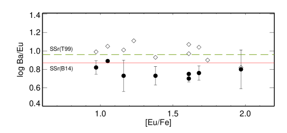
Figure 4: The LTE (rombs) and NLTE (filled circles) Ba/Eu abundance ratios of the r-II stars. The Ba abundance from the Ba ii resonance lines was derived using $f_{\mathrm{odd}}=0.5$. The continuous and dashed lines indicate the SSr ratios log(Ba/Eu)_r = 0.87 and 0.96, as predicted by B14 and T99

, respectively.

The obtained Ba/Eu abundance ratios are displayed in Fig. 4. In LTE, the mean from 10 stars is log(Ba/Eu) = 0.99$\pm$0.09. Here, we include CS 31078-018 and HE 1523-091, with the original LTE ratios log(Ba/Eu) = 1.11 (Lai et al. 2008) and 0.90 (Sneden et al. 2008). In NLTE, log(Ba/Eu) = 0.78$\pm$0.06 and 0.75$\pm$0.07 from 8 stars, when using the $r$-process Ba isotope mixtures from A99 (T99) and B11, respectively, for the four stars with Ba abundances determined from the Ba ii resonance lines. The NLTE Ba/Eu abundance ratios of the r-II stars support the recent predictions of Bisterzo et al. (2011) and Bisterzo et al. (2014) for the solar $r$-residuals and also the HEW $r$-process model of Farouqi et al. (2010).

In this study, we did not consider the effects on the Ba and Eu abundances of the use of 3D hydrodynamical model atmospheres. Both elements are observed in the r-II stars in the lines of their majority species, and the detected lines arise from either the ground or low-excitation levels. Dobrovolskas et al. (2013) predicted that the (3D-1D) abundance corrections are small and very similar in magnitude for the $E_{\rm exc}$ = 0 lines of Ba ii and Eu ii in the MP cool giant models. For example, (3D-1D) $=-0.05$ dex and $-0.04$ dex for the resonance lines of Ba ii and Eu ii, respectively, in the 5020/2.5/$-3$ model.

4 Conclusions

In this study, the Ba and Eu abundances of the eight r-II stars were revised by taking departures from LTE for lines of Ba ii and Eu ii into account, and accounting for HFS affecting the Ba ii resonance lines with a common Ba isotope mixture. For most of the r-II stars, NLTE leads to a lower Ba, but a higher Eu abundance. Therefore, the Ba/Eu abundance ratios decrease on average by 0.21 dex when moving from LTE to NLTE We conclude that an adequate line-formation modelling for heavy elements is important for abundance comparisons between VMP stars, and in particular, giants.

For stellar Ba abundance determinations, we recommend to use the subordinate lines of Ba ii, which are nearly free of the HFS effects. At present, there is no consensus on the Ba isotope abundance fractions in the $r$-process, and abundances derived from the Ba ii resonance lines vary by 0.15 dex, when applying different $r$-process models. We suspect that the total fractional abundance of the odd-A isotopes of Ba in old Galactic stars is related to the $r$-process abundances of the star. The observational evidence indicates that all the stars with high $f_{\mathrm{odd}}$-values, i.e., HD 103095, HD 84937, HE 2327-5642, and the selected thick disk stars, are $r$-process enhanced, with [Eu/Fe] = 0.24 to 0.70 (Mashonkina & Zhao 2006, Mashonkina et al. 2008, 2010). In contrast, both stars with low $f_{\mathrm{odd}}$, i.e., HD 122563 and HD 140283, are Eu-poor, with [Eu/Fe] = $-0.51$ (Mashonkina et al. 2008, NLTE) and [Eu/Fe] $<-0.2$ (Gallagher et al. 2010), respectively.

With the improved Ba and Eu abundances of the r-II stars, we constrain a pure $r$-process Ba/Eu abundance ratio to be log(Ba/Eu)_r = 0.78$\pm$0.06. The obtained results support the solar $r$-residuals based on the chemical evolution calculations of Bisterzo et al. (2011) and Bisterzo et al. (2014), and also the HEW $r$-process model by Farouqi et al. (2010).

For further constraining the $r$-process models, it would be important to determine Ba isotopic fractions of the r-II stars. This is a challenge for theory as well as observations.

Table 6: Atomic data for the investigated lines. $\Gamma_{6}$ corresponds to 10 000 K. References to the adopted $gf-$values and $\Gamma_{6}-$values are given in column 4 and 6, respectively.

$\lambda$(Å)	$E_{\rm exc}$(eV)	log $gf$	Refs	log$\Gamma_{6}$	Refs
Ba ii 3891.78	2.51	0.28	1	$-$7.870	3
Ba ii 4130.64	2.72	0.56	1	$-$7.870	3
Ba ii 4554.03	0.00	0.17	1	$-$7.732	4
Ba ii 4934.08	0.00	$-$0.15	1	$-$7.732	4
Ba ii 5853.67	0.60	$-$1.01	1	$-$7.584	5
Ba ii 6141.71	0.70	$-$0.07	1	$-$7.584	5
Ba ii 6496.90	0.60	$-$0.38	1	$-$7.584	5
Eu ii 3724.93	0.00	$-$0.09	2	$-$7.870	3
Eu ii 3819.67	0.00	0.51	2	$-$7.870	3
Eu ii 3907.11	0.21	0.17	2	$-$7.870	3
Eu ii 3930.50	0.21	0.27	2	$-$7.870	3
Eu ii 3971.97	0.21	0.27	2	$-$7.870	3
Eu ii 4129.72	0.00	0.22	2	$-$7.870	3
Eu ii 4205.02	0.00	0.21	2	$-$7.870	3
Eu ii 4435.58	0.21	$-$0.11	2	$-$7.870	3
Eu ii 4522.58	0.21	$-$0.67	2	$-$7.870	3
Eu ii 6645.10	1.38	0.12	2	$-$7.870	3
Refs. 1 = Gallagher (1967), 2 = Lawler et al. (2001),
3 = adopted in this study, 4 = Mashonkina & Zhao (2006),
5 = Barklem & O’Mara (1998).

Table 7: Equivalent widths, EW_LTE(mÅ), and NLTE abundance corrections, $\Delta_{\rm NLTE}$(dex), for lines of Ba ii in the metal-poor model atmospheres. All the computations were performed with $\xi_{\rm t}$ = 1.8 km s^-1 except for the log g = 4.8 model, where $\xi_{\rm t}$ = 0 was adopted. Everywhere, $S_{\!\!\rm H}$ = 0.01. For line data, see Table 6. Lines with EW $<$ 5 mÅ are not shown.

Model	[Ba/Fe]		Ba ii lines, $\lambda$(Å)
			4554	4934	5853	6141	6496	4130	3891
4500/1.00/$-$3.00	1.0	EWLTE	237	223	106	149	144	28	28
		$\Delta_{\rm NLTE}$	$-$0.03	$-$0.09	$-$0.13	$-$0.17	$-$0.24	0.41	0.34
4500/1.00/$-$3.00	0.5	EWLTE	187	183	79	119	114	12	12
		$\Delta_{\rm NLTE}$	$-$0.04	$-$0.14	$-$0.04	$-$0.13	$-$0.19	0.33	0.29
4500/1.00/$-$3.00	0.0	EWLTE	153	152	50	92	86
		$\Delta_{\rm NLTE}$	$-$0.03	$-$0.11	0.04	$-$0.01	$-$0.06
4500/1.50/$-$3.00	1.0	EWLTE	231	215	99	141	135	22	22
		$\Delta_{\rm NLTE}$	$-$0.04	$-$0.12	$-$0.13	$-$0.20	$-$0.26	0.31	0.26
4500/1.50/$-$3.00	0.5	EWLTE	179	174	71	111	105	8	8
		$\Delta_{\rm NLTE}$	$-$0.06	$-$0.16	$-$0.03	$-$0.13	$-$0.18	0.26	0.23
4500/1.50/$-$3.00	0.0	EWLTE	145	143	41	83	77
		$\Delta_{\rm NLTE}$	$-$0.04	$-$0.11	0.04	0.00	$-$0.04
4500/2.00/$-$3.00	1.0	EWLTE	230	210	92	135	127	16	16
		$\Delta_{\rm NLTE}$	$-$0.05	$-$0.13	$-$0.10	$-$0.19	$-$0.24	0.24	0.20
4500/2.00/$-$3.00	0.5	EWLTE	174	167	61	103	96	6	6
		$\Delta_{\rm NLTE}$	$-$0.07	$-$0.16	$-$0.01	$-$0.11	$-$0.15	0.22	0.19
4500/2.00/$-$3.00	0.0	EWLTE	138	134	32	74	66
		$\Delta_{\rm NLTE}$	$-$0.04	$-$0.09	0.04	0.01	$-$0.02
4750/1.00/$-$3.00	1.0	EWLTE	201	193	94	132	127	26	25
		$\Delta_{\rm NLTE}$	$-$0.11	$-$0.24	$-$0.13	$-$0.27	$-$0.33	0.34	0.29
4750/1.00/$-$3.00	0.5	EWLTE	165	163	69	107	101	10	10
		$\Delta_{\rm NLTE}$	$-$0.12	$-$0.23	$-$0.01	$-$0.14	$-$0.19	0.28	0.25
4750/1.00/$-$3.00	0.0	EWLTE	138	137	39	82	75
		$\Delta_{\rm NLTE}$	$-$0.08	$-$0.12	0.07	0.01	$-$0.01
4750/1.50/$-$3.00	1.0	EWLTE	193	185	86	123	117	20	19
		$\Delta_{\rm NLTE}$	$-$0.13	$-$0.27	$-$0.12	$-$0.28	$-$0.33	0.28	0.24
4750/1.50/$-$3.00	0.5	EWLTE	157	155	59	98	92	8	7
		$\Delta_{\rm NLTE}$	$-$0.14	$-$0.23	0.00	$-$0.14	$-$0.17	0.24	0.21
4750/1.50/$-$3.00	0.0	EWLTE	130	128	31	73	65
		$\Delta_{\rm NLTE}$	$-$0.08	$-$0.11	0.06	0.02	0.00
4750/2.00/$-$3.00	1.0	EWLTE	189	179	79	117	110	15	14
		$\Delta_{\rm NLTE}$	$-$0.13	$-$0.26	$-$0.10	$-$0.26	$-$0.30	0.23	0.20
4750/2.00/$-$3.00	0.5	EWLTE	151	147	50	90	84	5	5
		$\Delta_{\rm NLTE}$	$-$0.14	$-$0.22	0.00	$-$0.12	$-$0.14	0.21	0.19
4750/2.00/$-$3.00	0.0	EWLTE	124	119	24	64	55
		$\Delta_{\rm NLTE}$	$-$0.07	$-$0.09	0.05	0.03	0.01
5000/2.00/$-$3.00	1.0	EWLTE	165	160	68	104	97	13	12
		$\Delta_{\rm NLTE}$	$-$0.17	$-$0.29	$-$0.05	$-$0.24	$-$0.27	0.23	0.20
5000/2.00/$-$3.00	0.5	EWLTE	136	133	39	80	72	5
		$\Delta_{\rm NLTE}$	$-$0.13	$-$0.17	0.05	$-$0.05	$-$0.06	0.22
5000/2.00/$-$3.00	0.0	EWLTE	112	106	17	53	44
		$\Delta_{\rm NLTE}$	$-$0.01	0.00	0.09	0.09	0.08
5000/2.50/$-$3.00	1.0	EWLTE	160	154	59	97	90	10	9
		$\Delta_{\rm NLTE}$	$-$0.16	$-$0.26	$-$0.03	$-$0.20	$-$0.22	0.22	0.19
5000/2.50/$-$3.00	0.5	EWLTE	130	125	31	72	63
		$\Delta_{\rm NLTE}$	$-$0.11	$-$0.13	0.04	$-$0.03	$-$0.04
5000/2.50/$-$3.00	0.0	EWLTE	104	96	12	43	35
		$\Delta_{\rm NLTE}$	0.01	0.02	0.08	0.09	0.07
4500/1.00/$-$2.00	0.5	EWLTE	284	260	125	174	167	46	46
		$\Delta_{\rm NLTE}$	$-$0.01	$-$0.05	$-$0.12	$-$0.12	$-$0.17	0.30	0.25
4500/1.00/$-$2.00	0.5	EWLTE	216	208	98	140	134	24	23
		$\Delta_{\rm NLTE}$	$-$0.03	$-$0.08	$-$0.09	$-$0.14	$-$0.18	0.27	0.23
4500/1.50/$-$2.00	0.5	EWLTE	267	244	115	161	154	38	37
		$\Delta_{\rm NLTE}$	$-$0.03	$-$0.07	$-$0.14	$-$0.16	$-$0.21	0.25	0.20
4500/1.50/$-$2.00	0.0	EWLTE	203	196	87	128	122	18	17
		$\Delta_{\rm NLTE}$	$-$0.04	$-$0.11	$-$0.08	$-$0.16	$-$0.19	0.21	0.18
4500/2.00/$-$2.00	0.5	EWLTE	257	233	105	151	142	30	29
		$\Delta_{\rm NLTE}$	$-$0.04	$-$0.08	$-$0.12	$-$0.17	$-$0.21	0.20	0.16
4500/2.00/$-$2.00	0.0	EWLTE	194	185	77	117	110	12	12
		$\Delta_{\rm NLTE}$	$-$0.05	$-$0.12	$-$0.05	$-$0.15	$-$0.17	0.17	0.14
4750/1.00/$-$2.00	0.5	EWLTE	254	237	117	162	155	47	45
		$\Delta_{\rm NLTE}$	$-$0.04	$-$0.09	$-$0.17	$-$0.20	$-$0.27	0.32	0.27
4750/1.00/$-$2.00	0.0	EWLTE	199	194	92	131	126	24	23
		$\Delta_{\rm NLTE}$	$-$0.06	$-$0.15	$-$0.09	$-$0.20	$-$0.25	0.27	0.24
4750/1.50/$-$2.00	0.5	EWLTE	239	223	108	150	143	39	37
		$\Delta_{\rm NLTE}$	$-$0.05	$-$0.13	$-$0.17	$-$0.24	$-$0.29	0.27	0.22
4750/1.50/$-$2.00	0.0	EWLTE	188	183	82	120	114	18	17
		$\Delta_{\rm NLTE}$	$-$0.08	$-$0.18	$-$0.08	$-$0.20	$-$0.24	0.22	0.19
4750/2.00/$-$2.00	0.5	EWLTE	229	212	99	141	133	31	29
		$\Delta_{\rm NLTE}$	$-$0.07	$-$0.14	$-$0.15	$-$0.24	$-$0.28	0.22	0.17
4750/2.00/$-$2.00	0.0	EWLTE	178	173	71	110	104	13	12
		$\Delta_{\rm NLTE}$	$-$0.09	$-$0.18	$-$0.06	$-$0.18	$-$0.21	0.18	0.16
5000/2.00/$-$2.00	0.5	EWLTE	202	191	91	128	122	30	28
		$\Delta_{\rm NLTE}$	$-$0.12	$-$0.25	$-$0.16	$-$0.31	$-$0.35	0.24	0.19
5000/2.00/$-$2.00	0.0	EWLTE	162	159	64	102	95	12	11
		$\Delta_{\rm NLTE}$	$-$0.14	$-$0.24	$-$0.04	$-$0.19	$-$0.22	0.20	0.18
5000/2.50/$-$2.00	0.5	EWLTE	196	184	82	121	114	23	21
		$\Delta_{\rm NLTE}$	$-$0.12	$-$0.23	$-$0.12	$-$0.27	$-$0.30	0.20	0.17
5000/2.50/$-$2.00	0.0	EWLTE	155	151	54	94	86	9	8
		$\Delta_{\rm NLTE}$	$-$0.13	$-$0.20	$-$0.02	$-$0.15	$-$0.17	0.18	0.16
4800/1.50/$-$3.00	1.1	EWLTE	199	189	90	127	121	24	23
		$\Delta_{\rm NLTE}$	$-$0.13	$-$0.26	$-$0.14	$-$0.30	$-$0.35	0.29	0.24
4800/1.50/$-$3.00	0.7	EWLTE	167	163	69	106	100	11	11
		$\Delta_{\rm NLTE}$	$-$0.14	$-$0.26	$-$0.03	$-$0.19	$-$0.23	0.25	0.23
5010/4.80/$-$3.40	1.1	EWLTE	100	82	8	32	25
		$\Delta_{\rm NLTE}$	$-$0.01	$-$0.01	0.01	0.01	0.01
5050/2.34/$-$2.84	1.0	EWLTE	169	161	67	103	96	14	13
		$\Delta_{\rm NLTE}$	$-$0.17	$-$0.30	$-$0.08	$-$0.28	$-$0.30	0.24	0.21
5050/2.34/$-$2.84	0.5	EWLTE	136	132	39	78	71	5	5
		$\Delta_{\rm NLTE}$	$-$0.15	$-$0.20	0.03	$-$0.09	$-$0.10	0.24	0.21
5260/2.75/$-$2.85	0.6	EWLTE	126	121	30	70	61
		$\Delta_{\rm NLTE}$	$-$0.13	$-$0.15	0.04	$-$0.04	$-$0.05
5260/2.75/$-$2.85	0.3	EWLTE	111	104	17	53	44
		$\Delta_{\rm NLTE}$	$-$0.04	$-$0.03	0.08	0.05	0.04

Table 7: continued.

Table 8: The same as in Table LABEL:Tab:ba_nlte for lines of Eu ii. Everywhere, $S_{\!\!\rm H}$ = 0.1.

Model	[Eu/Fe]		Eu ii lines, $\lambda$(Å)
			4129	4205	3819	3724	3907	4435	4522	3971	3930	6645
4500/1.00/$-$3.00	1.5	EWLTE	183	132	176	81	128	100	39	75	74	16
		$\Delta_{\rm NLTE}$	0.08	0.06	0.06	0.07	0.18	0.08	0.05	0.09	0.09	0.10
4500/1.00/$-$3.00	0.7	EWLTE	56	39	79	21	43	24	7	42	41
		$\Delta_{\rm NLTE}$	0.17	0.13	0.16	0.16	0.31	0.18	0.14	0.27	0.27
4500/1.50/$-$3.00	1.5	EWLTE	158	113	166	65	114	80	29	69	69	11
		$\Delta_{\rm NLTE}$	0.07	0.05	0.06	0.07	0.14	0.07	0.05	0.10	0.10	0.10
4500/1.50/$-$3.00	0.7	EWLTE	40	28	62	14	32	17	5	34	33
		$\Delta_{\rm NLTE}$	0.15	0.12	0.14	0.15	0.24	0.16	0.13	0.24	0.23
4500/2.00/$-$3.00	1.5	EWLTE	129	91	152	49	95	60	20	63	63	8
		$\Delta_{\rm NLTE}$	0.06	0.05	0.05	0.06	0.11	0.07	0.05	0.11	0.11	0.11
4500/2.00/$-$3.00	0.7	EWLTE	28	19	46	9	22	11		26	26
		$\Delta_{\rm NLTE}$	0.13	0.11	0.12	0.13	0.19	0.15		0.19	0.19
4750/1.00/$-$3.00	1.5	EWLTE	150	107	161	61	110	76	27	68	68	12
		$\Delta_{\rm NLTE}$	0.09	0.07	0.08	0.09	0.21	0.09	0.07	0.15	0.15	0.12
4750/1.00/$-$3.00	0.7	EWLTE	37	26	58	13	30	16	5	33	32
		$\Delta_{\rm NLTE}$	0.18	0.15	0.18	0.19	0.28	0.18	0.15	0.28	0.28
4750/1.50/$-$3.00	1.5	EWLTE	122	86	145	46	92	58	19	62	62	9
		$\Delta_{\rm NLTE}$	0.08	0.06	0.07	0.09	0.17	0.09	0.07	0.16	0.16	0.14
4750/1.50/$-$3.00	0.7	EWLTE	26	18	44	9	21	11		25	25
		$\Delta_{\rm NLTE}$	0.15	0.13	0.16	0.17	0.23	0.17		0.24	0.24
4750/2.00/$-$3.00	1.5	EWLTE	95	67	126	34	74	43	14	55	55	6
		$\Delta_{\rm NLTE}$	0.08	0.06	0.06	0.08	0.14	0.09	0.07	0.16	0.16	0.16
4750/2.00/$-$3.00	0.7	EWLTE	18	13	32	6	15	8		19	19
		$\Delta_{\rm NLTE}$	0.13	0.12	0.14	0.15	0.19	0.16		0.20	0.20
5000/2.00/$-$3.00	1.5	EWLTE	66	46	98	23	54	29	9	47	46	5
		$\Delta_{\rm NLTE}$	0.09	0.08	0.09	0.11	0.16	0.11	0.09	0.19	0.19	0.23
5000/2.00/$-$3.00	0.7	EWLTE	12	8	21		10	5		14	13
		$\Delta_{\rm NLTE}$	0.14	0.13	0.16		0.19	0.16		0.20	0.20
5000/2.50/$-$3.00	1.5	EWLTE	47	33	76	16	39	21	6	39	38
		$\Delta_{\rm NLTE}$	0.09	0.08	0.08	0.10	0.13	0.10	0.09	0.17	0.17
5000/2.50/$-$3.00	0.7	EWLTE	8	6	15		7			10	10
		$\Delta_{\rm NLTE}$	0.12	0.12	0.14		0.16			0.17	0.17
4500/1.00/$-$2.00	0.7	EWLTE	193	139	186	85	136	107	43	78	77	17
		$\Delta_{\rm NLTE}$	0.06	0.04	0.05	0.04	0.14	0.06	0.03	0.05	0.05	0.07
4500/1.50/$-$2.00	0.7	EWLTE	161	115	169	65	116	81	29	71	70	12
		$\Delta_{\rm NLTE}$	0.06	0.04	0.05	0.04	0.12	0.06	0.03	0.06	0.06	0.08
4500/2.00/$-$2.00	0.7	EWLTE	125	88	148	47	93	58	19	63	63	8
		$\Delta_{\rm NLTE}$	0.06	0.04	0.04	0.04	0.10	0.06	0.04	0.08	0.08	0.09
4750/1.00/$-$2.00	0.7	EWLTE	176	126	181	73	128	93	34	73	73	16
		$\Delta_{\rm NLTE}$	0.07	0.04	0.06	0.05	0.17	0.07	0.03	0.07	0.07	0.09
4750/1.50/$-$2.00	0.7	EWLTE	141	100	161	55	106	69	24	67	66	11
		$\Delta_{\rm NLTE}$	0.07	0.04	0.06	0.05	0.14	0.07	0.04	0.08	0.08	0.10
4750/2.00/$-$2.00	0.7	EWLTE	106	75	137	38	82	49	16	59	59	7
		$\Delta_{\rm NLTE}$	0.07	0.04	0.05	0.05	0.12	0.07	0.05	0.10	0.10	0.12
5000/2.00/$-$2.00	0.7	EWLTE	84	59	119	29	68	38	12	53	53	6
		$\Delta_{\rm NLTE}$	0.08	0.05	0.07	0.07	0.14	0.09	0.06	0.13	0.13	0.16
5000/2.50/$-$2.00	0.7	EWLTE	59	41	92	20	49	26	8	44	44
		$\Delta_{\rm NLTE}$	0.08	0.06	0.06	0.07	0.12	0.09	0.06	0.12	0.12
4800/1.50/$-$3.00	1.5	EWLTE	117	83	142	44	89	56	18	61	61	9
		$\Delta_{\rm NLTE}$	0.09	0.07	0.08	0.09	0.18	0.09	0.07	0.17	0.17	0.15
5010/4.80/$-$3.40	1.9	EWLTE	6		11		5			7	7
		$\Delta_{\rm NLTE}$	0.03		0.03		0.04			0.05	0.05
5050/2.34/$-$2.84	1.0	EWLTE	23	16	40	8	20	10		24	23
		$\Delta_{\rm NLTE}$	0.13	0.12	0.14	0.14	0.18	0.14		0.18	0.18
5260/2.75/$-$2.85	1.1	EWLTE	14	10	26	5	12	6		17	16
		$\Delta_{\rm NLTE}$	0.12	0.11	0.12	0.13	0.15	0.13		0.17	0.17

Table 8: continued.