Models of force-free spheres and applications
to solar active regions

Abstract

Here we present a systematic study of force-free field equation for simple axisymmetric configurations in spherical geometry. The condition of separability of solutions in radial and angular variables leads to two classes of solutions: linear and non-linear force-free fields. We have studied these linear solutions (Chandrasekhar, 1956) and extended the non-linear solutions given in Low & Lou (1990) to the irreducible rational form $n=p/q$, which is allowed for all cases of odd $p$ and to cases of $q>p$ for even $p$. We have further calculated their energies and relative helicities for magnetic field configurations in finite and infinite shell geometries. We demonstrate here a method here to be used to fit observed magnetograms as well as to provide good exact input fields for testing other numerical codes used in reconstruction on the non-linear force-free fields.

1 Introduction

In systems dominated by magnetic fields in the presence of kinematic viscosity, linear force-free fields are the natural end states. More general force-free fields can be obtained when the constraints of total mass, angular momentum and helicity are put in the equations, (e.g. Finn & Antonsen, 1983; Mangalam & Krishan, 2000). There have been several attempts to numerically construct the full three dimensional models of coronal fields from two dimensional three component data available from the vector magnetograms. Some of the popular techniques include Optimization (Wheatland et al.,2000; Wiegelmann, 2004) Magnetofrictional (Yang et. al., 1986; McClymont et. al., 1997), Grad-Rubin based (Amari et al., 2006; Wheatland $\&$ Leka, 2010), and Green’s function-based methods (Yan $\&$ Sakurai, 2000). We construct analytical models of linear and non-linear axisymmetric force-free fields by solving the governing equations. We then take a cross-section of these 3D fields at different orientations to construct a library of template magnetograms corresponding to the different modes of our solutions which can be then compared with the observed magnetograms to pick out the best fit. We apply the techniques outlined here to magnetograms and reconstruct the coronal fields in Prasad, Mangalam & Ravindra (2014, in press, henceforth referred to as PMR14), which also contains details of the formulation presented below.

2 Axisymmetric separable linear & non-linear force-free fields

The force-free magnetic field $\mathbf{B}$ is described by the equation $\nabla\times\mathbf{B}=\alpha\mathbf{B}$ An axisymmetric magnetic field can be expressed in terms of two scalar functions $\psi$ and $Q$ in spherical polar coordinates :

$$\mathbf{B}=\frac{1}{r\sin\theta}\left(\frac{1}{r}\frac{\partial\psi}{\partial\theta}\hat{\mathbf{r}}-\frac{\partial\psi}{\partial r}\hat{\boldsymbol{\theta}}+Q\hat{\boldsymbol{\phi}}\right).$$ (1)

We try separable solutions of the form $\psi=f(r)P(\mu),\quad Q=a\psi^{\beta}.$ which yields

$$r^{2}\frac{f^{\prime\prime}}{f}+(1-\mu^{2})\frac{P^{\prime\prime}}{P}+a^{2}\beta r^{2}f^{2\beta-2}P^{2\beta-2}=0.$$ (2)

There are two possibilities for getting separable solutions. The third term can be a function of

1. $r$ alone, which is satisfied if $\beta=1$; these solutions were presented in Chandrasekhar (1956) and which we refer to as C modes or

2. $\mu$ alone, which is satisfied if $r^{2}f^{2\beta-2}=1$; these solutions were partially explored by Low & Lou (1990) and termed here as LL modes.

Free energy and relative helicity are very helpful quantities for studying the dynamics of the magnetic field configurations near active regions in the Sun. The free energy of the system is the difference between the energies of a force-free field and a potential field in a volume. The potential field is constructed using the normal components of the force-free field at the boundary. The expression for free energy $E_{free}$ is given by $E_{free}=E_{ff}-E_{P},$

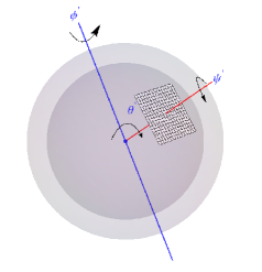
Figure 1: The left figure shows the geometry of the problem. The force-free field is first computed in the entire region (I and II) and then corresponding potential field is constructed in the spherical shell between radii $r_{1}$ and $r_{2}$ (region II) using the normal components of the force-free field at the lower boundary, $r_{1}$. The right figure shows a magnetogram which is simulated by taking a cross-section of the axisymmetric 3D force-free field at a radius $r_{1}$.The magnetogram is then rotated through the Euler angles $\theta^{\prime}$ and $\psi^{\prime}$ to match the components of the observed magnetogram. The rotation $\phi^{\prime}$ is redundant as the field is axisymmetric.

We model the force-free field using both the linear solutions (C modes) and the non-linear solutions (LL modes). where $E_{ff}$ and $E_{P}$ are the energies of the force-free field and the potential field respectively. Since the potential field is the minimum energy configuration for a given boundary condition, $E_{free}$ is always positive. Here we are modeling the entire active region as as a part of a force-free sphere with an inner radius $r_{1}$; where the magnetogram measurements are available and an outer radius $r_{2}$ as shown in the left panel of Fig.1.

C modes: with the condition $\beta=1$, we get $\displaystyle{r^{2}\frac{f^{\prime\prime}}{f}+a^{2}r^{2}=n(n+1)}$ as the equation for the radial part where $n$ is a constant, the solution to which is given by

$$f_{n}(r)=c_{1}\sqrt{r}J\left[(1+2n)/2,ar\right]+c_{2}\sqrt{r}Y\left[(1+2n)/2,ar\right].$$ (3)

The angular part is given by the following equation $(1-\mu^{2})\frac{P^{\prime\prime}}{P}=-n(n+1)$ whose solution is given by $P(\mu)=(1-\mu^{2})^{1/2}P_{n}^{1}(\mu).$ LL modes: the second condition $r^{2}f^{2\beta-2}=1$ implies $\beta=(n+1)/n$ for the functional form $f(r)=r^{-n},$ The differential equation for the angular part then becomes

$$(1-\mu^{2})\frac{P^{\prime\prime}}{P}+a^{2}\frac{n+1}{n}P^{1+2/n}+n(n+1)P=0.$$ (4)

The above equation is solved numerically as no general closed form is known for all values of $n$. For a given value of $n$, we get different modes for different eigenvalues of $a_{n,m}$ satisfying the above equation for a given boundary condition. Low $\&$ Lou(1990) were able to solve the above equation only for $n=1$ due to singular nature of the solutions. We were able to tackle this problem for higher values of $n$ through the transformation $P(\mu)=(1-\mu^{2})^{1/2}F(\mu),$ by which eqn (4) now stand as

$$(1-\mu^{2})F^{\prime\prime}(\mu)-2\mu F^{\prime}(\mu)+\left[n(n+1)-\frac{1}{(1-\mu^{2})}\right]F(\mu)+a^{2}\frac{(n+1)}{n}F^{\frac{(n+2)}{n}}(1-\mu^{2})^{\frac{1}{n}}=0.$$ (5)

We were able to obtain an infinite set of solutions for all rational values of $n=\displaystyle{\frac{p}{q}}$. For even values $p$, solutions exist if $F(\mu)>0$ in the domain $-1\leq\mu\leq 1$. In this case we get $\displaystyle{\alpha=\frac{a(1+1/n)(1-\mu^{2})^{1/2n}F^{1/n}}{r^{n}}.}$ The physical quantities of interest such as the force-free energy, free energy, $E_{ff}$, $E_{free}$ and the relative helicity $H_{rel}$ are calculated for the region above the magnetogram. The formulary of the results for the C and LL modes are presented in Table 1. The details of derivation are presented in PMR14.

C modes

$\mathbf{B}(r<r_{2})=\left(-\frac{1}{r^{2}}\frac{\partial}{\partial\mu}[S_{m}r^{2}(1-\mu^{2})],\frac{-1}{r\sqrt{(1-\mu^{2})}}\frac{\partial}{\partial r}[S_{m}r^{2}(1-\mu^{2})],\alpha r\sqrt{(1-\mu^{2})}S_{m}\right);\mathbf{A}(r<r_{2})=\mathbf{B}/\alpha$

$\chi_{m+1}(r_{1})=\frac{(m+1)(m+2)}{r_{1}^{3/2}}J_{m+3/2}(\alpha r_{1});a_{m+1}=\frac{\chi_{m+1}(r_{1})}{(m+1)}\frac{r_{1}^{m+3}}{r_{1}^{2m+3}-r_{2}^{2m+3}};b_{m+1}=\frac{(m+1)}{(m+2)}a_{m+1}r_{2}^{(2m+3)}$

$\mathbf{B}_{P}(r_{1}<r<r_{2})=\left(\left[(m+1)a_{m+1}r^{m}-\frac{(m+2)b_{m+1}}{r^{m+3}}\right]P_{m+1}(\mu),\right.\left.-(1-\mu^{2})^{1/2}\left[a_{m+1}r^{m}+\frac{b_{m+1}}{r^{m+3}}\right]\frac{\partial P_{m+1}}{\partial\mu},0\right)$

$\mathbf{A}_{P}(r_{1}<r<r_{2})=\left(0,0,(1-\mu^{2})^{1/2}P^{\prime}_{l}(\mu)\left[\frac{a_{l}r^{l}}{l+1}-\frac{b_{l}}{lr^{l+1}}\right]\right)$

$E_{ff}(\alpha,n,m,r_{1},r_{2})=\frac{(m+1)(m+2)}{2(2m+3)}\Bigl{[}(m+1)(m+2)\int_{r_{1}}^{r_{2}}\frac{J^{2}_{m+3/2}(\alpha r)}{r}\textrm{d}r+r^{3/2}J_{m+3/2}(\alpha r)|^{r_{1}}_{r_{2}}$

$~{}~{}~{}~{}~{}~{}~{}~{}~{}~{}~{}~{}~{}~{}~{}~{}~{}~{}~{}~{}~{}~{}~{}~{}~{}~{}~{}~{}-\int_{r_{1}}^{r_{2}}r^{1/2}J_{m+3/2}(\alpha r)\textrm{d}r+\alpha^{2}\int_{r_{1}}^{r_{2}}rJ^{2}_{m+3/2}(\alpha r)\textrm{d}r\Bigr{]}$

$E_{pot}(m,r_{1},r_{2})=\frac{1}{2(2m+3)}\int_{r_{1}}^{r_{2}}\Bigl{[}\left((m+1)a_{m+1}r^{m+1}-\frac{(m+2)b_{m+1}}{r^{m+2}}\right)^{2}$

$~{}~{}~{}~{}~{}~{}~{}~{}~{}~{}~{}~{}~{}~{}~{}~{}~{}~{}~{}+(m+1)(m+2)\left(a_{m+1}r^{m+1}+\frac{b_{m+1}}{r^{m+2}}\right)^{2}\Bigr{]}\textrm{d}r$

$H_{rel}(\alpha,n,m,r_{1},r_{2})=\frac{E_{ff}(\alpha,n,m)}{\alpha}+{1\over\alpha}\Bigl{[}\frac{2(m+1)(m+2)}{(2m+3)}\Bigl{[}\left(a_{m+1}r^{m+1}+\frac{b_{m+1}}{r^{m+2}}\right)\left(r^{1/2}J_{m+3/2}(\alpha r)\right)\Bigr{]}_{r_{1}}^{r_{2}}$

$~{}~{}~{}~{}~{}~{}~{}~{}~{}~{}~{}~{}~{}~{}~{}~{}~{}~{}~{}~{}~{}~{}~{}~{}~{}~{}~{}-\int_{r_{1}}^{r_{2}}r^{1/2}J_{m+3/2}(\alpha r)\left[(m+1)a_{m+1}r^{m}-\frac{(m+2)b_{m+1}}{r^{m+3}}\right]$

LL modes

$\mathbf{B}(r<r_{2})=\left(\frac{-1}{r^{n+2}}\frac{\partial P}{\partial\mu},\frac{n}{r^{n+2}}\frac{P}{(1-\mu^{2})^{1/2}},\frac{a}{r^{n+2}}\frac{P^{(n+1)/n}}{(1-\mu^{2})^{1/2}}\right);\mathbf{A}(r<r_{2})=\left(0,\frac{-a}{nr^{n+1}}\frac{P(\mu)^{(n+1)/n}}{(1-\mu^{2})^{1/2}},\frac{1}{r^{n+1}}\frac{P(\mu)}{(1-\mu^{2})^{1/2}}\right)$

$a_{l}=0,\quad b_{l}=\frac{2l+1}{2(l+1)}r_{1}^{l-n}\int_{-1}^{1}\frac{\partial P}{\partial\mu}P_{l}(\mu)d\mu$

$\mathbf{B}_{P}(r_{1}<r<r_{2})=\left(\sum_{l=0}^{\infty}-(l+1)\frac{b_{l}}{r^{l+2}}P_{l}(\mu),\sum_{l=0}^{\infty}\frac{-b_{l}}{r^{l+2}}(1-\mu^{2})^{1/2}\frac{\partial P_{l}}{\partial\mu},0\right).$

$\mathbf{A}_{P}(r_{1}<r<r_{2})=\left(0,0,(1-\mu^{2})^{1/2}P^{\prime}_{l}(\mu)\left[\frac{a_{l}r^{l}}{l+1}-\frac{b_{l}}{lr^{l+1}}\right]\right)$

$E_{ff}(n,m,r_{1})=\frac{1}{4(2n+1)r_{1}^{2n+1}}\int_{-1}^{1}\mathrm{d}\mu\left[P^{\prime}(\mu)^{2}+\frac{n^{2}P(\mu)^{2}}{1-\mu^{2}}+\frac{a^{2}P(\mu)^{(2n+2)/n}}{1-\mu^{2}}\right]$

$E_{pot}(l,r_{1})=\sum_{l=0}^{\infty}\frac{b_{l}^{2}(l+1)^{2}}{2(2l+1)^{2}r_{1}^{2l+1}};H_{rel}(n,m,r_{1})=-2\pi a\sum_{l=0}^{\infty}\int_{-1}^{1}\frac{b_{l}}{nlr_{1}^{n+l}}P^{1+1/n}\frac{\textrm{d}P_{l}}{\textrm{d}\mu}\textrm{d}\mu$

Table 1: Formulary for the various quantities calculated for the C and LL modes. $\mathbf{B}$ and $\mathbf{A}$ denote the force-free magnetic field and its corresponding vector potential. The same quantities for the potential field are denoted by $\mathbf{B}_{P}$ and $\mathbf{A}_{P}$ respectively. $E_{ff}$, $E_{pot}$, $E_{free}$ and $H_{rel}$ are the force-free energy, potential energy, free energy and the relative helicity of the magnetic field configuration respectively. See PMR14 for details of the derivation.

3 Simulation of magnetograms

The following steps are involved in the simulation of the magnetogram: (i) An operator $\Lambda(\theta^{\prime},\phi^{\prime})$ is used for the Euler rotation to find the orientation of the magnetogram, see Fig. (1, right panel). The expression for $\Lambda$ is given by

$$\Lambda(\theta^{\prime},\psi^{\prime})=\begin{bmatrix}\cos\psi^{\prime}&\cos\theta^{\prime}\sin\psi^{\prime}&\sin\psi^{\prime}\sin\theta^{\prime}\\ -\sin\psi^{\prime}&\cos\theta^{\prime}\cos\psi^{\prime}&\cos\psi^{\prime}\sin\theta^{\prime}\\ 0&-\sin\theta^{\prime}&\cos\theta^{\prime}\end{bmatrix}.$$ (6)

(ii) An operator $S$ is used for transformation of the coordinates from cartesian $(x,y,z)$ to spherical $(r,\theta,\phi)$. (iii) An operator $T(\theta,\phi)$ is used to transform the magnetic field vector $\mathbf{B}$ from spherical to cartesian coordinates.

$$T=\begin{bmatrix}\sin\theta\cos\phi&\cos\theta\cos\phi&-\sin\phi\\ \sin\theta\sin\phi&\cos\theta\sin\phi&\cos\phi\\ \cos\theta&-\sin\theta&0\end{bmatrix}$$ (7)

(iv) A cartesian point on the magnetogram $\mathbf{x}_{C}\equiv(x,y,z)$ is first rotated through the inverse of $\Lambda$ and then converted to spherical coordinates $\mathbf{x}_{S}\equiv(r,\theta,\phi)$ through the operation of $S$ such that $\mathbf{x}_{S}=S\left(\Lambda^{-1}(\theta^{\prime},\psi^{\prime})\mathbf{x}_{C}\right).$ (v) We then evaluate the magnetic field in spherical coordinates with $\mathbf{B}_{S}(\mathbf{x}_{S})$ and then convert the components of magnetic field to cartesian through the $T$ and obtain the correct orientation by the operator $\Lambda$ given by $\mathbf{B}_{C}[\mathbf{x}_{C}]=\Lambda(\theta^{\prime},\psi^{\prime})T\left(\mathbf{B}_{S}\left[\mathbf{x}_{S}\right]\right).$ In Fig. 2, we show realizations of magnetograms thus constructed for the cases of C and LL modes. These templates can then be compared with the available photospheric vector magnetograms and thus providing a full 3 dimensional and 3 component information of the coronal magnetic fields. Such studies using photospheric magnetograms obtained from HINODE are presented in PMR14.

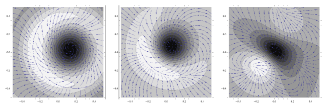
Figure 2: Examples of magnetogram sections are presented in the figure for C (left) and LL (center and right) modes. The parameters for the C modes are ($\alpha,n,m,r_{1},r_{2},\theta,\phi$)= (-10.95,2,10,1.35,1.85,0.3,-0.12) and the parameters for the LL modes are given by ($n,m,r_{1},\theta,\phi$)=(3,2,0.5,0.31,4.1) and (1.4,2,0.3,1.75,4.14) for the center and right panel respectively. The left and the center correspond to a double polarity region whereas the right panel represents a triple polarity region.

4 Summary & Conclusions

We have shown that there are two solutions possible (albeit known already and denoted here as C and LL) from the separability assumption. We calculate the energies and relative helicity of the allowed force free fields in a shell geometry. For the LL mode we were able to extend the solution set obtained in Low & Lou (1990) from $n=1$ to all rational values of $n=\displaystyle{\frac{p}{q}}$ by solving the eqn (5) for all cases of odd $p$ and for cases of $q>p$ for even $p$, in effect extending solution to practically all $n$. The results are presented in Table 1. The LL solution of ($n=1$ in Low & Lou (1990) and $n=5,7,9$ (odd cases) in Flyer et al. (2004)) have been extended here to the cases of nearly all $n$. The topological properties of these extended solutions can be further studied by considering other boundary conditions.The analytic solutions for LL suffer from the problem of a singularity at the origin which render them unphysical; this implies that more realistic boundary conditions are necessary. To learn more about the evolution and genesis of these structures, it would be useful to carry out dynamical simulations allowing for foot point motions with the analytic input fields constructed above to study how the non-linearity develops; a stability analysis of the non-linear modes would also useful tool (Berger (1985) has analyzed the linear constant $\alpha$ case). Clearly, these are difficult mathematical problems to be addressed in the future. We explore fits of these solutions to HINODE magnetograms of NOAA AR 10930, 10923 and 10933 and obtain the best fits to C and LL modes using the procedure discussed above in PMR14.

We would also like to thank Y. Yan and M. Wheatland for helpful discussions. AP would like to thank CSIR for the SPM fellowship.

References

- Amari et al. (2006) Amari, T., Boulmezaoud, T. Z., & Aly, J. J. 2006, A&A, 446, 691
- Berger (1985) Berger, M. A. 1985, ApJS, 59, 433
- Chandrasekhar (1956) Chandrasekhar, S. 1956, Proceedings of the National Academy of Science, 42, 1
- Finn & Antonsen (1983) Finn, J. M., & Antonsen, T. M., Jr. 1983, Physics of Fluids, 26, 3540
- Flyer et al. (2004) Flyer, N., Fornberg, B., Thomas, S., & Low, B. C. 2004, ApJ, 606, 1210
- Low & Lou (1990) Low, B. C., & Lou, Y. Q. 1990, ApJ, 352, 343
- Mangalam & Krishan (2000) Mangalam, A., & Krishan, V. 2000, Journal of Astrophysics and Astronomy, 21, 299
- McClymont et. al. (1997) McClymont, A. N., Jiao, L., & Mikić. 1997, Sol. Phys., 174, 191
- (9) Prasad A., Mangalam A. & Ravindra B., 2014, in press ApJ (PMR14)
- Wheatland et al. (2000) Wheatland, M. S., Sturrock, P. A., & Roumeliotis, G. 2000, ApJ, 540, 1150
- Wheatland & Leka (2010) Wheatland, M. S., & Leka, K. D., 2010, ApJ, 728, 112
- Wiegelmann (2004) Wiegelmann, T. 2004, Sol. Phys., 219, 87
- Yang et. al. (1986) Yang, W. H., Sturrock, P. A., & Antiochos, S. K. 1986, ApJ, 309, 383
- Yan & Sakurai (2000) Yan, Y. and Sakurai, T.: 2000, Sol. Phys., 195, 89.