General structure of quantum collisional models

Abstract

We point to the connection between a recently introduced class of non-Markovian master equations and the general structure of quantum collisional models. The basic construction relies on three basic ingredients: a collection of time dependent completely positive maps, a completely positive trace preserving transformation and a waiting time distribution characterizing a renewal process. The relationship between this construction and a Lindblad dynamics is clarified by expressing the solution of a Lindblad master equation in terms of demixtures over different stochastic trajectories for the statistical operator weighted by suitable probabilities on the trajectory space.

1 Introduction

The study of open quantum systems has a long history [1, 2], and an important and difficult topic from the very beginning was the treatment of non-Markovian dynamical evolutions. Such dynamics should describe memory effects, which typically appear in the presence of strong system environment interaction, at low temperature, or if the environment has a complex spectral density. Recently new important results have been obtained in the very definition of a non-Markovian dynamics [3, 4, 5], see e.g. [6] for a first summary of recent results.

A well know class of open system dynamics, which is considered to be Markovian whatever definition of non-Markovianity one adopts, even the more strict and close to the classical notion as discussed in [7, 8], is given by the generator of a completely positive quantum dynamical semigroup as obtained by Gorini, Kossakowski, Sudarshan and Lindblad [9, 10]. This result, besides providing a quite general class of well defined time evolutions for a system interacting with some environment, has many important special features [2, 11]. Among others, its operator structure can be naturally related to elementary physical interactions, and the solution of the master equation can be related to a measurement interpretation, arising as an average over suitable stochastic realizations depending on the measurement outcomes. A major effort in the description of open quantum systems is the quest for a generalization of this class of Markovian time evolutions, possibly keeping some of its nice features. The minimal requirement is the preservation of trace and positivity of the statistical operator, which is granted by complete positivity of the time evolution. However other interesting features in looking for extensions are given by a connection between the operator structure of the equation and physically relevant or addressable quantities, as well as a possible link to a realization of the overall dynamics in terms of simpler and experimentally more manageable evolutions. This is also one of the motivations behind the so called collisional models [12, 13, 14, 15], which describe the dynamics as the effect of repeated interactions with an environment, considered as isolated collisions.

2 Piecewise dynamics from Lindblad equation

In this paper we want to point out in which sense a recent result about a general class of non-Markovian time evolutions [16] can be seen as a generalization of the Lindblad master equation. That is to say in which sense it can be seen as a structure of master equation, whose solutions are warranted to provide a completely positive time evolution map, and which includes a semigroup evolution as a special case. We will see that it should more properly be seen as the general structure of a collisional model describable in terms of a closed evolution equation for the statistical operator of the system only. To this aim we consider a particular expression of the solution of the Lindblad dynamics, which opens the way for a general characterization of certain collisional models. Given an equation of the form

$$\frac{\mathrm{d}\rho}{{dt}} = \mathcal{L}\rho,$$ (1)

where $\rho$ denotes the statistical operator describing the open system and $\mathcal{L}$ is a linear superoperator, it has been shown that the ensuing dynamics is given by a semigroup of completely positive time evolutions if and only if the superoperator is of the form [9, 10]

$$\mathcal{L}\rho = \mathcal{L}_{R}\rho+\mathcal{J}\rho,$$

where

$$\mathcal{L}_{R}\rho = R\rho+\rho R^{{\dagger}}$$

$$R = -\frac{i}{\hbar}H-\frac{1}{2}\sum_{k}L_{k}^{{\dagger}}L_{k},$$

with $H$ a self-adjoint operator, and $\mathcal{J}$ denotes the completely positive superoperator

$$\mathcal{J}\rho = \sum_{k}L_{k}\rho L_{k}^{{\dagger}}.$$ (2)

Beside the completely positive map $\mathcal{J}$ it is natural to introduce the semigroup of completely positive trace decreasing superoperators $\mathcal{R}\left(t\right)$

$$\mathcal{R}\left(t\right)\rho = \mathrm{e}^{tR}\rho\mathrm{e}^{tR^{{\dagger}}}.$$ (3)

Together with the latter it is convenient for our purposes to introduce the following superoperators, which send positive operators to statistical operators

$$\mathcal{\tilde{J}}\sigma = \frac{\mathcal{J}\sigma}{{Tr}\left(\mathcal{J\sigma}\right)}$$ (4)

and

$$\tilde{\mathcal{R}}\left(t\right)\sigma = \frac{\mathcal{R}\left(t\right)\sigma}{{Tr}\left(\mathcal{R}\left(t\right)\sigma\right)}.$$ (5)

Note that the latter transformations, denoted by a tilda, are not linear, but rather homogeneous of order zero according to the relation

$$\mathcal{\widetilde{\mathcal{A}}}\left(\mu\sigma\right) = \mathcal{\tilde{A}}\sigma\hskip 20.00003pt\forall\mu\in\mathbbm{C}$$ (6)

which holds for both $\mathcal{\tilde{J}}$ and $\tilde{\mathcal{R}}\left(t\right)$, so that in particular if $\sigma$ is itself a statistical operator they can be seen as repreparations of the state according to the action of the map $\mathcal{J}$ or $\mathcal{R}\left(t\right)$ respectively. In terms of these operators the solution of Eq. (1) can be expressed as follows

$$\rho\left(t\right) = \pi^{0}_{t}\left(t\right)\tilde{\mathcal{R}}\left(t\right)\rho\left(0\right)+\sum_{n=1}^{\infty}\int^{t}_{0}\mathrm{d}t_{n}\ldots\int^{t_{2}}_{0}\mathrm{d}t_{1}\pi^{n}_{t}\left(t_{1},\ldots,t_{n}\right)$$

$$\hskip 20.00003pt\times\mathcal{\tilde{\mathcal{R}}}\left(t-t_{n}\right)\mathcal{\tilde{J}}\ldots\mathcal{\widetilde{J}}\mathcal{R}\left(t_{2}-t_{1}\right)\widetilde{\mathcal{J}}\mathcal{\widetilde{\mathcal{R}}}\left(t_{1}\right)\rho\left(0\right),$$

where besides the operators $\mathcal{\tilde{J}}$ and $\widetilde{\mathcal{R}}\left(t\right)$ defined in Eq. (4) and Eq. (5) respectively, we have defined the quantity

$$\pi^{0}_{t}\left(t\right) = {Tr}\left(\mathcal{R}\left(t\right)\rho\left(0\right)\right)$$ (8)

which can be interpreted as the probability of no jumps described by the superoperator $\mathcal{J}$ up to time $t$, while

$$\pi^{n}_{t}\left(t_{1},\ldots,t_{n}\right) = {Tr}\left(\mathcal{R}\left(t-t_{n}\right)\mathcal{J}\ldots\mathcal{J}\mathcal{R}\left(t_{2}-t_{1}\right)\mathcal{J}\mathcal{R}\left(t_{1}\right)\rho\left(0\right)\right),$$ (9)

can be taken as exclusive probability densities for the realization of $n$ jumps at the times $t_{1}<t_{2}<\ldots<t_{n-1}<t_{n}$ and no jumps in between up to time $t$ [17, 18]. This interpretation is justified by making reference to the use of stochastic master equations in the theory of continuous measurement [17, 19]. Note in particular the crucial fact that these probability densities do actually depend on the initial state, and not only on the operators appearing in the master equation. This interpretation as probability densities is most easily seen considering an interesting special case. Consider the situation in which the superoperator $\mathcal{\tilde{J}}$ sends each operator to a fixed statistical operator $\bar{\rho}$, so that

$$\mathcal{J}\sigma = \bar{\rho}{Tr}\left(\mathcal{J}\sigma\right).$$ (10)

In this case one has, starting from the state $\bar{\rho}$

$$\pi^{n}_{t}\left(t_{1},\ldots,t_{n}\right) = {Tr}\left(\mathcal{R}\left(t-t_{n}\right)\mathcal{J}\ldots\mathcal{J}\mathcal{R}\left(t_{2}-t_{1}\right)\mathcal{J}\mathcal{R}\left(t_{1}\right)\bar{\rho}\right)$$

$$= {Tr}\left(\mathcal{R}\left(t-t_{n}\right)\mathcal{J}\ldots\mathcal{J}\mathcal{R}\left(t_{2}-t_{1}\right)\bar{\rho}\right){Tr}\left(\mathcal{J}\mathcal{R}\left(t_{1}\right)\bar{\rho}\right)$$

$$= {Tr}\left(\mathcal{R}\left(t-t_{n}\right)\bar{\rho}\right)\ldots{Tr}\left(\mathcal{J}\mathcal{R}\left(t_{2}-t_{1}\right)\bar{\rho}\right){Tr}\left(\mathcal{J}\mathcal{R}\left(t_{1}\right)\bar{\rho}\right).$$

Setting

$$w_{0}\left(t\right) = {Tr}\left(\mathcal{}\mathcal{R}\left(t\right)\bar{\rho}\right)$$

$$w\left(t\right) = {Tr}\left(\mathcal{J}\mathcal{R}\left(t\right)\bar{\rho}\right),$$

thanks to the definition of the superoperators Eq. (2) and Eq. (3) one can immediately check the relation

$$\frac{\mathrm{d}w_{0}\left(t\right)}{{dt}} = -{Tr}\left(\mathcal{J}\mathcal{R}\left(t\right)\bar{\rho}\right)$$

$$= -w\left(t\right),$$

which given the fact that $w_{0}\left(t\right)$ has the properties of a survival probability, the probability of no jumps up to time $t$, implies that $w\left(t\right)$ is its associated waiting time distribution, the probability density for a count at time $t$, thus leading to the expression

$$\pi^{n}_{t}\left(t_{1},\ldots,t_{n}\right) = w_{0}\left(t-t_{n}\right)\ldots w\left(t_{2}-t_{1}\right)w\left(t_{1}\right),$$

which corresponds to a renewal process for the distribution in time of the jumps [20].

The expression of the solution of the master equation given by Eq. (2) can be seen as a demixture of the state at time $t$ in terms of states corresponding to possible trajectories. Each trajectory is specified by the number and the time of the counts or jumps. The states associated to the different trajectories are then weighted according to the probability densities on the trajectory space given by Eq. (9), which are determined by the quantum dynamics itself, and therefore provide the so called physical probabilities. The latter indeed allow to express the solution of the master equation as average over normalized states arising as solution of an associated nonlinear stochastic master equation and corresponding to different trajectories, see [17, 19] for a mathematically more precise treatment. Alternatively, always exploiting the formalism of stochastic master equations, one can express the solution of the master equation Eq. (1) by using as weight an arbitrary reference probability, independent from the initial state, e.g. a Poisson distribution with a fixed parameter $\lambda$, so that in this case the probability to have $n$ counts up to time $t$ at fixed times $t_{1}<t_{2}<\ldots<t_{n-1}<t_{n}$ is independent of the actual times $\left\{t_{i}\right\}_{i=1,\ldots,n}$ and is given by $\lambda^{n}\exp\left(-\lambda t\right)$. In this case however the state is expressed as demixture with these weights of unnormalized statistical operators $\tilde{\rho}\left(t\right)$, also called statistical subcollections, that is positive operators with trace less or equal than one, which arise as solution of a linear stochastic master equation and take the form [17, 19]

$$\tilde{\rho}\left(t\right) = \lambda^{-n}\exp\left(\lambda t\right)\mathcal{R}\left(t-t_{n}\right)\mathcal{J}\ldots\mathcal{J}\mathcal{R}\left(t_{2}-t_{1}\right)\mathcal{J}\mathcal{R}\left(t_{1}\right)\rho\left(0\right),$$ (12)

leading in the end to the standard expansion of the solution. Knowledge of the existence of the two alternatives will clarify the nature of the non-Markovian extension that we shall consider below, which can be seen as arising by merging the two viewpoints.

Before proceeding let us briefly show how to obtain Eq. (2) without the need to resort to the formalism of stochastic master equations for the statistical operator. Let us start from the expression of the solution in the familiar form of a Dyson series [21]

$$\rho\left(t\right) = \mathcal{R}\left(t\right)\rho\left(0\right)+\sum_{n=1}^{\infty}\int^{t}_{0}\mathrm{d}t_{n}\ldots\int^{t_{2}}_{0}\mathrm{d}t_{1}$$

$$\hskip 20.00003pt\times\mathcal{R}\left(t-t_{n}\right)\mathcal{J}\ldots\mathcal{J}\mathcal{R}\left(t_{2}-t_{1}\right)\mathcal{J}\mathcal{R}\left(t_{1}\right)\rho\left(0\right),$$

which in particular at variance with Eq. (2) immediately shows linearity and complete positivity of the time evolution. Note further that according to the given definitions Eq. (5) and Eq. (8) one immediately has the relation

$$\mathcal{R}\left(t\right)\sigma = {Tr}\left(\mathcal{R}\left(t\right)\sigma\right)\frac{\mathcal{R}\left(t\right)\sigma}{{Tr}\left(\mathcal{R}\left(t\right)\sigma\right)}$$

$$= \pi^{0}_{t}\left(t\right)\tilde{\mathcal{R}}\left(t\right)\sigma.$$

Moreover for any superoperator $\mathcal{\tilde{A}}$ homogeneous of order zero according to Eq. (6) one can immediately verify the relation

$$\mathcal{\tilde{A}}\mathcal{R}\left(t-t_{n}\right)\mathcal{J}\ldots\mathcal{J}\mathcal{R}\left(t_{1}\right) = \mathcal{\tilde{A}}\mathcal{}\mathcal{\tilde{\mathcal{R}}}\left(t-t_{n}\right)\mathcal{\tilde{J}}\ldots\mathcal{\tilde{J}}\mathcal{\widetilde{\mathcal{R}}}\left(t_{1}\right),$$

so that one has the simple basic relationship

$$\mathcal{R}\left(t-t_{n}\right)\mathcal{J}\ldots\mathcal{J}\mathcal{R}\left(t_{1}\right)\rho\left(0\right) = {Tr}\left(\mathcal{R}\left(t-t_{n}\right)\mathcal{J}\ldots\mathcal{J}\mathcal{R}\left(t_{1}\right)\rho\left(0\right)\right)$$

$$\hskip 10.00002pt\times\frac{\mathcal{R}\left(t-t_{n}\right)\mathcal{J}\ldots\mathcal{J}\mathcal{R}\left(t_{1}\right)\rho\left(0\right)}{{Tr}\left(\mathcal{R}\left(t-t_{n}\right)\mathcal{J}\ldots\mathcal{J}\mathcal{R}\left(t_{1}\right)\rho\left(0\right)\right)}$$

$$= \pi^{n}_{t}\left(t_{1},\ldots,t_{n}\right)\mathcal{\tilde{\mathcal{R}}}\left(t-t_{n}\right)\mathcal{\tilde{J}}\ldots\mathcal{\tilde{J}}\mathcal{\widetilde{\mathcal{R}}}\left(t_{1}\right),$$

which proves Eq. (2). Note that in general the probability densities $\pi^{n}_{t}\left(t_{1},\ldots,t_{n}\right)$ do not have any special properties, apart from being positive and normalized to one when summed over all $n$ and integrated over all possible intermediate times. As discussed above a simple situation only appears if the jump operator sends a generic state to a fixed operator. In this case the probability densities can be expressed in terms of a unique waiting time distribution.

3 Collisional models from piecewise dynamics

In the previous Section we have provided through Eq. (2) a particular representation of the statistical operator solution of a Lindblad dynamics, which is alternative to the usual Dyson expansion of the solution, corresponding to Eq. (2). Eq. (2) is the most natural starting point to come to a general expression for a collisional dynamical model. Indeed in a collisional model a dynamics is obtained for a reduced system by building on three basic quantities. An intercollision time evolution, which describes the dynamics of the reduced system in between certain interaction events that can be considered localized in time, a state transformation described by a quantum channel which describes jumps or events, the correlation in time between these jumps, which can be described in terms of the probability density for the jump distribution. Expression Eq. (2) is suggestive in this respect, since all three elements appear in it. However there is a basic difference in that the dynamics in between jumps and the effect of the events described as collisions is not described by linear operators, but rather by the state transformations Eq. (3) and Eq. (2) respectively. We will however take this starting point to justify the class of non-Markovian dynamics obtained in [16], better elucidating its relationship with the Lindblad result. This will partially overcome the sudden leap made in [16] from the Dyson expansion to the generalized master equation, and explain why the standard Lindblad result is actually only obtained in a trivial limit.

In Eq. (2) the weight of the trajectories, expressed by the so called physical probability densities, are determined by the operators describing the dynamics, and the two objects are actually intertwined, as appears from the fact that in the alternative expression Eq. (2), as well as in the mixture in terms of unnormalized statistical operators given by Eq. (12), the physical probability densities do not directly appear. The idea is now to make the probability densities which give the weight of the trajectories independent from the state transformations between jumps, as well as from the explicit expression of the jumps operator, thus introducing an external non trivial distribution of jumps. This is one of the ingredients in a collisional model. At the same time in order to preserve linearity and granting complete positivity, we replace the non linear operators $\mathcal{\tilde{J}}$ and $\mathcal{\tilde{\mathcal{R}}}\left(t\right)$, with linear completely positive trace preserving transformations, which provide the other two ingredients of collisional models. Let us therefore consider the expression

$$\rho\left(t\right) = p_{0}\left(t\right)\mathcal{F}\left(t\right)\rho\!\left(0\right)+\!\sum_{n=1}^{\infty}\int^{t}_{0}\mathrm{d}t_{n}\ldots\int^{t_{2}}_{0}\mathrm{d}t_{1}$$

$$\hskip 20.00003pt\times p_{n}\left(t_{n},\ldots,t_{1}\right)\mathcal{F}\left(t-t_{n}\right)\mathcal{E}\ldots\mathcal{E}\mathcal{F}\left(t_{2}-t_{1}\right)\mathcal{E}\mathcal{F}\left(t_{1}\right)\rho\left(0\right)$$

where $p_{n}\left(t_{n},\ldots_{,}t_{1}\right)$ denotes the probability density for the realization of $n$ events up to time $t$, while $\mathcal{E}$ and $\mathcal{F}\left(t\right)$ denote respectively a completely positive trace preserving superoperator and a collection of completely positive time dependent evolutions. Such an expression provides by construction a realization of a collisional model and realizes a completely positive transformation on the space of statistical operators. In the general case however, for a generic weight associated to the different trajectories, that is a generic distribution of the interaction events, it is not possible to provide closed evolution equations for the statistical operator of the reduced system only. This is however the case for a distribution of jumps described by a renewal process, so that the probability densities read

$$p_{n}\left(t_{n},\ldots_{,}t_{1}\right) = f\left(t-t_{n}\right)\ldots f\left(t_{2}-t_{1}\right)g\left(t_{1}\right),$$ (15)

with $f\left(t\right)$ a waiting time distribution, that is a probability density over the positive reals and $g\left(t\right)$ its associated survival probability according to the relation

$$g\left(t\right) = 1-\int^{t}_{0}\mathrm{d}\tau f\left(\tau\right).$$

These relations lead to the expression

$$\rho\left(t\right) = p_{0}\left(t\right)\mathcal{F}\left(t\right)\rho\!\left(0\right)+\!\sum_{n=1}^{\infty}\int^{t}_{0}\mathrm{d}t_{n}\ldots\int^{t_{2}}_{0}\mathrm{d}t_{1}$$

$$\hskip 20.00003pt\times f\left(t-t_{n}\right)\mathcal{F}\left(t-t_{n}\right)\mathcal{E}\ldots\mathcal{E}f\left(t_{2}-t_{1}\right)\mathcal{F}\left(t_{2}-t_{1}\right)\mathcal{E}g\left(t_{1}\right)\mathcal{F}\left(t_{1}\right)\rho\left(0\right),$$

schematically depicted in Fig. 1

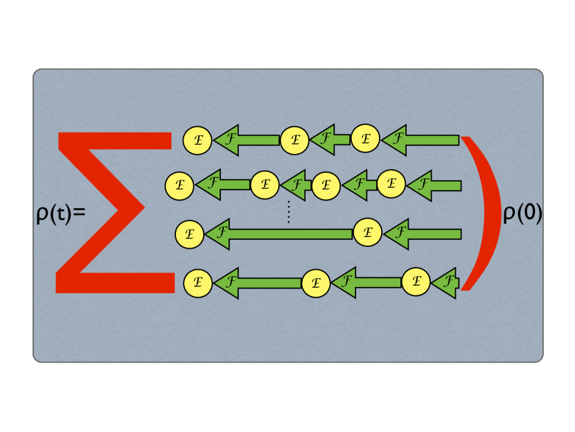
Figure 1: Pictorial representation of the dynamics arising from Eq. (3) according to its trajectory representation as given by Eq. (3). The statistical operator at time $t$ arises by summing over all trajectories characterized by the repeated action of the completely positive trace preserving map $\mathcal{E}$ at jump times determined by a fixed waiting time distribution, corresponding to the same type of arrows, while the different length of the arrows represents the time in between jumps. During this time the system is acted upon by a fixed time dependent dynamical map given by $\mathcal{F}$.

, where a pictorial scheme of the corresponding dynamics is given. From Eq. (3) one obtains the integral equation

$$\rho\left(t\right) = g\left(t\right)\mathcal{F}\left(t\right)\!+\!\int^{t}_{0}\mathrm{d}\tau f\left(t-\tau\right)\mathcal{F}\left(t-\tau\right)\mathcal{E}\rho\left(\tau\right),$$ (17)

which using the notation $\hat{h}\left(u\right)=\int^{\infty}_{0}\mathrm{d}t\mathrm{e}^{-ut}h\left(t\right)$ for the Laplace transform, reads

$$\hat{\rho}\left(u\right) = \widehat{g\mathcal{F}}\left(u\right)+\widehat{f\mathcal{F}}\left(u\right)\mathcal{E}\hat{\rho}\left(u\right).$$ (18)

This expression leads to a formally exact expression for the solution in the form

$$\hat{\rho}\left(u\right) = \left[\mathbbm{1}-\widehat{f\mathcal{F}}\left(u\right)\mathcal{E}\right]^{-1}\widehat{g\mathcal{F}}\left(u\right).$$ (19)

Moreover if we start from Eq. (18), with simple algebra, exploiting the initial conditions $g\left(0\right)=1$ and $\mathcal{F}\left(0\right)=\mathbbm{1}$, one comes to

$$u\hat{\rho}\left(u\right)-\mathbbm{1} = \left[u\widehat{g\mathcal{F}}\left(u\right)-\mathbbm{1}\right]+\left[u\widehat{f\mathcal{F}}\left(u\right)-f\left(0\right)\right]\mathcal{E}\hat{\rho}\left(u\right)+f\left(0\right)\mathcal{E}\hat{\rho}\left(u\right),$$

leading by inversion of the Laplace transform to the closed integrodifferential equation obeyed by the statistical operator of the reduced system

$$\frac{\mathrm{d}}{\mathrm{d}t}\rho\left(t\right) = \int^{t}_{0}\mathrm{d}\tau\frac{\mathrm{d}}{\mathrm{d}\left(t-\tau\right)}f\left(t-\tau\right)\mathcal{F}\left(t-\tau\right)\mathcal{E}\rho\left(\tau\right)$$

$$+f\left(0\right)\mathcal{E}\rho\left(t\right)+\frac{\mathrm{d}}{\mathrm{d}t}\left[g\left(t\right)\mathcal{F}\left(t\right)\right].$$

As we have shown this result arises building on the representation of the Lindblad dynamics as given by Eq. (2), by substituting the physical probabilities with a set of probability densities determined by a single waiting time distribution $f\left(t\right)$ which can be arbitrarily fixed, and replacing the non linear transformations $\mathcal{\tilde{J}}$ and $\mathcal{\tilde{\mathcal{R}}}\left(t\right)$, describing a measurement transformation of the state and strictly connected through Eq. (2) and Eq. (3), with the linear completely positive trace preserving maps $\mathcal{E}$ and $\mathcal{F}\left(t\right)$ which can be taken independent of each other. Indeed this changes deeply modify the Lindblad dynamics, replacing it with a piecewise dynamics characterized by three independent quantities, so that the distribution of the jumps is not dictated anymore by the dynamics itself as in Eq. (9) and conditioned by the initial state, but rather given by an external counter. This is reflected by the fact that the Lindblad dynamics is only recovered in the trivial limit $\mathcal{F}\left(t\right)\rightarrow\mathrm{e}^{t\mathcal{L}}$, with $\mathcal{L}$ a superoperator in Lindblad form and $\mathcal{E}\rightarrow\mathbbm{1}$, independently of the chosen waiting time distribution. The most natural interpretation of Eq. (3) is therefore as a general scheme of collisional model.

Two important questions related to the obtained completely positive piecewise dynamics are its degree of non-Markovianity and the possibility to obtain it as a reduced dynamics from an overall Markovian dynamics in a larger space. The possible degree of non-Markovianity of these time evolutions has been discussed in [16], together with the connection with different master equations related to collisional models, relying on a recently introduced notion of non-Markovianity based on the behavior in time of the distinguishability of different initial reduced states [3, 22]. The embedding of these dynamics into a Markovian dynamics in a larger Hilbert space has been most recently addressed in [18, 23].

4 Conclusions and outlook

We have addressed how to formulate a Lindblad dynamics so as to open the way for the introduction of a general structure of time evolution described by a collisional model, which allows to consider general non-Markovian dynamics. This has been obtained by expressing the time evolved statistical operator as an average over trajectories, weighted by physical probabilities which are determined by the operators appearing in the Lindblad master equation, intertwined among them due to probability conservation. Suitably considering these three elements as independent allows to describe a more general yet closed piecewise dynamics. This result has opened the way to the study of the degree of non-Markovianity of the ensuing dynamics, and to the exploration of their embedding in a Markovian framework in a larger space. It further calls for microscopic derivations, which could shed light on physically motivated choices of the waiting time distribution and of the otherwise arbitrary completely positive trace preserving maps realizing the evolution.

Acknowledgments.

The author thanks Prof. Alberto Barchielli for many useful discussions. Support from COST Action MP 1006 is gratefully acknowledged.

References

- [1] E. B. Davies, Quantum Theory of Open Systems (Academic Press, London, 1976)
- [2] H.-P. Breuer and F. Petruccione, The Theory of Open Quantum Systems (Oxford University Press, Oxford, 2007)
- [3] H.-P. Breuer, E.-M. Laine, and J. Piilo, Phys. Rev. Lett. 103, 210401 (2009)
- [4] A. Rivas, S. F. Huelga, and M. B. Plenio, Phys. Rev. Lett. 105, 050403 (2010)
- [5] M. M. Wolf, J. Eisert, T. S. Cubitt, and J. I. Cirac, Phys. Rev. Lett. 101, 150402 (2008)
- [6] H.-P. Breuer, J. Phys. B 45, 154001 (2012)
- [7] G. Lindblad, Comm. Math. Phys. 65, 281 (1979)
- [8] R. Dümcke, J. Math. Phys. 24, 311 (1983)
- [9] V. Gorini, A. Kossakowski, and E. C. G. Sudarshan, J. Math. Phys. 17, 821 (1976)
- [10] G. Lindblad, Comm. Math. Phys. 48, 119 (1976)
- [11] A. Rivas and S. F. Huelga, Open Quantum Systems: An Introduction (Springer, 2012)
- [12] M. Ziman, P. Štelmachovič, and V. Bužek, Open Syst. Inf. Dyn. 12, 81 (2005)
- [13] T. Rybár, S. N. Filippov, M. Ziman, and V. Bužek, J. Phys. B 45, 154006 (2012)
- [14] V. Giovannetti and G. M. Palma, J. Phys. B 45, 154003 (2012)
- [15] F. Ciccarello, G. M. Palma, and V. Giovannetti, Phys. Rev. A 87(040103(R)) (2013)
- [16] B. Vacchini, Phys. Rev. A 87, 030101(R) (2013)
- [17] A. Barchielli, Some stochastic di erential equations in quantum optics and measurement theory: the case of counting processes., in Stochastic Evolution of Quantum States in Open Systems and in Measurement Processes, edited by L. Diósi and B. Lukàcs (World Scientific, Singapore, 1994), pp. 1–14
- [18] A. A. Budini, Phys. Rev. A 88, 032115 (2013)
- [19] A. Barchielli and M. Gregoratti, Quantum Trajectories and Measurements in Continuous Time, Vol. 782 of Lecture Notes in Physics (Springer, Berlin, 2009)
- [20] S. M. Ross, Introduction to probability models (Academic Press, Burlington, MA, 2007)
- [21] A. S. Holevo, Statistical Structure of Quantum Theory, Vol. m 67 of Lecture Notes in Physics (Springer, Berlin, 2001)
- [22] E.-M. Laine, J. Piilo, and H.-P. Breuer, Phys. Rev. A 81, 062115 (2010)
- [23] A. A. Budini, Phys. Rev. A 88, 012124 (2013)