On the low lying spectrum of the magnetic Schrödinger operator with kagome periodicity

Abstract

We study in a semi-classical regime a periodic magnetic Schrödinger operator in $\mathbb{R}^{2}$. This is inspired by recent experiments on artificial magnetism with ultra cold atoms in optical lattices, and by the new interest for the operator on the hexagonal lattice describing the behavior of an electron in a graphene sheet. We first review some results for the square (Harper), triangular and hexagonal lattices. Then we study the case when the periodicity is given by the kagome lattice considered by Hou. Following the techniques introduced by Helffer-Sjöstrand and Carlsson, we reduce this problem to the study of a discrete operator on $\ell^{2}(\mathbb{Z}^{2};\mathbb{C}^{3})$ and a pseudo-differential operator on $L^{2}(\mathbb{R};\mathbb{C}^{3})$, which keep the symmetries of the kagome lattice. We estimate the coefficients of these operators in the case of a weak constant magnetic field. Plotting the spectrum for rational values of the magnetic flux divided by $2\pi h$ where $h$ is the semi-classical parameter, we obtain a picture similar to Hofstadter’s butterfly. We study the properties of this picture and prove the symmetries of the spectrum and the existence of flat bands, which do not occur in the case of the three previous models.

1 Introduction

We consider in a semi-classical regime the Schrödinger magnetic operator $P_{h,A,V}$, defined as the self-adjoint extension in $L^{2}(\mathbb{R}^{2})$ of the operator given in $C_{0}^{\infty}(\mathbb{R}^{2})$ by

$$P_{h,A,V}^{0}=(hD_{x_{1}}-A_{1}(x))^{2}+(hD_{x_{2}}-A_{2}(x))^{2}+V(x)\,,$$ (1.1)

where $D_{x_{j}}=\frac{1}{i}\partial_{x_{j}}$. Our goal is to study the spectrum of $P_{h,A,V}$ as a function of $A$ and the semi-classical parameter $h>0$, when $V$ has its minima in the kagome lattice and both $V$ and $B=\nabla\wedge A$ are invariant by the symmetries of the kagome lattice.

Our interest in this mathematical problem is motivated by recent experiments on artificial magnetism with ultra cold atoms ([DGJO11, JZ03]), that lead to new geometries for this problem. To our knowledge, the Hamiltonian in (1.1) has not been obtained in a laboratory with ultra cold atoms, but we mention that a two-dimensional kagome lattice for ultra cold atoms has been recently achieved ([JGT⁺12]) using optical potentials. Our main motivation is to understand and analyze mathematically various considerations of Hou in [Hou09].

Let us explain the setting of our problem. A n-dimensional Bravais lattice is the set of points spanned over $\mathbb{Z}$ by the vectors of a basis $\{\nu_{1},\cdots,\nu_{n}\}$ of $\mathbb{R}^{n}$. A fundamental domain of the Bravais lattice is a domain of the form

$$\mathcal{V}=\big{\{}t_{1}\nu_{1}+\cdots+t_{n}\nu_{n}\,;\,t_{1},\cdots,t_{n}\in[0,1]\big{\}}\,.$$

The kagome lattice is not a Bravais lattice, but is a discrete subset of $\mathbb{R}^{2}$ invariant under translations along a triangular lattice and containing three points per fundamental domain of this lattice (see Figures 1 and 6d). Each point of the lattice has four nearest neighbours for the Euclidean distance. The word kagome means a bamboo-basket (kago) woven pattern (me) and it seems that the lattice was named by the Japanese physicist K. Husimi in the 50’s ([Mek03]).

Let $\Gamma_{\triangle}$ be the triangular lattice spanned by $\mathcal{B}=\{2\nu_{1},2\nu_{2}\}$, where

$$\nu_{\ell}=r^{\ell-1}(1,0)$$ (1.2)

and $r$ is the rotation of angle $\nicefrac{{\pi}}{{3}}$ and center the origin. The kagome lattice can be seen as the union of three conveniently translated copies of $\Gamma_{\triangle}$ :

$$\Gamma=\Big{\{}m_{\alpha,\ell}=2\alpha_{1}\nu_{1}+2\alpha_{2}\nu_{2}+\nu_{\ell}\,;\,(\alpha_{1},\alpha_{2})\in\mathbb{Z}^{2}\,,\,\ell=1,3,5\Big{\}}\,.$$ (1.3)

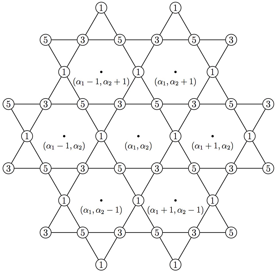
Figure 1: The kagome lattice and its labelling.

We label the points of $\Gamma$ by their coordinates in $\mathcal{B}$:

$$\tilde{\Gamma}=\Big{\{}\tilde{m}_{\alpha,\ell}=(\alpha_{1},\alpha_{2})+\tilde{\nu}_{\ell}\,;\,(\alpha_{1},\alpha_{2})\in\mathbb{Z}^{2}\,,\,\ell=1,3,5\Big{\}}\,,$$

where

$$\tilde{\nu}_{\ell}=\frac{1}{2}\kappa^{\ell-1}(1,0)$$ (1.4)

are the coordinates of $\nu_{j}$ in the basis $\mathcal{B}$. The map $\kappa:\mathbb{Z}^{2}\to\mathbb{Z}^{2}$ here before is given by

$$\kappa(\alpha_{1},\alpha_{2})=(-\alpha_{2},\alpha_{1}+\alpha_{2})$$ (1.5)

and represents the rotation $r$ in the basis $\mathcal{B}$, that is, $\widetilde{r(m_{\alpha,\ell})}=\kappa(\tilde{m}_{\alpha,\ell})$.

We will often consider $j=1,\dots,6$ as an element of $\nicefrac{{\mathbb{Z}}}{{6\mathbb{Z}}}$. Depending on the situation, we will give the properties of the kagome lattice in terms of the points $m_{\alpha,\ell}$ or in terms of their coordinates $\tilde{m}_{\alpha,\ell}$.

The symmetries of $\Gamma$ are given by those of $\Gamma_{\triangle}$. For $j\in\nicefrac{{\mathbb{Z}}}{{6\mathbb{Z}}}$ consider the translations $t_{j}(x)=x+2\nu_{j}$ and define

$$\mathcal{G}=\text{the subgroup of the affine group of the plane generated by }r,\,t_{1}\text{ and }t_{2}\,.$$ (1.6)

Setting $(gu)(x)=u(g^{-1}(x))$ for $g\in\mathcal{G}$, we define a group action of $\mathcal{G}$ on $C^{\infty}(\mathbb{R}^{2})$ which can be extended as an unitary action on $L^{2}(\mathbb{R}^{2})$.

Hypothesis 1.1.

The electric potential $V$ is a real nonnegative $C^{\infty}$ function such that

$$gV=V\quad\text{ for all }g\in\mathcal{G}\,,$$ (1.7)

$$V\geq 0\quad\text{ and }\quad V(x)=0\text{ if and only if }x\in\Gamma\,,$$ (1.8)

$${\rm Hess}\,V(x)>0\quad\forall x\in\Gamma\,.$$ (1.9)

We associated with the magnetic vector potential $A=(A_{1},A_{2})$ the 1-form

$$\omega_{A}=A_{1}dx_{1}+A_{2}dx_{2}\,.$$

The magnetic field $B$ is then associated with the 2-form obtained by taking the exterior derivative of $\omega_{A}$:

$$d\omega_{A}=B(x)dx_{1}\wedge dx_{2}\,.$$

In the case of $\mathbb{R}^{2}$, we identify this 2-form with $B$. The renormalized flux of $B$ through a fundamental domain $\mathcal{V}$ of $\Gamma_{\triangle}$ is by definition

$$\gamma=\frac{1}{h}\int_{\mathcal{V}}d\omega_{A}\,.$$

Hypothesis 1.2.

The magnetic potential $A$ is a $C^{\infty}$ vector field such that the corresponding magnetic 2 form satisfies

$$gB=B\quad\text{ for all }g\in\mathcal{G}\,.$$ (1.10)

In the case when $A=0$ (see for example Chapter XIII.16 in [RS80]), the spectrum of $P_{h,A,V}$ is continuous and composed of bands. The general case, even when the magnetic field is constant, is very delicate. The spectrum of $P_{h,A,V}$ can indeed become very singular (Cantor structure) and depends crucially on the arithmetic properties of $\gamma/(2\pi)$.

To approach this problem, we are often led to the study of limiting models in different asymptotic regimes, such as discrete operators defined over $\ell^{2}(\mathbb{Z}^{2};\mathbb{C}^{n})$, or equivalently, $\gamma$-pseudo-differential operators defined on $L^{2}(\mathbb{R};\mathbb{C}^{n})$ and associated with periodical symbols.

The discrete operators considered are polynomials in $\tau_{1}$, $\tau_{2}$, $\tau^{*}_{1}$ and $\tau_{2}^{*}$ with coefficients in $M_{n}(\mathbb{C})$, where $\tau_{1}$ and $\tau_{2}$ are the discrete magnetic translations on $\ell^{2}(\mathbb{Z}^{2};\mathbb{C}^{n})$ given by

$$(\tau_{1}v)_{\alpha}=v_{\alpha_{1}-1,\alpha_{2}}\,,\qquad(\tau_{2}v)_{\alpha}=e^{i\gamma\alpha_{1}}v_{\alpha_{1},\alpha_{2}-1}\,.$$ (1.11)

We also recall that the $\gamma$-quantization of a symbol $p(x,\xi,\gamma)$ with values in $M_{n}(\mathbb{C})$ is the pseudo-differential operator defined over $L^{2}(\mathbb{R};\mathbb{C}^{n})$ by

$$\left((\text{Op}_{\gamma}^{W}p)u\right)(x)=\frac{1}{{2\pi}\gamma}\int\!\!\!\int_{\mathbb{R}^{2}}e^{i\frac{(x-y)\xi}{\gamma}}p\left(\frac{x+y}{2},\xi,\gamma\right)\,u(y)\,dy\,d\xi\,.$$ (1.12)

In this article, following the ideas in [HS88a], §9, we first analyze the restriction of $P_{h,A,V}$ to a spectral space associated with the bottom of its spectrum, and we show the existence of a basis of this space such that the matrix of this operator keeps the symmetries of $\Gamma$.

In order to state our first theorem, let us explain more in detail this procedure. First of all, the harmonic approximation together with Agmon estimates shows the existence of an exponentially small (with respect to $h$) band in which one part of the spectrum (including the bottom) of $P_{h,A,V}$ is confined. We name this part the low lying spectrum. The rest of the spectrum is separated by a gap of size $h/C$.

Consider $\delta\in(0,1/8)$ and a non negative radial smooth function $\chi$, such that $\chi=1$ in $B(0,\delta/2)$ and $\text{supp}\,\chi\subset B(0,\delta)$. For any $m\in\Gamma$ define

$$V_{m}(\cdot)=\sum_{n\in\Gamma\setminus\{m\}}\chi(\cdot-n)$$

and

$$P_{m}=P_{h,A,V}+V_{m}\,.$$ (1.13)

All the $P_{m}$ are unitary equivalent and

$$b=\liminf_{|x|\to\infty}V_{m}(x)$$ (1.14)

is positive and does not depend on $m$. The spectrum of $P_{m}$ is discrete in the interval $[0,b]$. The first eigenvalue of $P_{m}$ is simple and we note it $\lambda(h)$. We can prove that there exists then $\epsilon_{0}>0$ such that $\sigma(P_{m})\cap I(h)=\{\lambda(h)\}$, where $I(h)=[0,h(\lambda_{har,1}+\epsilon_{0})]$ and $\lambda_{har,1}$ is the first eigenvalue of the operator associated with $P_{m}$ by the harmonic approximation when $h=1$ (see Section 5.3 for more details). We define

$$\Sigma=\text{ the spectral space associated with }I(h)\,.$$ (1.15)

We denote by $d_{V}$ the Agmon distance associated with the metric $Vdx^{2}$ (see [DS99], §6) and

$$S=\min\{d_{V}(n,m);\,n,m\in\Gamma,\,n\not=m\}.$$ (1.16)

We then have:

Theorem 1.3.

Under Hypotheses 1.1 and 1.2, there exists $h_{0}>0$ such that for $h\in(0,h_{0})$ there exists a basis of $\Sigma$ in which $P_{h,A,V}\big{|}\Sigma$ has the matrix

$$\lambda(h)I+W_{\gamma}\,,$$

where for all $\tilde{n},\tilde{m}\in\tilde{\Gamma}$ and $\alpha\in\mathbb{Z}^{2}$, $W_{\gamma}$ satisfies

$$(W_{\gamma})_{\tilde{n},\tilde{m}} = \overline{(W_{\gamma})_{\tilde{m},\tilde{n}}}\,,$$ (1.17)

$$(W_{\gamma})_{\tilde{n},\tilde{m}} = e^{-i\frac{\gamma}{2}(\tilde{m}-\tilde{n})\wedge\alpha}(W_{\gamma})_{(\tilde{n}+\alpha),(\tilde{m}+\alpha)}\,,$$ (1.18)

$$(W_{\gamma})_{\tilde{n},\tilde{m}} = (W_{\gamma})_{\kappa(\tilde{n}),\kappa(\tilde{m})}\,.$$ (1.19)

Moreover, there exists $C>0$ such that for every $\epsilon>0$ there exists $h_{\epsilon}>0$, such that for $h\in(0,h_{\epsilon})$

$$|(W_{\gamma})_{\tilde{n},\tilde{m}}| \leq C\,\exp\left(-\frac{(1-\epsilon)d_{V}(m,n)}{h}\right)\,,$$ (1.20)

$$|(W_{\gamma})_{\tilde{n},\tilde{n}}| \leq C\,\exp\left(-\frac{(2S-\epsilon)}{h}\right)\,.$$ (1.21)

The coefficients of $W_{\gamma}$ are related to the interaction between different sites of the kagome lattice. Our next result concerns the study of this matrix, when we only keep the main terms for the Agmon distance. In order to estimate these terms, we need additional hypothesis. Here we assume (see [HS84] for more details):

Hypothesis 1.4.

• The nearest neighbors for the Agmon distance are the same of those for the Euclidean distance, i.e.  $S=d_{V}\left(m_{(1,0),3},m_{(0,0),1}\right)$.

• Between two nearest neighbors $m,n\in\Gamma$ there exists an unique minimal geodesic $\zeta_{m,n}$ for the Agmon metric.

• This geodesic $\zeta_{m,n}$ coincides with the Euclidean one that is the segment between $m$ and $n$.

• The geodesic $\zeta_{m,n}$ in non degenerate in the sense that there is a point $x_{0}\in\zeta_{m,n}\setminus\{m,n\}$ such that the function $x\mapsto d_{V}(x,m)+d_{V}(x,n)-d_{V}(m,n)$ restricted to a transverse line to $\zeta_{m,n}$ at $x_{0}$ has a non degenerate local minimum at $x_{0}$.

Under this hypothesis, we will estimate the main terms in the case of a weak and constant magnetic field $B=hB_{0}$, given by the gauge

$$A(x_{1},x_{2})=\frac{hB_{0}}{2}(-x_{2},x_{1})\,,\quad B_{0}>0\,.$$ (1.22)

The discrete model associated with the kagome lattice is

$$Q_{\gamma,\omega}=\left(\begin{array}[]{ccc}0&e^{i(\omega+\frac{\gamma}{8})}\left(\tau_{1}^{*}+e^{-i\frac{\gamma}{2}}\tau_{1}^{*}\tau_{2}\right)&e^{-i(\omega+\frac{\gamma}{8})}\left(\tau_{1}^{*}+\tau_{2}^{*}\right)\\ e^{-i(\omega+\frac{\gamma}{8})}\left(\tau_{1}+e^{-i\frac{\gamma}{2}}\tau_{1}\tau_{2}^{*}\right)&0&e^{i(\omega+\frac{\gamma}{8})}\left(e^{-i\frac{\gamma}{2}}\tau_{1}\tau_{2}^{*}+\tau_{2}^{*}\right)\\ e^{i(\omega+\frac{\gamma}{8})}\left(\tau_{1}+\tau_{2}\right)&e^{-i(\omega+\frac{\gamma}{8})}\left(e^{-i\frac{\gamma}{2}}\tau_{1}^{*}\tau_{2}+\tau_{2}\right)&0\end{array}\right)$$ (1.23)

acting on $\ell^{2}(\mathbb{Z}^{2};\,\mathbb{C}^{3})$.

We also introduce the symbol

$$p^{kag}(x,\xi,\gamma,\omega)=\left(\begin{array}[]{ccc}0&e^{i(\omega+\frac{\gamma}{8})}\left(e^{-ix}+e^{-i(x-\xi)}\right)&e^{-i(\omega+\frac{\gamma}{8})}\left(e^{-ix}+e^{-i\xi}\right)\\ e^{-i(\omega+i\frac{\gamma}{8})}\left(e^{ix}+e^{i(x-\xi)}\right)&0&e^{i(\omega+\frac{\gamma}{8})}\left(e^{i(x-\xi)}+e^{-i\xi}\right)\\ e^{i(\omega+\frac{\gamma}{8})}\left(e^{ix}+e^{i\xi}\right)&e^{-i(\omega+\frac{\gamma}{8})}\left(e^{-i(x-\xi)}+e^{i\xi}\right)&0\end{array}\right)$$ (1.24)

and its Weyl-quantization $P^{kag}_{\gamma,\omega}={\rm Op}^{W}_{\gamma}p^{kag}(x,\xi,\gamma,\omega)$ acting on $L^{2}(\mathbb{R};\,\mathbb{C}^{3})$.

We now state two theorems linking the Schrödinger operator and these two models.

Theorem 1.5.

Let $V$ satisfies Hypothesis 1.4. There exists $b_{0}>0$, $h_{0}>0$, $C>0$ and $R\in\mathcal{L}(\ell^{2}(\mathbb{Z}^{2};\,\mathbb{C}^{3}))$ such that for $h\in(0,h_{0})$, $P_{h,A,V}|\Sigma$ is unitary equivalent with

$$Q_{\gamma}=\lambda(h)\,I-\rho\left(Q_{\gamma,\omega}+R_{\gamma}\right)\,,$$ (1.25)

where

$$\rho = h^{\nicefrac{{1}}{{2}}}\,b_{0}\,e^{-\frac{S}{h}}\left(1+\mathcal{O}(h)\right)\,,$$ (1.26)

$$\omega = \mathcal{O}(h)$$ (1.27)

and

$$\|R_{\gamma}\|_{\mathcal{L}(\ell^{2}(\mathbb{Z}^{2};\mathbb{C}^{3}))}\leq C\,\exp\left(-\frac{1}{Ch}\right)\,.$$ (1.28)

Theorem 1.6.

Under the same Hypothesis of Theorem 1.5, there exists a symbol $r(x,\xi)$ $2\pi$-periodic in $x$ and $\xi$ such that $P_{h,A,V}|\Sigma$ has the same spectrum than

$$\lambda(h)\,I-\rho\left(P^{kag}_{\gamma,\omega}+{\rm Op}^{W}_{\gamma}r(x,\xi)\right)\,,$$ (1.29)

where $\rho$ and $\omega$ are given by (1.26) and (1.27), and

$$\|{\rm Op}^{W}_{\gamma}r(x,\xi)\|_{\mathcal{L}(L^{2}(\mathbb{R};\,\mathbb{C}^{3}))}\leq C\,\exp\left(-\frac{1}{Ch}\right)\,.$$ (1.30)

Remark 1.7.

In the case of the square, triangular and hexagonal lattices, using Hypothesis 1.1 and 1.2, it is possible to prove that the terms corresponding to the interaction between nearest neighbours of the lattices are equal, so $\omega=0$. The situation is more complex for the kagome lattice, and we are only able to prove equality for half of these terms. We point out that we do not see any a priori reason for equality between all terms, although this is assumed in some articles ([Hou09, HA10]).

We then study the dependence on $\omega$ of the spectra.

Proposition 1.8.

Let $\sigma_{\gamma,\omega}$ be the spectrum of $Q_{\gamma,\omega}$. We have

$$\sigma_{\gamma,\omega+\frac{\pi}{4}} = \sigma_{\gamma-6\pi,\omega}\,,$$ (1.31)

$$\sigma_{\gamma,-\omega} = \sigma_{-\gamma,\omega}\,.$$ (1.32)

Thus it in enough to consider $\omega\in[0,\pi/8]$ to obtain all the spectra.

In order to compute the spectrum of $Q_{\gamma,\omega}$, we give a last representation in the case when $\gamma/(2\pi)$ is a rational number.

For $p,q\in\mathbb{N}^{*}$ we define the matrices $J_{p,q},K_{q}\in\mathcal{M}_{q}(\mathbb{C})$ by

$$J_{p,q}=\text{diag}(\exp{(2i\pi(j-1)p/q)})\qquad\text{ and }\qquad(K_{q})_{ij}=\left\{\begin{array}[]{cl}1&\text{if }j=i+1\,(\text{mod }q)\\ 0&\text{if not}\end{array}\right.\,.$$ (1.33)

Theorem 1.9.

Let $\gamma=2\pi p/q$ with $p,q\in\mathbb{N}^{*}$ relatively primes and denote by $\sigma_{\gamma,\omega}$ the spectrum of $Q_{\gamma,\omega}$. We have

$$\sigma_{\gamma,\omega}=\bigcup_{\theta_{1},\theta_{2}\in[0,1]}\sigma(M_{p,q,\omega,\theta_{1},\theta_{2}})\,,$$ (1.34)

where $M_{p,q,\omega,\theta_{1},\theta_{2}}\in M_{3q}(\mathbb{C})$ is given by

$$M_{p,q,\omega,\theta_{1},\theta_{2}}=\left(\begin{array}[]{c|c|c}&&\\ 0_{q}&M_{p,q,\omega,\theta_{1},\theta_{2}}^{13}&M_{p,q,\omega,\theta_{1},\theta_{2}}^{15}\\ &&\\ \hline\cr&&\\ \left[M_{p,q,\omega,\theta_{1},\theta_{2}}^{13}\right]^{*}&0_{q}&M_{p,q,\omega,\theta_{1},\theta_{2}}^{35}\\ &&\\ \hline\cr&&\\ \left[M_{p,q,\omega,\theta_{1},\theta_{2}}^{15}\right]^{*}&\left[M_{p,q,\omega,\theta_{1},\theta_{2}}^{35}\right]^{*}&0_{q}\\ &&\end{array}\right)$$ (1.35)

with

$$M_{p,q,\omega,\theta_{1},\theta_{2}}^{13} = e^{i(\omega+\frac{\pi}{4}\frac{p}{q})}\left(e^{i2\pi\theta_{1}}K_{q}+e^{-i\pi\frac{p}{q}}e^{i2\pi(\theta_{1}+\theta_{2})}K_{q}J_{p,q}\right)$$

$$M_{p,q,\omega,\theta_{1},\theta_{2}}^{15} = e^{-i(\omega+\frac{\pi}{4}\frac{p}{q})}\left(e^{i2\pi\theta_{1}}K_{q}+e^{-i2\pi\theta_{2}}J^{*}_{p,q}\right)$$ (1.36)

$$M_{p,q,\omega,\theta_{1},\theta_{2}}^{35} = e^{i(\omega+\frac{\pi}{4})\frac{p}{q}}\left(e^{-i\pi\frac{p}{q}}\,e^{-2i\pi(\theta_{1}+\theta_{2})}K_{q}^{*}J^{*}_{p,q}+e^{-i2\pi\theta_{2}}J^{*}_{p_{q}}\right)\,.$$

Remark 1.10.

Formally we obtain (1.24) and (1.35) by replacing the pair of operators $(\tau_{1},\tau_{2})$ in (1.23) by $({\rm op}^{W}_{\gamma}(e^{ix}),{\rm op}^{W}_{\gamma}(e^{i\xi}))$ and $(e^{-i2\pi\theta_{1}}K_{q}^{*},e^{i2\pi\theta_{2}}J_{p,q})$. Note that these pairs of operators have the same commutation relation

$$\tau_{2}\tau_{1} = e^{i\gamma}\tau_{1}\tau_{2}\,,$$

$${\rm op}^{W}_{\gamma}(e^{i\xi})\,{\rm op}^{W}_{\gamma}(e^{ix}) = e^{i\gamma}\,{\rm op}^{W}_{\gamma}(e^{ix})\,{\rm op}^{W}_{\gamma}(e^{i\xi})\,,$$

$$(e^{i2\pi\theta_{2}}J_{p,q})(e^{-i2\pi\theta_{1}}K_{q}^{*}) = e^{i\gamma}(e^{-i2\pi\theta_{1}}K_{q}^{*})(e^{i2\pi\theta_{2}}J_{p,q})\,,$$

and we obtain three isospectral operators $Q_{\gamma,\omega}$, $P^{kag}_{\gamma,\omega}$ and $\mathcal{M}_{p,q,\omega}$ where $\mathcal{M}_{p,q,\omega}$ acts on $L^{2}([0,1]^{2};\mathbb{C}^{3q})$ by

$$(\mathcal{M}_{p,q,\omega}u)(\theta_{1},\theta_{2})=M_{p,q,\omega,\theta_{1},\theta_{2}}u(\theta_{1},\theta_{2})\,.$$

In the formalism of rotational algebras, it is said that these three isospectral operators are representations of the same Hamiltonian in different rotation algebras (see [BKS91]).

In Figures 2 and 3 we present the equivalent of Hofstadter’s butterfly for the kagome lattice in the case when $\omega=0$ and $\omega=\pi/8$, obtained by numerically diagonalizing the matrices ${M}_{p,q,0,\theta_{1},\theta_{2}}$ and ${M}_{p,q,\frac{\pi}{8},\theta_{1},\theta_{2}}$. In the first case we recover that one obtained by Hou in [Hou09].

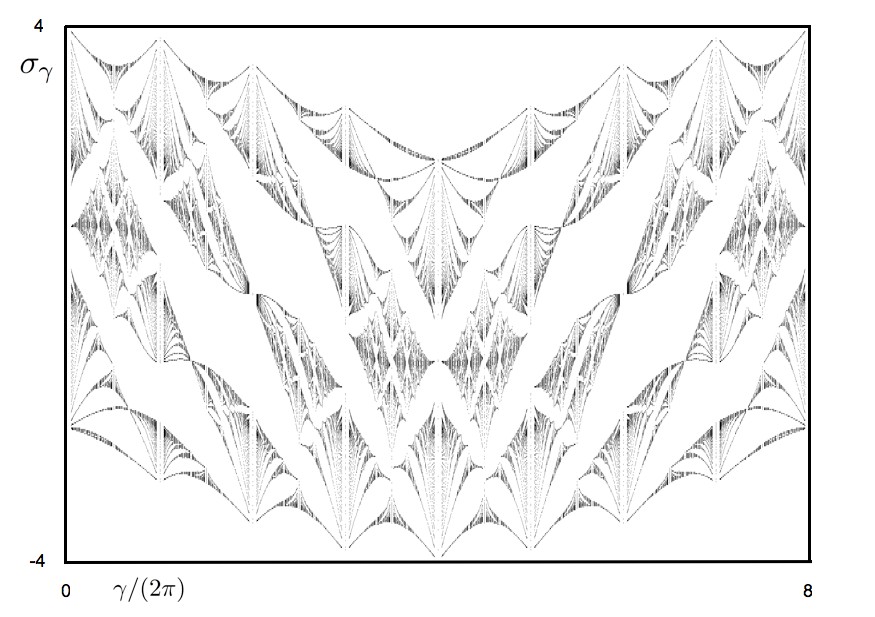
Figure 2: Hofstadter’s butterfly for the kagome lattice when $\omega=0$.

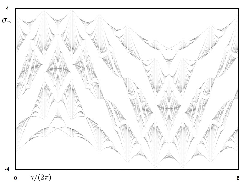
Figure 3: Hofstadter’s butterfly for the kagome lattice when $\omega=\pi/8$.

We notice that for fixed $\gamma=2\pi p/q$ the spectrum is composed of $3q$ (possibly not disjoint) bands, which are the images of

$$[0,1]\times[0,1]\ni(\theta_{1},\theta_{2})\mapsto\lambda_{p,q,\omega,\theta_{1},\theta_{2}}^{k}\,,\quad 1\leq k\leq 3q$$ (1.37)

where $\lambda_{p,q,\omega,\theta_{1},\theta_{2}}^{k}$ is the $k$th eigenvalue of $M_{p,q,\omega,\theta_{1},\theta_{2}}$.
Since the smallest positive integer for which the operator $Q_{\gamma,\omega}$ is invariant by the transformation $\gamma\mapsto\gamma+2\pi k$ is $k=8$, we plot in the vertical axis of Figures 2 and 3 the bands of the spectrum for

$$\frac{\gamma}{2\pi}=\frac{p}{q}\,,\quad p,q\text{ relatively prime and }0\leq p<8q\leq 400\,.$$

We first observe some symmetries in these butterflies and prove the proposition

Proposition 1.11.

Let $\sigma{{}_{\gamma},\omega}$ be the spectrum of $Q_{\gamma,\omega}$. We have

$$\sigma_{\gamma,\omega} \subset [-4,4]\,,$$ (1.38)

$$\sigma_{\gamma+16\pi,\omega} = \sigma_{\gamma,\omega}\hskip 35.56593pt(\text{translation invariance}),$$ (1.39)

$$e\in\sigma_{\gamma+8\pi,\omega} \Leftrightarrow -e\in\sigma_{\gamma,\omega}\quad(\text{translation anti-invariance}).$$ (1.40)

In the case when $\omega=0$, we have

$$\sigma_{-\gamma,0} = \sigma_{\gamma,0}\hskip 35.56593pt(\text{reflexion with respect to the axis $\gamma=0$}),$$ (1.41)

$$e\in\sigma_{8\pi-\gamma,0} \Leftrightarrow -e\in\sigma_{\gamma,0}\quad(\text{reflexion with respect to the point $(4\pi,0)$}).$$ (1.42)

In the case when $\omega=\pi/8$, we have

$$\sigma_{6\pi-\gamma,\frac{\pi}{8}} = \sigma_{\gamma,\frac{\pi}{8}}\hskip 35.56593pt(\text{reflexion with respect to the axis $\gamma=3\pi$}),$$ (1.43)

$$e\in\sigma_{-2\pi-\gamma,\frac{\pi}{8}} \Leftrightarrow -e\in\sigma_{\gamma,\frac{\pi}{8}}\quad(\text{reflexion with respect to the point $(-\pi,0)$}).$$ (1.44)

Second we note the presence of isolated points in $\sigma_{\frac{4\pi}{3},0}$, $\sigma_{\frac{8\pi}{3},0}$, $\sigma_{4\pi,0}$, $\sigma_{\pi,\frac{\pi}{8}}$, $\sigma_{3\pi,\frac{\pi}{8}}$, $\sigma_{\frac{7\pi}{3},\frac{\pi}{8}}$ and $\sigma_{-\frac{\pi}{3},\frac{\pi}{8}}$.
To see more precisely the last phenomenon, we plot in Figures 4b and 5 the bands of the spectra $\sigma_{4\pi,0}$, $\sigma_{\frac{4\pi}{3},0}$ and $\sigma_{\frac{8\pi}{3},0}$.

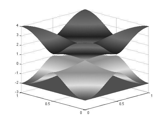
(a)

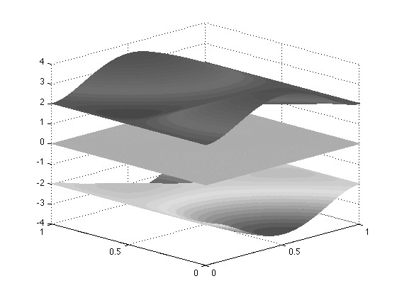
(b)

Figure 4: Spectrum bands of $Q_{\gamma,\omega}$ for (a) $(\gamma,\omega)=(0,0)$ and (b) $(\gamma,\omega)=(4\pi,0)$.

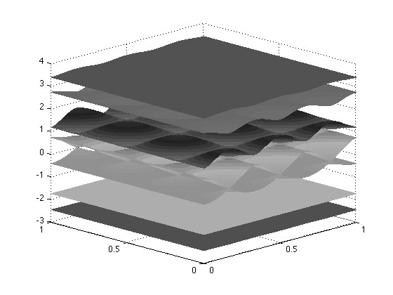
(a)

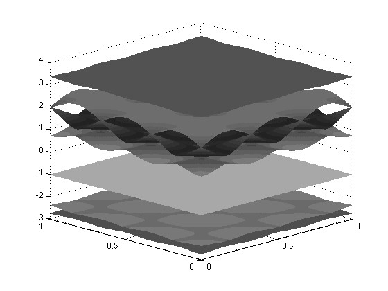
(b)

Figure 5: Spectrum bands of $Q_{\gamma,\omega}$ for (a) $(\gamma,\omega)=(4\pi/3,0)$ and (b) $(\gamma,\omega)=(8\pi/3,0)$.

Numerically it seems that the second, third and fourth bands of $\sigma_{\frac{4\pi}{3},0}$ are reduced to $\{-\sqrt{3}\}$, and that the third, fourth and fifth band of $\sigma_{\frac{8\pi}{3},0}$ are reduced to $\{-1\}$.
This leads to the definition

Definition 1.12.

Let $\lambda_{0}$ be a reel number and $n$ a positive integer. $\{\lambda_{0}\}$ is called a flat band of multiplicity $n$ of $\sigma_{\gamma,\omega}$ if the $k^{th}$ band of $\sigma_{\gamma,\omega}$ is reduced to $\{\lambda_{0}\}$ for exactly $n$ values of $k$.

One can easily compute the characteristic polynomials of the $3\times 3$ matrices $M_{0,1,0,\theta_{1},\theta_{2}}$ and $M_{2,1,0,\theta_{1},\theta_{2}}$. For the other cases, we use the symbolic computation software Mathematica and obtain

Proposition 1.13.

1. 1. $\{-2\}$ and $\{0\}$ are flat bands of multiplicity $1$ of $\sigma_{0,0}$ and $\sigma_{4\pi,0}$ respectively. $\sigma_{0,0}$ is composed of the three touching bands $\{-2\}$, $[-2,1]$ and $[1,4]$. $\sigma_{4\pi,0}$ is composed of the three disjoint bands $[-2\sqrt{3},-\sqrt{3}]$, $\{0\}$ and $[\sqrt{3},2\sqrt{3}]$.

   2. $\{-\sqrt{3}\}$ and $\{-1\}$ are flat bands of multiplicity $3$ of $\sigma_{\frac{4\pi}{3},0}$ and $\sigma_{\frac{8\pi}{3},0}$ respectively.

2. 1. $\{-\sqrt{2}\}$ and $\{-2\}$ are flat bands of multiplicity $2$ of $\sigma_{\pi,\frac{\pi}{8}}$ and $\sigma_{3\pi,\frac{\pi}{8}}$ respectively. $\sigma_{3\pi,\frac{\pi}{8}}$ is composed of the flat band $\{-2\}$ and the four touching bands
      $[1-\sqrt{6},1-\sqrt{3}]$, $[1-\sqrt{3},1]$, $[1,1+\sqrt{3}]$, and $[1+\sqrt{3},1+\sqrt{6}]$.

   2. $\{-\frac{\sqrt{6}+\sqrt{2}}{2}\}$ and $\{-\frac{\sqrt{6}-\sqrt{2}}{2}\}$ are flat bands of multiplicity $6$ of $\sigma_{\frac{7\pi}{3},\frac{\pi}{8}}$ and $\sigma_{-\frac{\pi}{3},\frac{\pi}{8}}$ respectively.

Remark 1.14.

This phenomenon does not occur for the square, triangular and hexagonal models.

Remark 1.15.

1. Proposition 1.13 ensures the existence of eigenvalues of infinite multiplicity for $Q_{\gamma,\omega}$ and $P^{kag}_{\gamma,\omega}$ for several values of $(\gamma,\omega)$.
2. Since the models $Q_{\gamma,\omega}$ and $P^{kag}_{\gamma,\omega}$ only take into account the interactions beetween nearest wells, and $\omega=\mathcal{O}(h)$ does not a priori vanish, the existence of eigenvalues for $Q_{\gamma,0}$ when $\gamma$ equals to $4\pi/3$, $8\pi/3$ or $4\pi$ does not imply the existence of eigenvalues for the corresponding initial Schrödinger operator $P_{h,A,V}$. However, Proposition 1.13 together with Theorem 1.5 ensure that, when the values of $A$ and $h$ lead to one of these values of $\gamma$, there exists $C>0$ suth that a part of the low lying spectrum of $P_{h,A,V}$ is included in an interval of length at most $C\,h^{\nicefrac{{3}}{{2}}}\exp(-S/h)$ and separated from the rest of the spectrum by intervals of lengh at least $C^{-1}\,h^{\nicefrac{{1}}{{2}}}\exp(-S/h)$.

Remark 1.16.

In the light of Proposition 1.13 we can state the following conjecture : if $\sigma_{2\pi p/q,\omega}$ contains a flat band for a real number $\omega$ and two relatively prime integers $p$ and $q$ with $q>0$, then its multiplicity is $q$.

An interesting question is to see how the invariances of the initial problem are conserved in the reduced model $p^{kag}$. The invariance by rotation of angle $\pi/3$ gave the application $\kappa$ on the indices $\alpha$, so the transpose application ${}^{t}\!\kappa(x,\xi)=(\xi,-x+\xi)$ is seen as the rotation of angle $-\pi/3$ on the phase space $\mathbb{R}_{x}\times\mathbb{R}_{\xi}$. We introduce the translations $\tilde{t}_{1}(x,\xi)=(x+2\pi)$ and $\tilde{t}_{2}(x,\xi)=(x,\xi+2\pi)$, and the symmetry $s(x,\xi)=(\xi,x)$. We then have

Proposition 1.17.

$$p^{kag}\circ\tilde{t}_{1}=p^{kag}\,,$$ (1.45)

$$p^{kag}\circ\tilde{t}_{2}=p^{kag}\,,$$ (1.46)

$$\left(\begin{array}[]{ccc}0&1&0\\ 0&0&1\\ 1&0&0\end{array}\right)^{-1}\left(p^{kag}\circ{}^{t}\!\kappa^{2}\right)\left(\begin{array}[]{ccc}0&1&0\\ 0&0&1\\ 1&0&0\end{array}\right) = p^{kag}\,,$$ (1.53)

$$\left(\begin{array}[]{ccc}0&0&1\\ 0&1&0\\ 1&0&0\end{array}\right)\overline{\left(p^{kag}\circ s\right)}\left(\begin{array}[]{ccc}0&0&1\\ 0&1&0\\ 1&0&0\end{array}\right) = p^{kag}\,.$$ (1.60)

Remark 1.18.

1. The invariance by the rotation of angle $\pi/3$ seems lost, but fortunately the action of the group generated by $\tilde{t}_{1}$, $\tilde{t}_{2}$, $s$ and ${}^{t}\!\kappa^{2}$ on the set of the microlocal wells, which are at energy $\lambda$ the connected components of $\{(x,\xi);\,\det(\lambda\,I_{3}-p^{kag}(x,\xi,0,\omega))=0\}$, is transitive.
2. As shown in [Ker95], the invariances of $p^{kag}$ give operators commuting with $P_{\gamma,\omega}^{kag}$.
We will develop these points in a further work joint with B.Helffer and devoted to the microlocal study of $P^{kag}_{\gamma,\omega}$.

Outline of the article

This article is organized as follows:

• In Section 2 we present a general theorem on the Weyl quantization of periodical symbols.

• In Section 3 we review the cases of the square, triangular and hexagonal lattices. We describe and prove the symmetries of the corresponding spectra.

• In Section 4 we study the properties of the kagome lattice and we construct a family of potentials invariant by the symmetries of $\Gamma_{\triangle}$, whose minima are located in $\Gamma$.

• Section 5 is devoted to the semi-classical analysis of the low lying spectrum of $P_{h,A,V}$ for $h$ small. We derive the discrete operator $W_{\gamma}$ and prove Theorem 1.3.

• In Section 6, we study the properties of $W_{\gamma}$ and prove Theorem 1.5. We give the representation using the pseudo-differential operator acting on $L^{2}(\mathbb{R};\mathbb{C}^{3})$ and prove Theorem 1.6. We then study the case when $\gamma/(2\pi)$ is rational and prove Theorem 1.9. We end this article by proving Propositions 1.8, 1.11 and 1.13.

Ackowledgements : This article is a revisited version of the second part of J. Royo-Letelier’s PhD thesis (defended in June 2013 at the Université de Versailles Saint-Quentin-en-Yvelines) with B. Helffer as advisor and written with the help of P. Kerdelhué. We warmly thank B. Helffer for suggesting us this problem and for his precious help with the realization of this article. The second author thanks the Institute of Science and Technology Austria (IST Austria) in which she was staying as a post-doc while this article was finalized. The first author thanks P. Gamblin for useful conversations.

2 Quantization of periodical symbols

We first give a general theorem on the $\gamma$-quantization of a periodic symbol, which will be used to study the symmetries of the butterflies associated to the square, triangular, hexagonal and kagome models, and in the proofs of Theorems 1.5 and 1.6. This theorem was first established in [HS88a] and [Ker92] for Harper’s and triangular models, and under the restriction $0<\gamma<2\pi$. We present here a slightly different proof to avoid this restriction.

Let $n\in\mathbb{N}^{*}$ and $(\beta,\gamma)\mapsto p_{\beta,\gamma}$ be a function on $\mathbb{Z}^{2}\times\mathbb{R}^{*}$ with values in $M_{n}(\mathbb{C})$ such that :

$$\forall N\in\mathbb{N},~{}~{}\exists C_{N}>0,~{}~{}\forall(\beta,\gamma)\in\mathbb{Z}^{2}\times\mathbb{R}^{*}, |p_{\beta,\gamma}|\leq C_{N}(1+\beta_{1}+\beta_{2})^{-N}\,,$$ (2.1)

$$\forall(\beta,\gamma)\in\mathbb{Z}^{2}\times\mathbb{R}^{*}, p_{-\beta,\gamma}=p^{*}_{\beta,\gamma}\,.$$ (2.2)

We define the symbol

$$p(x,\xi,\gamma)=\sum_{\beta\in\mathbb{Z}^{2}}p_{\beta,\gamma}\,e^{i(\beta_{1}x+\beta_{2}\xi)}\$$ (2.3)

and its Weyl quantization $P_{\gamma}$ introduced in (1.12). A straightforward computation gives that $P_{\gamma}$ acts on $L^{2}(\mathbb{R};\,\mathbb{C}^{n})$ by

$$P_{\gamma}\,u(x)=\sum_{\beta\in\mathbb{Z}^{2}}p_{\beta,\gamma}\,e^{i\frac{\gamma}{2}\beta_{1}\beta_{2}}\,e^{i\beta_{1}x}\,u(x+\beta_{2}\gamma)\,.$$ (2.4)

We also consider the discrete operator

$$Q_{\gamma}=\sum_{\beta\in\mathbb{Z}^{2}}p_{\beta,\gamma}\,e^{i\frac{\gamma}{2}\beta_{1}\beta_{2}}\,\tau_{1}^{\beta_{1}}\tau_{2}^{\beta_{2}}$$

where $\tau_{1}$ and $\tau_{2}$ are the discrete magnetic translations defined in (1.11), and $A_{\gamma}$ the infinite matrix defined by

$$\left(A_{\gamma}\right)_{\alpha,\beta}=e^{-i\frac{\gamma}{2}\alpha\wedge\beta}p_{\alpha-\beta,\gamma}$$

and acting on $\ell^{2}(\mathbb{Z}^{2};\,\mathbb{C}^{n})$ by

$$\left(A_{\gamma}v\right)_{\alpha}=\sum_{\beta\in\mathbb{Z}^{2}}\left(A_{\gamma}\right)_{\alpha,\beta}\,v_{\beta}\,.$$

Theorem 2.1.

$A_{\gamma}$ and $Q_{\gamma}$ are unitary equivalent. $P_{\gamma}$, $A_{\gamma}$ and $Q_{\gamma}$ have the same spectrum.

Proof. The first hypothesis anables to prove the convergence of the series defining $p$, $A_{\gamma}$ and $Q_{\gamma}$, and the second one gives the self-adjointness of $A_{\gamma}$, $Q_{\gamma}$ and $P_{\gamma}$.

$Q_{\gamma}$ acts on $\ell^{2}(\mathbb{Z}:\mathbb{C}^{n})$ by

$$Q_{\gamma}u(\alpha) = \sum_{\beta\in\mathbb{Z}^{2}}p_{\beta,\gamma}\,e^{-i\frac{\gamma}{2}\beta_{1}\beta_{2}}e^{i\gamma\alpha_{1}\beta_{2}}u_{\alpha-\beta}$$

$$= \sum_{\beta\in\mathbb{Z}^{2}}p_{\alpha-\beta,\gamma}\,e^{i\frac{\gamma}{2}(\alpha_{1}\alpha_{2}-\beta_{1}\beta_{2}-\alpha\wedge\beta)}u_{\beta}$$

so $A_{\gamma}$ and $Q_{\gamma}$ are unitary equivalent.

The operator $P_{\gamma}$ commutes with the translation $u(\cdot)\mapsto u(\cdot-2\pi)$, so Floquet theory applies and the spectrum of $P_{\gamma}$ is the union over $\theta\in\mathbb{R}$ of the spectra of the operators $P^{\theta}_{\gamma}$ acting on the space $\displaystyle\left\{u\in L_{\text{loc}}^{2}(\mathbb{R};\mathbb{C}^{n})\,;\,u(\cdot+2\pi)=e^{i2\pi\theta}u(\cdot)\,a.e.\right\}$ by

$$P^{\theta}_{\gamma}\,u(x)=\sum_{\beta\in\mathbb{Z}^{2}}p_{\beta,\gamma}\,e^{i\frac{\gamma}{2}\beta_{1}\beta_{2}}\,e^{i\beta_{1}x}\,u(x+\beta_{2}\gamma)\,.$$

We notice that $P^{\theta}_{\gamma}$ has the same spectrum than its conjugate $\tilde{P}^{\theta}_{\gamma}=e^{-i\theta x}P^{\theta}_{\gamma}\,e^{i\theta x}$ acting on $L^{2}(\mathbb{R}/2\pi\mathbb{Z};\mathbb{C}^{n})$ by

$$\tilde{P}^{\theta}_{\gamma}\,u(x)=\sum_{\beta\in\mathbb{Z}^{2}}p_{\beta,\gamma}\,e^{i\frac{\gamma}{2}\beta_{1}\beta_{2}}\,e^{i\beta_{1}x}\,e^{i\gamma\beta_{2}\theta}u(x+\beta_{2}\gamma)\,.$$

The union over $\theta\in\mathbb{R}$ of the spectra of the operators $\tilde{P}^{\theta}_{\gamma}$ is the union over $\theta\in[0,2\pi/\gamma]$ (or $\theta\in[2\pi/\gamma,0]$ in the case when $\gamma<0$) of these spectra. Hence the spectrum of $P_{\gamma}$ is the spectrum of the operator $\check{P}_{\gamma}$ acting on $L^{2}(\mathbb{R}/2\pi\mathbb{Z}\times\mathbb{R}/\frac{2\pi}{\gamma}\mathbb{Z};\mathbb{C}^{n})$ by

$$\check{P}_{\gamma}u(x,\theta)=\sum_{\beta\in\mathbb{Z}^{2}}p_{\beta,\gamma}\,e^{i\frac{\gamma}{2}\beta_{1}\beta_{2}}\,e^{i\beta_{1}x}\,e^{i\gamma\beta_{2}\theta}u(x+\beta_{2}\gamma,\theta)\,.$$

We define the unitary Fourier transform $\mathcal{F}$ mapping $L^{2}((\mathbb{R}/2\pi\mathbb{Z})\times(\mathbb{R}/\frac{2\pi}{\gamma}\mathbb{Z});\mathbb{C}^{n})$ on $\ell^{2}(\mathbb{Z}^{2};\mathbb{C}^{n})$ by

$$(\mathcal{F}u)_{\alpha}=\frac{\gamma^{\nicefrac{{1}}{{2}}}}{2\pi}\int\!\!\!\int e^{-i(\alpha_{1}x+\gamma\alpha_{2}\theta)}u(x,\theta)\,dx\,d\theta$$

and a straightforward computation gives

$$\mathcal{F}\,\check{P}_{\gamma}=Q_{\gamma}\,\mathcal{F}\,.$$

So $\check{P}_{\gamma}$ and $Q_{\gamma}$ are unitary equivalent. Hence $P_{\gamma}$ and $Q_{\gamma}$ have the same spectrum.
∎

3 The square, triangular and hexagonal lattices

3.1 Presentation of the models

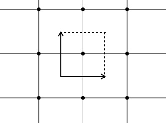
(a)

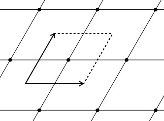
(b)

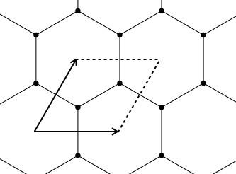
(c)

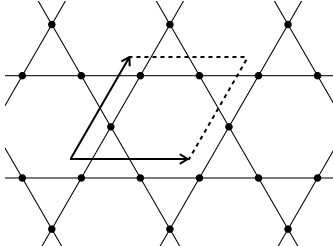
(d)

Figure 6: (a) square, (b) triangular, (c) hexagonal and (d) kagome lattices. In each case we had drawn a fundamental domain of the Bravais lattice. The points of the lattice correspond to the minima of the electric potential.

The spectral properties of $P_{h,A,V}$ have been studied for the square, triangular and hexagonal lattices. When plotting the spectrum as a function of $\gamma$, we obtain a picture with several symmetries, which are determined by the symmetries of the lattice. In the case of the square lattice, we get the famous Hofstadter butterfly. In this section we review and prove the symmetries of these spectra using the pseudo-differential operators associated with these lattices. We recall that the symbols corresponding to the square, triangular and hexagonal lattices are respectively

$$p^{\Box}(x,\xi) = \cos x+\cos\xi\,,$$ (3.1)

$$p^{\triangle}(x,\xi) = \cos x+\cos\xi+\cos(x-\xi)\,,$$ (3.2)

$$p^{hex}(x,\xi) = \left(\begin{array}[]{cc}0&1+e^{ix}+e^{i\xi}\\ 1+e^{-ix}+e^{-i\xi}&0\end{array}\right)\,.$$ (3.5)

The size of the matrix is the number of points of the lattice in each fundamental domain. The number of terms of the form $e^{i(ax+b\xi)}$ is the product of this number by the number of nearest neighbours of each point of the lattice.

To study the symmetries of the Hofstadter’s butterflies associated with each model, we will use the following direct consequence of Theorem 2.1.

Proposition 3.1.

Let $n\in\mathbb{N}^{*}$ and $\beta\mapsto p_{\beta}$ be a function on $\mathbb{Z}^{2}$ (here $p_{\beta}$ does not depend on $\gamma$) with values in $M_{n}(\mathbb{C})$ satisfying (2.1) and (2.2). Consider the symbol $p(x,\xi)$ defined in (2.3), its Weyl quantization $P_{\gamma}$ and denote by $\sigma(P_{\gamma})$ the spectrum of $P_{\gamma}$. We have:

$$\text{ If }p_{\beta}=0\text{ for }\beta_{1}\text{ and }\beta_{2}\text{ odd, then \, } \forall\gamma\in\mathbb{R}\,,\sigma(P_{\gamma+2\pi})=\sigma(P_{\gamma})\,.$$ (3.6)

$$\text{ If }p_{\beta}=0\text{ for }\beta_{1}\text{ and }\beta_{2}\text{ even, then } \forall\gamma\in\mathbb{R}\,,\sigma(P_{\gamma+2\pi})=-\sigma(P_{\gamma})\,.$$ (3.7)

Remark 3.2.

Property (3.6) applies to the Harper model $p^{\Box}$ and the hexagonal model $\displaystyle p^{hex}$. Property (3.7) applies to the triangular model $p^{\triangle}$.

Proof. First we notice that the magnetic translations $\tau_{1}$ and $\tau_{2}$ defined in (1.11) don’t change when we replace $\gamma$ by $\gamma+2\pi$. Hence Theorem 2.1 gives

$$\sigma(P_{\gamma+2\pi})=\sigma\left({\rm Op}^{W}_{\gamma}\left(\sum_{\beta\in\mathbb{Z}^{2}}(-1)^{\beta_{1}\beta_{2}}p_{\beta}\,e^{i(\beta_{1}x+\beta_{2}\xi)}\right)\right)\,,$$

so (3.6) is proved.

Since the application $(x,\xi)\mapsto(x+\pi,\xi+\pi)$ is affine and symplectic the operators

$${\rm Op}_{\gamma}^{W}\left(\sum_{\beta\in\mathbb{Z}^{2}}(-1)^{\beta_{1}\beta_{2}}p_{\beta}\,e^{i(\beta_{1}x+\beta_{2}\xi)}\right)\quad\text{ and }\quad{\rm Op}_{\gamma}^{W}\left(\sum_{\beta\in\mathbb{Z}^{2}}(-1)^{\beta_{1}\beta_{2}}p_{\beta}\,e^{i(\beta_{1}(x+\pi)+\beta_{2}(\xi+\pi))}\right)$$

are unitary equivalent. Then,

$$\sigma\left(\sum_{\beta\in\mathbb{Z}^{2}}(-1)^{\beta_{1}\beta_{2}}p_{\beta}\,e^{i(\beta_{1}x+\beta_{2}\xi)}\right) = \sigma\left(\sum_{\beta\in\mathbb{Z}^{2}}(-1)^{\beta_{1}\beta_{2}}p_{\beta}\,e^{i(\beta_{1}(x+\pi)+\beta_{2}(\xi+\pi))}\right)$$

$$= -\sigma\left(\sum_{\beta\in\mathbb{Z}^{2}}(-1)^{(\beta_{1}+1)(\beta_{2}+1)}p_{\beta}\,e^{i(\beta_{1}x+\beta_{2}\xi)}\right)\,,$$

which yields (3.7).
∎

3.2 The square lattice

The square lattice is the Bravais lattice associated with the basis $\{(1,0),(0,1)\}$ of $\mathbb{R}^{2}$. Each point of the lattice has 4 nearest neighbours for the Euclidean distance. One of the models used in this case is the discrete operator $L^{\Box}_{\gamma}$ defined on $\ell^{2}(\mathbb{Z}^{2},\mathbb{C})$ by

$$L^{\Box}_{\gamma}=\frac{1}{2}\left(\tau_{1}+\tau_{1}^{*}+\tau_{2}+\tau_{2}^{*}\right)\,,$$ (3.8)

where $\tau_{1},\tau_{2}$ are the discrete magnetic translations defined in (1.11).

Using a partial Floquet theory, we are led to the study of the spectrum of a family (parametrized by $\theta_{2}$) of discrete Schrödinger operators $L^{\Box}_{\gamma,{\theta_{2}}}$ acting over $\ell^{2}(\mathbb{Z})$ by

$$(L^{\Box}_{\gamma,{\theta_{2}}}v)_{n}=\frac{v_{n+1}+v_{n-1}}{2}+V_{{\theta_{2}}}(n)v_{n}\,,$$ (3.9)

where $V_{\theta_{2}}(n)=\cos\left(\gamma n+\theta_{2}\right)$ is the discrete potential.

Notice that $L^{\Box}_{\gamma,{\theta_{2}+\gamma}}$ is unitary equivalent with $L^{\Box}_{\gamma,{\theta_{2}}}$. When $\gamma/(2\pi)$ is irrational, the spectrum of $L^{\Box}_{\gamma,{\theta_{2}}}$ does not depend on ${\theta_{2}}$ (see [HS88a], §1). This is no longer the case when $\gamma/(2\pi)$ is rational. In 1976 Hofstadter performed a formal study of the spectrum of $L^{\Box}_{\gamma,{\theta_{2}}}$ as a function of $\gamma/(2\pi)\in\mathbb{Q}$ ([Hof76]). His approach suggests a fractal structure for the spectrum and leads to Hofstadter’s butterfly. The method consists in studying numerically the case $\gamma=2\pi p/q$, with $p,q\in\mathbb{N}$ relative primes. Hofstadter observed that in this case, the spectrum is formed of $q$ bands which can only touch at their boundary. Hofstadter’s butterfly is obtained by placing in the $y$-axis of a graph the bands of the spectrum (see Figure 7a). Moreover, Hofstadter derived rules for the configuration of the bands related to the expansion of $p/q$ as continued fraction. This configuration strongly suggests the Cantor structure of the spectrum of $L^{\Box}_{\gamma,{\theta_{2}}}$ when $\gamma/(2\pi)$ is irrational. A longtime open problem, proposed by Kac and Simon in the 80’s and called the “Ten Martinis problem” ([Sim], Problem 4), was to prove that for irrational $\gamma/(2\pi)$, the spectrum of $L^{\Box}_{\gamma}$ is a Cantor set. After many efforts starting with the article of Bellissard and Simon in 1982 ([BS82]), the problem was finally solved in 2009 by Avila and Jitomirskaya ([AJ09]).

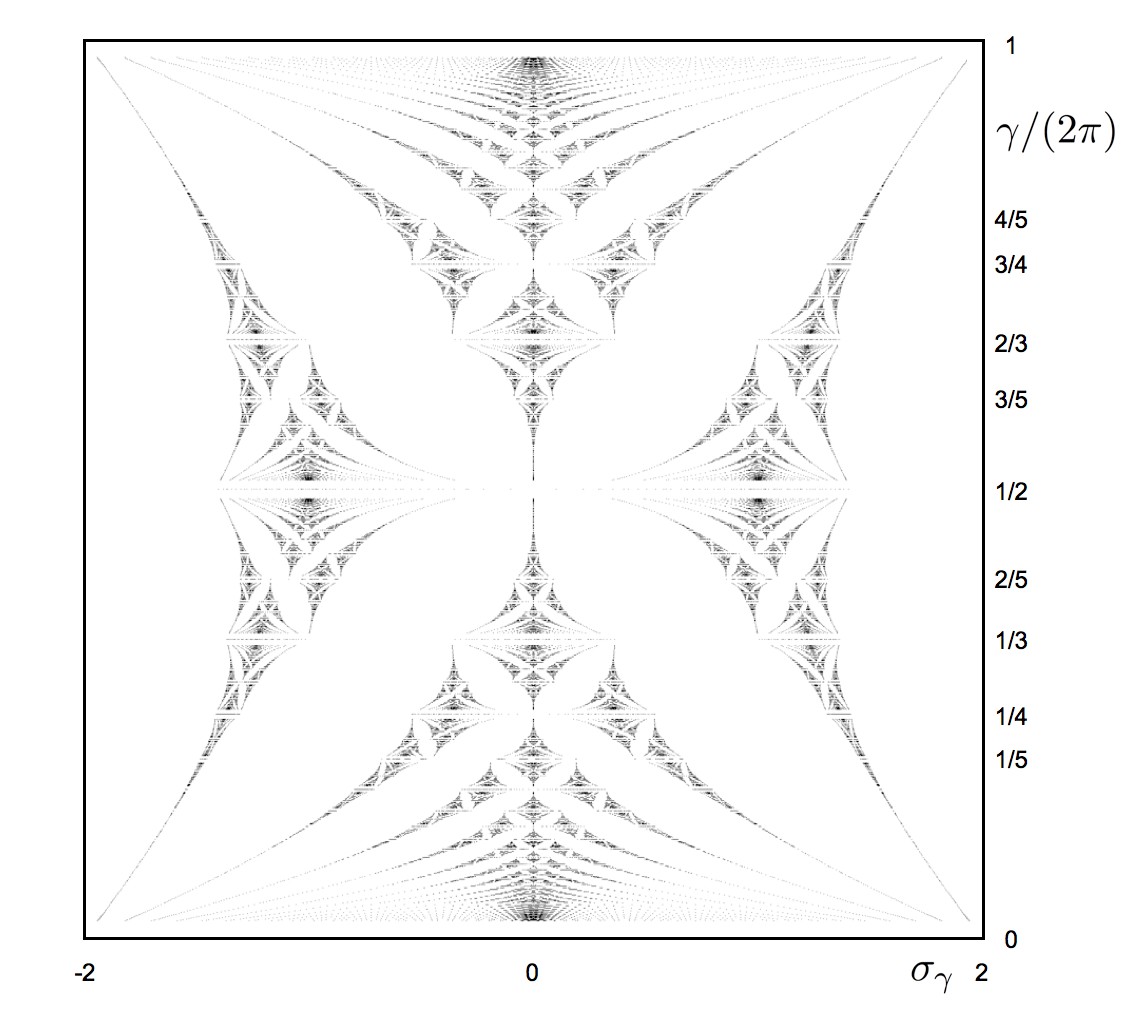
(a)

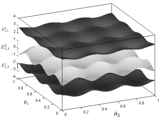
(b)

Figure 7: (a) The spectrum of $P^{\Box}_{\gamma}$ corresponding to the square lattice (Hofstadter’s butterfly). (b) Energy bands for $\gamma=2\pi/3$.

In order to compute the spectrum of $L^{\Box}_{\gamma}$ for $\gamma=2\pi p/q$, we may use again the Floquet theory. Introducing the Floquet condition $v_{n+q}=e^{i2\pi\theta_{1}q}v_{n}$, we are led to the computation of the eigenvalues of a family (parametrized by $\theta_{1}$ and $\theta_{2}$). Denoting $\sigma^{\Box}_{\gamma}=\sigma(L^{\Box}_{\gamma})$ we obtain

$$\sigma^{\Box}_{\gamma}=\bigcup_{\theta_{1},\theta_{2}\in[0,1]}\sigma(M^{\Box}_{p,q,\theta_{1},\theta_{2}})\,,$$

where

$$M^{\Box}_{p,q,\theta_{1},\theta_{2}}=\frac{1}{2}\left(e^{i2\pi\theta_{1}}K_{q}+e^{-i2\pi\theta_{1}}K_{q}^{*}+e^{i2\pi\theta_{2}}J_{p,q}+e^{-i2\pi\theta_{2}}J_{p,q}^{*}\right)\,$$

with $J_{p,q}$, $K_{q}$ defined in (1.33).

For $1\leq k\leq q$ the $k$th band of $\sigma^{\Box}_{\gamma}$ is given by the image of

$$E_{p,q}^{k}:[0,1]\times[0,1]\to\mathbb{R}\,,\qquad(\theta_{1},\theta_{2})\mapsto\lambda_{p,q,\theta_{1},\theta_{2}}^{k}\,,$$ (3.10)

where $\lambda_{p,q,\theta_{1},\theta_{2}}^{k}$ is the $k$th eigenvalue of $M^{\Box}_{p,q,\theta_{1},\theta_{2}}$ (see Figure 7b).

In [HS88a], §1, it was proved that $L^{\Box}_{\gamma}$ is unitary equivalent with the pseudo-differential operator $P^{\Box}_{\gamma}$ defined in (2.4) for $p^{\Box}$ given in (3.1). Helffer and Sjöstrand developed in [HS88a, HS89, HS90] sophisticated techniques (inspired by the work of the physicist Wilkinson ([Wil84]) to study the operator $P^{\Box}_{\gamma}$. In particular, they justified in various regimes the approximation for the low spectrum of $P_{h,A,V}$ by the spectrum of $P^{\Box}_{\gamma}$.

When plotting $\sigma^{\Box}_{\gamma}$ as a function of $\gamma$ (see Figure 7a), we observe the following properties.

Proposition 3.3.

$$\sigma^{\Box}_{\gamma} \subset [-2,2]\,,$$ (3.11)

$$\sigma^{\Box}_{\gamma+2\pi} = \sigma^{\Box}_{\gamma}\hskip 27.03003pt(\text{translation invariance}),$$ (3.12)

$$\sigma^{\Box}_{-\gamma} = \sigma^{\Box}_{\gamma}\hskip 27.03003pt(\text{reflexion with respect to the axis $\gamma=0$}),$$ (3.13)

$$\sigma^{\Box}_{2\pi-\gamma} = \sigma^{\Box}_{\gamma}\qquad(\text{reflexion with respect to the axis $\gamma=\pi$}),$$ (3.14)

$$-e\in\sigma^{\Box}_{\gamma} \Leftrightarrow e\in\sigma^{\Box}_{\gamma}\quad(\text{reflexion with respect to the axis $e=0$})\,.$$ (3.15)

Proof. The definition of $p^{\Box}(x,\xi)$ together with the fact that the Weyl quantizations of $e^{ix}$, $e^{-ix}$, $e^{i\xi}$, $e^{-i\xi}$ are unitary operators yield (3.11). Property (3.6) gives (3.12). We obtain (3.13) noticing that

$$P^{\Box}_{-\gamma}={\rm Op}^{W}_{-\gamma}\left(p^{\Box}(x,\xi)\right)={\rm Op}^{W}_{\gamma}\left(p^{\Box}(x,-\xi)\right)={\rm Op}^{W}_{\gamma}\left(p^{\Box}(x,\xi)\right)=P^{\Box}_{\gamma}\,.$$

Properties (3.12) and (3.13) imply (3.14). Finally, we have that

$$p^{\Box}(x+\pi,\xi+\pi)=-p^{\Box}(x,\xi)$$

so $P^{\Box}_{\gamma}$ and $-P^{\Box}_{\gamma}$ are conjugate by the unitary operator $u\mapsto e^{\frac{i}{\gamma}\pi\cdot}u(\cdot-\pi)$. This yields (3.15).
∎

3.3 The triangular lattice

The triangular lattice is the Bravais lattice associated with the basis $\{(1,0),(\nicefrac{{1}}{{2}},-\nicefrac{{\sqrt{3}}}{{2}})\}$. Each point of the lattice has 6 nearest neighbors for the Euclidean distance. This case was studied by Claro and Wannier in [CW79]. These authors exhibit an analogous structure to the case of the square lattice. In the case $\gamma=2\pi p/q$, with $p,q\in\mathbb{N}$ relative primes, the spectrum is formed of $q$ bands which can only touch at their boundary (see Figure 8a). In [Ker92], the first author studied rigorously the operator $P_{h,A,V}$ in this case. He justified the reduction to the pseudo-differential operator $P_{\gamma}^{\triangle}$ defined in (2.4) with $p^{\triangle}$ given in (3.2).

As in the case of the square lattice discussed before, when $\gamma=2\pi p/q$ the spectrum can be computed by considering the family of matrices in $M_{q}(\mathbb{C})$ defined by

$$M^{\triangle}_{p,q,\theta_{1},\theta_{2}} = \frac{1}{2}\left(\ e^{i2\pi\theta_{1}}K_{q}+e^{-i2\pi\theta_{1}}K_{q}^{*}+e^{i2\pi\theta_{2}}J_{p,q}+e^{-i2\pi\theta_{2}}J_{p,q}^{*}\right.$$

$$\left.+e^{-i\pi\nicefrac{{p}}{{q}}}e^{i2\pi(\theta_{1}+\theta_{2})}J_{p,q}K_{q}+e^{-i\pi\nicefrac{{p}}{{q}}}e^{-i2\pi(\theta_{1}+\theta_{2})}J_{p,q}^{*}K_{q}^{*}\right)\,.$$

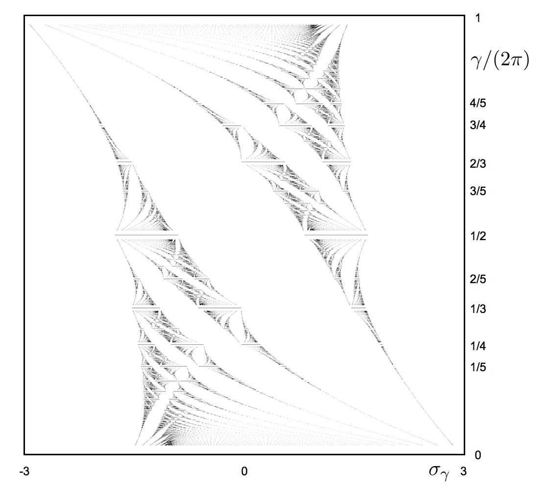
(a)

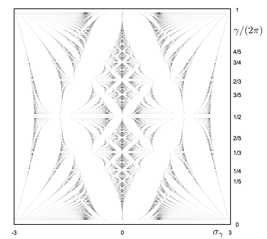
(b)

Figure 8: Hofstadter’s butterfly for (a) the triangular and (b) the hexagonal lattices.

Let $\sigma^{\triangle}_{\gamma}$ be the spectrum of $P^{\triangle}_{\gamma}$. When plotting $\sigma^{\triangle}_{\gamma}$ as a function of $\gamma$ (see Figure 8a), we observe the following properties.

Proposition 3.4.

$$\sigma^{\triangle}_{\gamma} \subset [-3,3]\,,$$ (3.16)

$$\sigma^{\triangle}_{\gamma+4\pi} = \sigma^{\triangle}_{\gamma}\hskip 27.03003pt(\text{translation invariance}),$$ (3.17)

$$\sigma^{\triangle}_{-\gamma} = \sigma^{\triangle}_{\gamma}\hskip 27.03003pt(\text{reflexion with respect to the axis $\gamma=0$}),$$ (3.18)

$$e\in\sigma^{\triangle}_{2\pi-\gamma} \Leftrightarrow -e\in\sigma^{\triangle}_{\gamma}\qquad(\text{reflexion with respect to the point $(0,\pi)$})\,.$$ (3.19)

Proof. The definition of $p^{\triangle}(x,\xi)$ together with the fact that the Weyl quantizations of $e^{ix}$, $e^{-ix}$, $e^{i\xi}$, $e^{-i\xi}$, $e^{i(x-\xi)}$ and $e^{-i(x-\xi)}$ are unitary operators yield (3.16). Property (3.17) comes from Proposition 3.1. We have that

$${\rm Op}^{W}_{-\gamma}\left(p^{\triangle}(x,\xi)\right)={\rm Op}^{W}_{\gamma}\left(p^{\triangle}(x,-\xi)\right)={\rm Op}^{W}_{\gamma}\left(\cos x+\cos\xi+\cos(x+\xi)\right)\,.$$

The application $(x,\xi)\mapsto(x,-x+\xi)$ is linear symplectic so ${\rm Op}^{W}_{\gamma}\left(\cos x+\cos\xi+\cos(x+\xi)\right)$ and

$${\rm Op}^{W}_{\gamma}\left(\cos x+\cos(-x+\xi)+\cos(x+(-x+\xi))\right)={\rm Op}^{W}_{\gamma}\left(p^{\triangle}(x,\xi)\right)$$

are unitary equivalent. This yields (3.18). Proposition 3.1 implies that $e\in\sigma^{\triangle}_{2\pi-\gamma}$ if and only if $-e\in\sigma^{\triangle}_{-\gamma}$. This, together with (3.18), yield (3.19).
∎

3.4 The hexagonal lattice

The hexagonal lattice is not a Bravais lattice, but is a discrete subset of $\mathbb{R}^{2}$ invariant under the rotation of angle $\pi/3$ and translation along a triangular lattice, and containing two points per fundamental domain of this lattice. Each point of the lattice has 3 nearest neighbors. This case was also rigorously studied by the first author in [Ker92] and [Ker95]. We remark that this configuration corresponds to a charged particle in a graphene sheet submitted to a transverse magnetic field ([Mon13], §6). This case acquired a new interest after the 2010 Nobel Prize in Physics awarded to Geim and Novoselov for their experiments involving graphene ([Gei11, Nob, Nov11]). In the case of a hexagonal lattice, thefirst author justified the reduction to a pseudo-differential operator $P_{\gamma}^{hex}$ defined in (2.4) with $p^{hex}$ given in (3.5).

In the case when $\gamma=2\pi p/q$, the spectrum can be numerically computed by diagonalizing the hermitian matrices in $M_{2q}(\mathbb{C})$ defined by

$$M^{{hex}}_{p,q,\theta_{1},\theta_{2}}=\left(\begin{array}[]{c|c}&\\ 0_{q}&I_{q}+e^{i{\theta_{1}}}K_{q}+e^{-i{\theta_{2}}}J^{*}_{p,q}\\ &\\ \hline\cr&\\ I_{q}+e^{-i{\theta_{1}}}K_{q}^{*}+e^{i{\theta_{2}}}J_{p,q}&0_{q}\\ &\end{array}\right)\,.$$

Let $\sigma^{hex}_{\gamma}$ be the spectrum of $P_{\gamma}^{hex}$. When plotting $\sigma^{hex}_{\gamma}$ as a function of $\gamma$ (see Figure 8b), we observe the following properties.

Proposition 3.5.

$$\sigma^{hex}_{\gamma} \subset [-3,3]\,,$$ (3.20)

$$\sigma^{hex}_{\gamma+2\pi} = \sigma^{hex}_{\gamma}\hskip 27.03003pt\text{ (translation invariance), }$$ (3.21)

$$\sigma^{hex}_{-\gamma} = \sigma^{hex}_{\gamma}\hskip 27.03003pt\text{ (reflexion with respect to the axis $\gamma=0$}),$$ (3.22)

$$\sigma^{hex}_{2\pi-\gamma} = \sigma^{hex}_{\gamma}\qquad\text{ (reflexion with respect to the axis $\gamma=\pi$}),$$ (3.23)

$$-e\in\sigma^{hex}_{\gamma} \Leftrightarrow e\in\sigma^{hex}_{\gamma}\quad(\text{reflexion with respect to the axis $e=0$})\,.$$ (3.24)

Proof. We obtain (3.20) observing that

$$p^{{hex}}(x,\xi)=\left(\begin{array}[]{cc}0&1\\ 1&0\end{array}\right)+\left(\begin{array}[]{cc}0&e^{ix}\\ e^{-ix}&0\end{array}\right)+\left(\begin{array}[]{cc}0&e^{i\xi}\\ e^{-i\xi}&0\end{array}\right)$$

and that the Weyl quantizations of

$$\left(\begin{array}[]{cc}0&1\\ 1&0\end{array}\right)\,,\qquad\left(\begin{array}[]{cc}0&e^{ix}\\ e^{-ix}&0\end{array}\right)\quad\text{ and }\quad\left(\begin{array}[]{cc}0&e^{i\xi}\\ e^{-i\xi}&0\end{array}\right)$$

are unitary operators. Property (3.21) comes from Proposition 3.1. Notice that

$${\rm Op}^{W}_{-\gamma}\left(p^{hex}(x,\xi)\right)={\rm Op}^{W}_{\gamma}\left(p^{hex}(x,-\xi)\right)={\rm Op}^{W}_{\gamma}\left(\begin{array}[]{cc}0&1+e^{ix}+e^{-i\xi}\\ 1+e^{-ix}+e^{i\xi}&0\end{array}\right)$$

and let $\Gamma$ be the operator defined by $\Gamma u(x)=\overline{u(-x)}$. It is classical and easy to check that if $q$ is a symbol, $\Gamma\,{\rm Op}^{W}_{\gamma}q(x,\xi)\,\Gamma={\rm Op}^{W}_{\gamma}\overline{q(-x,\xi)}$. This gives

$$\Gamma\,{\rm Op}^{W}_{\gamma}\left(\begin{array}[]{cc}0&1+e^{ix}+e^{-i\xi}\\ 1+e^{-ix}+e^{i\xi}&0\end{array}\right)\,\Gamma={\rm Op}^{W}_{\gamma}p^{hex}(x,\xi)\,,$$

which yields (3.22). Property (3.23) follows from (3.21) and (3.22). Finally, noting that

$$\left(\begin{array}[]{cc}-1&0\\ 0&1\end{array}\right)p^{hex}(x,\xi)\left(\begin{array}[]{cc}-1&0\\ 0&1\end{array}\right)=-p^{hex}(x,\xi)\,$$

we obtain

$$\left(\begin{array}[]{cc}-1&0\\ 0&1\end{array}\right)P^{hex}_{\gamma}\left(\begin{array}[]{cc}-1&0\\ 0&1\end{array}\right)=-P^{hex}_{\gamma}\,,$$

which yields (3.24).
∎

4 The kagome lattice

4.1 The group of symmetries of $\Gamma$

We now study the properties of the kagome lattice and its group of symmetries $\mathcal{G}$.

For $\alpha\in\mathbb{Z}^{2}$ we set $t^{\alpha}=t_{1}^{\alpha_{1}}t_{2}^{\alpha_{2}}$. We then have

$$rt^{\alpha}=t^{\kappa(\alpha)}r\,,$$ (4.1)

where $\kappa$ is given in (1.5). We also notice that

$$\kappa^{6}=id_{\mathbb{Z}^{2}}\quad\text{ and }\quad\kappa(\alpha)\wedge\kappa(\beta)=\alpha\wedge\beta\,,$$ (4.2)

where $\wedge$ is the cross product $\alpha\wedge\beta=\alpha_{1}\beta_{2}-\alpha_{2}\beta_{1}$. Then we easily obtain

Proposition 4.1.

The kagome lattice is invariant by the maps in $\mathcal{G}$ and for every $m,n\in\Gamma$ there exists $g\in\mathcal{G}$ such that $g(m)=n$.

4.2 Construction of kagome potentials

We call $V:\mathbb{R}^{2}\to\mathbb{R}$ a kagome potential if it satisfies Hypothesis 1.1. It is rather easy to define such a potential, but more interesting is to give explicit examples in the class of trigonometric polynomials, which leaves open the possibility to realize experimentally these potentials with lasers (see for example [DFE⁺05] and [SBE⁺04]).

Remembering the definitions of the vectors $\nu_{j}$ from (1.2), we denote by $\nu^{\perp}$ the vector deduced from $\nu$ by a rotation of $\nicefrac{{\pi}}{{2}}$ and for $j\in\{1,3,5\}$ we define (see Figure 9)

$$\mu_{j}=\sqrt{3}\,\nu_{j}^{\perp}\,.$$ (4.3)

For $j=1,3,5$ we set $\phi_{j}=3\pi/2$ and define the potentials $V_{j}:\mathbb{R}^{2}\to\mathbb{R}$ as

$$V_{j}(x)=\left[\cos\left(x\cdot\pi\mu_{j}+\phi_{j}\right)+2\cos\left(\frac{x\cdot\pi\mu_{j}+\phi_{j}}{3}\right)\right]^{2}\,,$$ (4.4)

and $\tilde{V}$ as

$$\tilde{V}=V_{1}+V_{3}+V_{5}\,.$$ (4.5)

A straightforward computation gives

Proposition 4.2.

The function

$$V=-\tilde{V}+\|\tilde{V}\|_{\infty}\,,$$ (4.6)

satisfies (1.7) and (1.9) and has local minima at the points of the kagome lattice.

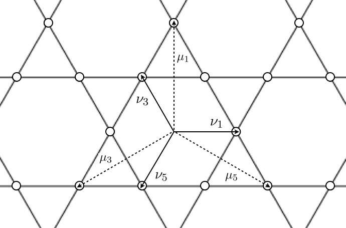
Figure 9: Vectors $\nu_{1}$, $\nu_{3}$, $\nu_{5}$, $\mu_{1}$, $\mu_{3}$ and $\mu_{5}$.

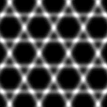
(a)

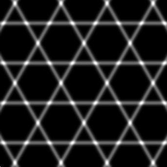
(b)

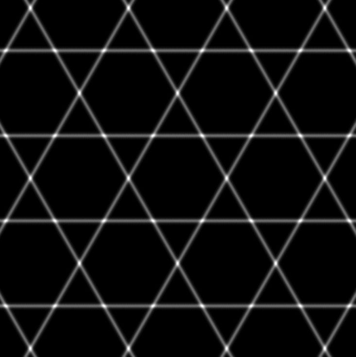
(c)

Figure 10: The Kagome potentials $V=\|V_{1}^{\nicefrac{{p}}{{2}}}+V_{3}^{\nicefrac{{p}}{{2}}}+V_{5}^{\nicefrac{{p}}{{2}}}\|_{\infty}-(V_{1}^{\nicefrac{{p}}{{2}}}+V_{3}^{\nicefrac{{p}}{{2}}}+V_{5}^{\nicefrac{{p}}{{2}}})$ for (a) $p=2$, (b) $p=10$, (c) $p=40$ with $V_{j}$ given by (4.4) for $j\in\{1,3,5\}$. Smaller values are represented by darker colors.

Remark 4.3.

Our numerical computations (see Figure 10a) show that the condition (1.8) is verified but we do not have a mathematical proof.

Remark 4.4.

We notice that the potential defined by (4.6) with

$$V_{j}(x)=\left[\cos\left(x\cdot\pi\mu_{j}+\phi_{j}\right)+2\cos\left(\frac{x\cdot\pi\mu_{j}+\phi_{j}}{3}\right)\right]^{p}\,,\quad p\in 2\mathbb{N}\,,$$

is also a kagome potential (see Figure 10). When $p$ goes to $+\infty$, we observe that the minima are very well localized at the points of $\Gamma$. This could be an advantage for verifying theoretical assumptions for an accurate semi-classical analysis of the tunneling effect between wells in the next section, but $p$ large is not experimentally reasonable.

Remark 4.5.

Considering any Bravais lattice with three points by periodicity cell, we are led to the same situation, but the kagome lattice have a much richer structure.

5 The Schrödinger magnetic operator on $L^{2}(\mathbb{R}^{2})$

5.1 The Schrödinger magnetic operator

We recall that we start from $P^{0}_{h,A,V}$ defined in (1.1). Since we have assumed $V\geq 0$, the operator is semi-bounded on $C_{0}^{\infty}(\mathbb{R}^{2})$ and there is an unique selfadjoint extension in $L^{2}(\mathbb{R}^{2})$, which can be obtained as the Friedrichs extension of $P^{0}_{h,A,V}$ (see for example [Hel13]). It can be proved that the domain of $P_{h,A,V}$ is given by

$$\mathcal{D}(P_{h,A,V})=\Big{\{}u\in L^{2}(\mathbb{R}^{2})\,;\,P_{h,A,V}\,u\in L^{2}(\mathbb{R}^{2})\Big{\}}\,.$$ (5.1)

5.2 Quantization of $\mathcal{G}$

The use of the symmetries in the case of the square, triangular and hexagonal lattices was crucial in [HS88a] and [Ker92]. In order to take advantage of the properties of the kagome lattice, we need to quantify the elements of $\mathcal{G}$, that is, to associate which each element of $\mathcal{G}$ an unitary transformation in $L^{2}(\mathbb{R}^{2})$, which respects the domain and commutes with $P_{h,A,V}$. These operators will be used later to study the low lying spectrum of $P_{h,A,V}$. We note that the quantization of the translations $T_{j}$ was introduced by Zak in [Zak64]. We also mention the work of Helffer and Sjöstrand ([HS88b], pages 147-148) who studied the case of constant magnetic field in arbitrarily dimension (see also Bellissard ([Bel87]), Cartier ([Car65]) and Zak.

Since the symmetries of the kagome lattice are dictated by those of the triangular lattice, we will use the construction of the first author in Section 1 of [Ker92]. We explain in the following the main ideas.

5.2.1 Quantization of the rotation and the translations

We now quantify the rotation $r$ and the translations $t_{j}$. We notice that for every $g\in\mathcal{G}$ the $1$-form $A-gA$ is closed and in fact it is exact. Indeed, by assumption (1.10),

$$d(A-gA)=dA-g\,dA=B-gB=0\,.$$ (5.2)

Hence, there is a real smooth function $\phi_{g}$, defined up to a constant, such that

$$A-gA=d\phi_{g}\,.$$ (5.3)

Later, we will use this freedom of choice of the constants to obtain simple commutation properties.

We may then quantize $g\in\mathcal{G}$ by the operator $T_{g}$, defined on $C^{\infty}_{0}(\mathbb{R}^{2})$ by

$$(T_{g}u)(x)=e^{\frac{i}{h}\phi_{g}(x)}\,u(g^{-1}(x))\,,$$ (5.4)

where $\phi_{g}$ is the a real function associated with $g$ by (5.3).

Lemma 5.1.

For any $g\in\mathcal{G}$, the operator $T_{g}$ is unitary on $L^{2}(\mathbb{R}^{2})$ and commutes with $P_{h,A,V}$.

Proof. For the first assertion a simple computation gives

$$T_{g}^{-1}=e^{-\frac{i}{h}g^{-1}\phi_{g}}\,g^{-1}=T_{g}^{*}\,.$$ (5.5)

We have the equality between 1-forms

$$(-ihd-A)T_{g}u = e^{i\nicefrac{{\phi_{g}}}{{h}}}\,((d\phi_{g})\,gu-ih\,g(du)-A\,(gu))\,,$$

so using (5.3) we get

$$(-ihd-A)T_{g}u = e^{i\nicefrac{{\phi_{g}}}{{h}}}\,(-ih\,g(du)-(gA)\,(gu))$$

$$= e^{i\nicefrac{{\phi_{g}}}{{h}}}\,g(-ihdu-Au)$$

$$= T_{g}(-ihd-A)u\,,$$

which gives the lemma.
∎

5.2.2 Definition of the magnetic rotation and translations

For $j=1,2,3$ we define the magnetic translations

$$T_{j}=e^{\frac{i}{h}\phi_{j}}\,t_{j}\,,$$ (5.6)

where $\phi_{j}$ is the real function associated with $t_{j}$ by (5.3) with $g=t_{j}$.

The inverse of $T_{j}$ is given by (5.5) and is also a magnetic translation. For $j=4,5,6$ we then define

$$T_{j}=T_{j+3}^{-1}\,.$$ (5.7)

We also define the magnetic rotation

$$F=e^{\frac{i}{h}f}\,r^{-1}\,,$$ (5.8)

where $f$ is the real function associated with $g=r^{-1}$ by (5.3).

Remark 5.2.

We need a convenient choice of $T_{g_{1}g_{2}}$ in order to be able to compare with $T_{g_{1}}\circ T_{g_{2}}$ (see (5.17) below). Hence, we will only use the previous construction for $r$ and $t_{j}$, $j\in\nicefrac{{\mathbb{Z}}}{{6\mathbb{Z}}}$ .

Remark 5.3.

In the case of a constant magnetic field, choosing the gauge $A(x_{1},x_{2})=\frac{B}{2}(-x_{2},x_{1})$ we have

$$f(x)=f_{0}\qquad\text{ and }\qquad\phi_{j}(x)=-\frac{B}{2}\,x\wedge(2\nu_{j})+c_{j}\,,$$

where $f_{0}$ and $c_{j}$, $j=1,2,3$, are arbitrary constants.

5.2.3 Commutation rules

We now show how a good choice of the constants appearing in the definition of $f$ and $\phi_{j}$ lead to nice commutation rules for the operators $F$ and $T_{j}$.

Proposition 5.4.

(i) The flux of $B$ through a fundamental domain $\mathcal{V}$ of $\Gamma_{\triangle}$ does not depend on the basis chosen. We write

$$\gamma=\frac{1}{h}\int_{\mathcal{V}}d\omega_{A}\,.$$

(ii) We have

$$T_{j}T_{j+1}=e^{i\gamma}T_{j+1}T_{j}\,.$$ (5.9)

(iii) There are unique $\phi_{1}$, $\phi_{2}$, $\phi_{3}$ and $f$ such that

$$F^{6} = Id_{L^{2}(\mathbb{R}^{2})}\,,$$ (5.10)

$$T_{j}F = FT_{j+1}\,,$$ (5.11)

and for these $\phi_{1}$, $\phi_{2}$ and $\phi_{3}$ we have

$$T_{j}T_{j+2}=e^{i\frac{\gamma}{2}}T_{j+1}\,.$$ (5.12)

From now on, we choose $\phi_{1}$, $\phi_{2}$, $\phi_{3}$ and $f$ in the definition of $T_{1}$, $T_{2}$, $T_{3}$ and $F$ such that (5.10)-(5.12) are satisfied.

Remark 5.5.

In the case of a constant magnetic field, choosing $A(x_{1},x_{2})=\frac{B}{2}(-x_{2},x_{1})$ we verify

$$f_{0}=c_{1}=c_{2}=c_{3}=0\,.$$

Proof of Proposition 5.4. The translations $t_{j}$ commute between them so we have

$$T_{j}T_{j+1}=e^{\frac{i}{h}\{\phi_{j}+t_{j}\phi_{j+1}-\phi_{j+1}-t_{j+1}\phi_{j}\}}T_{j+1}T_{j}\,.$$

After (5.2), the expression between the brackets here before is a constant that we note $\eta_{j}$. Using (5.3) we compute

$$(\phi_{j}-t_{j+1}\phi_{j})(x) = \int_{[x-2\nu_{j+1},x]}d\phi_{j}$$

$$= \int_{[x-2\nu_{j+1},x]}(A-t_{j}A)$$

$$= \int_{[x-2\nu_{j+1},x]}A+\int_{[x-2\nu_{j},x-2\nu_{j}-2\nu_{j+1}]}A\,,$$

where $[x,y]$ denotes the path $[0,1]\ni s\mapsto(1-s)x+sy$. Similarly,

$$(t_{j}\phi_{j+1}-\phi_{j+1})(x) = \int_{[x,x-2\nu_{j}]}A+\int_{[x-2\nu_{j}-2\nu_{j+1},x-2\nu_{j+1}]}A\,.$$

Hence, Stokes theorem yields

$$\eta_{j}=\int_{\mathcal{V}_{j,j+1}}d\omega_{A}\,,$$ (5.13)

where $\mathcal{V}_{j,j+1}$ is a cell of periodicity of the lattice generated by $2\nu_{j}$ and $2\nu_{j+1}$ with vertex $x$, $x-2\nu_{j+1}$, $x-2\nu_{j}$ and $x-2\nu_{j}-2\nu_{j+1}$. After (1.10) the magnetic field $Bdx_{1}\wedge dx_{2}$ is invariant by $r$, so the value of the $\eta_{j}$ do not depend on $j\in\nicefrac{{\mathbb{Z}}}{{6\mathbb{Z}}}$ and we have $\gamma=\eta_{1}/h$. We have proved (i) and (ii).

Since $r^{6}=id_{\mathbb{Z}^{2}}$ we have

$$F^{6}=e^{\frac{i}{h}\{f+rf+\cdots+r^{5}f\}}\,.$$ (5.14)

After (5.2) the expression between the brackets here before is a constant. Hence, choosing an appropriate constant in the definition of $f$ we obtain (5.10).

Using (4.1) and (5.7) we have

$$T_{1}F = e^{\frac{i}{h}\{\phi_{1}+t_{1}f-f-r^{-1}\phi_{2}\}}FT_{2}\,,$$

$$T_{2}F = e^{\frac{i}{h}\{\phi_{2}+t_{2}f-f-r^{-1}\phi_{3}\}}FT_{3}\,,$$

$$T_{3}F = e^{\frac{i}{h}\{\phi_{3}+t_{3}f-f+t_{3}r^{-1}\phi_{1}\}}FT_{4}\,.$$

As before, using (5.2) the expressions between the brackets in the previous equalities are constants. If we respectively add $a_{1}$, $a_{2}$ and $a_{3}$ to $\phi_{1}$, $\phi_{2}$ and $\phi_{3}$, the expressions between the brackets are respectively modified by $a_{1}-a_{2}$, $a_{2}-a_{3}$ and $a_{1}+a_{3}$. Hence, there exist $a_{1}$, $a_{2}$ and $a_{3}$ such that (5.11) is satisfied for $j=1,2,3$. Since $T_{j+3}=T_{j}^{-1}$, (5.11) also holds for $j=4,5,6$.

Again, we have that $\{\phi_{j}+t_{j}\phi_{j+2}-\phi_{j+1}\}$ is a constant that we call $c$, so

$$T_{j}T_{j+2}=e^{i\frac{c}{h}}\,T_{j+1}\,.$$ (5.15)

Using the conjugation by $F$ and (5.11), we then obtain $e^{i\frac{c}{h}}\,T_{j+2}=T_{j+1}T_{j}^{-1}$, which gives

$$T_{j}T_{j+2}=e^{i\frac{2c}{h}}T_{j+2}T_{j}\,.$$ (5.16)

The proof of (5.9) also applies when taking $T_{j}$ and $T_{j+2}$ instead of $T_{j}$ and $T_{j+1}$, so we have $T_{j}T_{j+2}=e^{i\frac{\eta_{1}}{h}}T_{j+2}T_{j}$. Thus, $2c/h\equiv\eta_{1}/h\,\,[2\pi]$, which gives $(c-\eta_{1}/2)/h\in\pi\mathbb{Z}$. Since $c$ and $\eta_{1}$ do not depend on $h$, we derive that necessarily $c=\eta_{1}/2$, which yields (5.12). We have proved (iii).
∎

Now, for $\alpha\in\mathbb{Z}^{2}$ we define the magnetic translations

$$T^{\alpha}=e^{-i\frac{\gamma}{2}\alpha_{1}\alpha_{2}}\,T_{1}^{\alpha_{1}}T_{2}^{\alpha_{2}}\,.$$ (5.17)

We obtain the following relations (see also [Ker92], pages 15-16):

Proposition 5.6.

For every $\alpha,\beta\in\mathbb{Z}^{2}$,

$$(T^{\alpha})^{-1} = T^{-\alpha}_{,},$$ (5.18)

$$T^{\alpha}T^{\beta} = e^{i\frac{\gamma}{2}\alpha\wedge\beta}\,T^{\alpha+\beta}\,,$$ (5.19)

$$FT^{\alpha} = T^{\kappa^{-1}(\alpha)}F\,.$$ (5.20)

Proof of Proposition 5.6. Using (5.9) we have $T_{1}^{\alpha_{1}}T_{2}^{\alpha_{2}}=e^{i\alpha_{1}\alpha_{2}\gamma}T_{2}^{\alpha_{2}}T_{1}^{\alpha_{1}}$, which gives

$$(T^{\alpha})^{-1} = e^{\frac{i\gamma}{2}\alpha_{1}\alpha_{2}}\,\,T_{2}^{-\alpha_{2}}T_{1}^{-\alpha_{1}}$$

$$= e^{\frac{i\gamma}{2}(\alpha_{1}\alpha_{2}-2\alpha_{1}\alpha_{2})}\,\,T_{1}^{-\alpha_{1}}T_{2}^{-\alpha_{2}}$$

$$= T^{-\alpha}\,$$

and

$$T^{\alpha}T^{\beta} = e^{-\frac{i\gamma}{2}(\alpha_{1}\alpha_{2}+\beta_{1}\beta_{2})}\,\,T_{1}^{\alpha_{1}}T_{2}^{\alpha_{2}}T_{1}^{\beta_{1}}T_{2}^{\beta_{2}}$$

$$= e^{-\frac{i\gamma}{2}(\alpha_{1}\alpha_{2}+\beta_{1}\beta_{2}+2\alpha_{2}\beta_{1})}\,\,T_{1}^{\alpha_{1}+\beta_{1}}T_{2}^{\alpha_{2}+\beta_{2}}$$

$$= e^{\frac{i\gamma}{2}(\alpha\wedge\beta)}\,\,T^{\alpha+\beta}\,.$$

Using (5.12) we have $T_{1}^{\alpha_{1}}T_{3}^{\alpha_{1}}=e^{\frac{i\gamma}{2}\alpha_{1}^{2}}T_{2}^{\alpha_{1}}$. Hence, after (5.7) and (5.11) we get

$$FT^{\alpha} = e^{-\frac{i\gamma}{2}\alpha_{1}\alpha_{2}}\,\,FT_{1}^{\alpha_{1}}T_{2}^{\alpha_{2}}$$

$$= e^{-\frac{i\gamma}{2}\alpha_{1}\alpha_{2}}\,\,T_{3}^{-\alpha_{1}}T_{1}^{\alpha_{2}}F$$

$$= e^{-\frac{i\gamma}{2}(\alpha_{1}\alpha_{2}+\alpha_{1}^{2})}\,\,T_{2}^{-\alpha_{1}}T_{1}^{\alpha_{1}+\alpha_{2}}F$$

$$= e^{-\frac{i\gamma}{2}(\alpha_{1}+\alpha_{2})(-\alpha_{1})}\,\,T_{1}^{\alpha_{1}+\alpha_{2}}T_{2}^{-\alpha_{1}}F$$

$$= T^{k^{-1}(\alpha)}F\,.$$

∎

5.3 The harmonic approximation

Here we recall a result from [HS87] about the semiclassical analysis of the bottom of the spectrum of a Schrödinger operator with magnetic field in the case when the electric potential $V$ has a unique non degenerate well at a point $m$.

The theory of the harmonic approximation was initially introduced for a Schrödinger operator without magnetic field in [HS84] and [Sim83] and can be extended to the magnetic case. More precisely, the harmonic approximation consists in replacing the potential $V$ by its quadratic approximation at $m$ and the magnetic field by its value at $m$, that is the magnetic potential by its linear part at $m$. This reads:

$$P_{har,h,B}=h^{2}D_{x_{1}}^{2}+(hD_{x_{2}}-Bx_{1})^{2}+\frac{1}{2}\langle{\rm Hess}\,V(m)\,x,x\rangle\,$$ (5.21)

with $B=B(m)$. The following result is classical and can for example be found in [Hel09]:

Proposition 5.7.

Assume that ${\rm Hess}\,V(m)>0$. The spectrum of the operator $P_{har,h,B}$ defined in (5.21) is discrete. The first eigenvalue is simple and given by

$$\lambda_{har,h,B}=h\sqrt{\lambda^{2}_{1,0}+B^{2}}\,,$$

where $\lambda_{1,0}=(\sqrt{\lambda_{1}}+\sqrt{\lambda_{2}})/\sqrt{2}$ is the first eigenvalue of $P_{har,1,0}$ and $\lambda_{1}$,$\lambda_{2}$ are the eigenvalues of ${\rm Hess}\,V(m)$.

Proof. Possibly after changes of coordinates and gauge, $P_{har,h,B}$ is written

$$P_{har,h,B}=h^{2}D_{x_{1}}^{2}+(hD_{x_{2}}-Bx_{1})^{2}+\frac{\lambda_{1}}{2}x_{1}^{2}+\frac{\lambda_{2}}{2}x_{2}^{2}\,.$$

A partial Fourier transform in the second variable leads to the operator

$$h^{2}D_{x_{1}}^{2}+(h\xi_{2}-Bx_{1})^{2}+\frac{\lambda_{1}}{2}x_{1}^{2}+\frac{\lambda_{2}}{2}D_{\xi_{2}}^{2}\,,$$

which after the dilation $\displaystyle y_{2}=\frac{h\xi_{2}}{\sqrt{\lambda_{2}/2}}$ becomes

$$h^{2}D_{x_{1}}^{2}+h^{2}D_{y_{2}}^{2}+(\sqrt{\frac{\lambda_{2}}{2}}y_{2}-Bx_{1})^{2}+\frac{\lambda_{1}}{2}x_{1}^{2}\,.$$

A new change of coordinates leads to the sum of the two harmonic oscillators $h^{2}D_{z_{j}}^{2}+\mu_{j}z_{j}^{2}$, $j=1$, $2$, where $\mu_{1}$, $\mu_{2}$ are the eigenvalues of the quadratic form $(\sqrt{\lambda_{1}/2}y_{2}-Bx_{1})^{2}+\frac{\lambda_{1}}{2}x_{1}^{2}$. These oscillators have discrete spectrum and their lowest eigenvalues are $h\sqrt{\mu_{j}}$. A straightforward computation gives

$$(\sqrt{\mu_{1}}+\sqrt{\mu_{2}})^{2}=B^{2}+\lambda_{1,0}^{2}\,.$$

∎

A result of [HS87] allows then to estimate the first eigenvalue of a single well Schrödinger operator using the harmonic approximation. We also refer to [CFKS87], §11 for other results in this spirit.

Proposition 5.8.

Consider a vector field $\tilde{A}=(\tilde{A}_{1},\tilde{A}_{2})\in C^{\infty}(\mathbb{R}^{2})$ and a real nonnegative potential $\tilde{V}\in C^{\infty}(\mathbb{R}^{2})$ with a unique non degenerate minimum at a point $m\in\mathbb{R}^{2}$. The smallest eigenvalue $\lambda_{h,B}$ of the magnetic Schrödinger operator

$$P_{h,\tilde{A},\tilde{V}}=(hD_{x_{1}}-\tilde{A}_{1}(x))^{2}+(hD_{x_{2}}-\tilde{A}_{2}(x))^{2}+\tilde{V}(x)$$ (5.22)

is simple and satisfies

$$|\lambda_{h,B}-h\lambda_{har,1,B}|\leq Ch^{\nicefrac{{3}}{{2}}}\,.$$

Moreover, there exists $\epsilon_{0}>0$ such that $\sigma(P_{h,\tilde{A},\tilde{V}})\cap[0,h(\lambda_{har,1,B}+\epsilon_{0})]=\{\lambda_{h,B}\}$.

Remark 5.9.

In the case of a weak constant magnetic field $B=hB_{0}$, the harmonic approximation has no magnetic contribution and we have

$$|\lambda_{h,B}-h\lambda_{har,1,0}|\leq Ch^{\nicefrac{{3}}{{2}}}\,.$$

5.4 Agmon distance

Consider the Agmon metric $V\,dx^{2}$. For a piecewise $C^{1}$ curve $\eta$, we can define its length $|\eta|$ in this metric, and for $x,y\in\mathbb{R}^{2}$ we define the Agmon distance $d_{V}(x,y)$ as the $\inf|\eta|$ over all piecewise $C^{1}$ curves $\eta$ joining $x$ to $y$. This distance may be degenerate in the sense that $d_{V}(x,y)=0$ for $x\neq y$, but it satisfies standard properties such as

$$d_{V}(x,y)=d_{V}(y,x)\quad\text{ and }\quad d_{V}(x,z)\leq d_{V}(x,y)+d_{V}(y,z)\,.$$

In the following, for $\varphi\in L^{2}(\mathbb{R}^{2})$ and $y\in\mathbb{R}^{2}$ we will use the notation

$$\varphi=\mathcal{O}_{\epsilon}\left(e^{\frac{-d_{V}(\cdot,y)(1-\epsilon)+\epsilon}{h}}\right)\,,$$

which means that for every $\epsilon>0$, there exists $h_{\epsilon}>0$ and $C_{\epsilon}$ such that

$$\left\|e^{\frac{d_{V}(\cdot,y)(1-\epsilon)}{h}}\varphi(\cdot)\right\|_{L^{2}(\mathbb{R}^{2})}\leq C_{\epsilon}e^{\frac{\epsilon}{h}}$$

for $h\in(0,h_{\epsilon})$. Here $d_{V}(\cdot,m)$ is the Agmon distance to the point $m$. We refer to [DS99], §6 for details on Agmon estimates.

5.5 Construction of a basis of the space attached to the low lying spectrum of $P_{h,A,V}$

We now explain Carlsson’s construction of an orthonormal basis of the spectral space attached to the low lying spectrum of $P_{h,A,V}$ and prove Theorem 1.3. The approach of Carlsson is quite general (no assumption of periodicity is needed) but he does not consider the case with magnetic field. Nevertheless, the theory is simpler in the periodic case and it was shown in Section 9 of [HS88a] how to generalize this result with the help of [HS87].

We follow the method of “filling the wells” to obtain a basis of the spectral space attached to the low lying spectrum of $P_{h,A,V}$. In our setting (see (1.8)), the wells correspond to the points of the kagome lattice. The method consists then in associating with each $m\in\Gamma$, the Schrödinger operator $P_{m}$ given in (1.13), which is obtained by filling all the other wells. Then, we get the desired basis considering the space spanned by the ground states of the $P_{m}$. Moreover, this basis respects the action of the magnetic operators, which lead to properties (1.18) and (1.19).

Proof of Theorem 1.3. (Step 1) Consider the operators $P_{m}$ defined in (1.13). We have seen in Proposition 4.1 that for all $m,n\in\Gamma$ there is $g\in\mathcal{G}$ such that $g(m)=n$. Considering the associated $T_{g}$ defined in (5.5), all the operators $P_{m}$ are unitary equivalent.

A result of Persson ([Per60]) gives that $\sigma(P_{m})$ is discrete in the interval $[0,b]$ where $b$ is defined in (1.14). Each operator $P_{m}$ is a Schrödinger operator with electric potential $V+V_{m}$. Using Hypothesis 1.1, $V+V_{m}$ has a unique non degenerate minimum, so Proposition 5.8 applies to $P_{m}$. The first eigenvalue $\lambda_{h,B}$ of $P_{m}$ is simple and there exists $\epsilon_{0}>0$ such that $\sigma(P_{m})\cap I(h)=\{\lambda_{h,B}\}$, where $I(h)=[0,h(\lambda_{har,1,B(m)}+\epsilon_{0})]$.

(Step 2) Consider $m_{1}=m_{(0,0),1}$ and let $\varphi_{1}$ be an eigenfunction of $P_{m_{1}}$ with eigenvalue $\lambda(h)$ such that

$$\|\varphi_{1}\|_{L^{2}(\mathbb{R}^{2})}=1\quad\text{ and }\quad\varphi_{1}(m_{1})\text{ is real.}$$ (5.23)

For $\ell=1,3,5$ we define

$$\varphi_{\ell}=F^{1-\ell}\varphi_{1}\,,$$ (5.24)

and for every $m_{\alpha,\ell}\in\Gamma$ we define an eigenfunction of $P_{m_{\alpha,\ell}}$ with eigenvalue $\lambda(h)$, by

$$\varphi_{\tilde{m}_{\alpha,\ell}}=e^{-i\frac{\gamma}{2}\alpha\wedge\tilde{\nu}_{\ell}}\,T^{\alpha}\varphi_{\ell}\,.$$ (5.25)

Defining $r_{\tilde{m}}=(P-\lambda(h))\varphi_{\tilde{m}}$, we have the Agmon estimates

$$\varphi_{\tilde{m}},r_{\tilde{m}},\nabla_{A}\varphi_{\tilde{m}},\nabla_{A}r_{\tilde{m}}=\mathcal{O}_{\epsilon}\left(e^{\frac{-d_{V}(x,m)(1-\epsilon)+\epsilon}{h}}\right)\,,$$ (5.26)

where $\nabla_{A}=(hD_{x_{j}}-A_{j}(x))_{j=1,2}$. Moreover,

$$\text{supp}\,r_{\tilde{m}}\subset\bigcup_{n\in\Gamma\setminus\{m\}}B(n,\delta)\,.$$ (5.27)

We also observe by the harmonic approximation that

$$\varphi_{1}(\tilde{m}_{1})=h^{-\nicefrac{{1}}{{2}}}c_{har}+\mathcal{O}(1)\,.$$ (5.28)

We now give the action of the magnetic operators over the eigenfunctions $\varphi_{\tilde{m}}$. The proof of the following Proposition is given at the end of this section.

Proposition 5.10.

For every $h>0$ there exist $c\in\{-1,1\}$ such that for all $m\in\Gamma$ and $\beta\in\mathbb{Z}^{2}$ we have

$$T^{\beta}\varphi_{\tilde{m}} = e^{i\frac{\gamma}{2}\beta\wedge\tilde{m}}\,\varphi_{\tilde{m}+\beta}\,,$$ (5.29)

$$F\varphi_{\tilde{m}} = c\,\varphi_{\kappa^{-1}(\tilde{m})}\,.$$ (5.30)

(Step 3) We may now state Carlsson’s result. Let $\Sigma$ be the spectral space associated with $I(h)$ and $\Pi$ the orthogonal projection over $\Sigma$. We define the projections

$$v_{\tilde{m}}=\Pi\,\varphi_{\tilde{m}}\,,\qquad{m}\in\Gamma\,.$$ (5.31)

By estimates (5.26) and (5.27), for every $\epsilon>0$ we can choose $\delta>0$ in the definition of $P_{m}$ in (1.13) such that

$$|\left<v_{\tilde{m}},v_{\tilde{n}}\right>| \leq \exp\left(-\frac{(1-\epsilon)d_{V}(m,n)}{h}\right)\,,$$

$$|\left<v_{\tilde{m}},v_{\tilde{m}}\right>-1| \leq \exp\left(-\frac{(2S-\epsilon)}{h}\right)$$

for $h\in(0,h(\epsilon))$. We denote $D$ the matrix given by $D_{\tilde{m},\tilde{n}}=\left<v_{\tilde{n}},v_{\tilde{m}}\right>$ and we define the functions

$$e_{\tilde{m}}=\sum_{\tilde{m}\in\tilde{\Gamma}}v_{\tilde{n}}(D^{-1/2})_{\tilde{m},\tilde{n}}\,.$$ (5.32)

The functions $e_{\tilde{m}}$ form an orthonormal basis of $\Sigma$.
Let $W_{\gamma}$ be the matrix of $P_{h,A,V}|\Sigma$ in this basis and put

$$(\tilde{W})_{\gamma,\tilde{m},\tilde{n}}=\left<r_{\tilde{n}},\varphi_{\tilde{m}}\right>\,.$$

After Carlsson’s theorem, for every $\epsilon>0$ we can choose $\delta$ in the definition of $\chi$ in Step 1 such that for $h\in(0,h(\epsilon))$

$$\left|\left(W_{\gamma}\right)_{\tilde{m},\tilde{n}}-\tilde{W}_{\gamma,\tilde{m},\tilde{n}}\right|\leq\exp\left(-\frac{(1-\epsilon)\,d^{(2)}_{V}(m,n)}{h}\right)$$ (5.33)

where

$$d^{(2)}_{V}(n,m)=\min\{d_{V}(n,p)+d_{V}(p,m);\,p\in\Gamma,\,p\not=n,\,p\not=m\}.$$

This proves (1.20) and (1.21) in Theorem 1.3.

Moreover, the following proposition (which proof is given at the end of this section), proves that the orthonormalization process preserves the action of the magnetic operators.

Proposition 5.11.

For every $m\in\Gamma$ and $\beta\in\mathbb{Z}^{2}$ we have

$$T^{\beta}e_{\tilde{m}} = e^{i\frac{\gamma}{2}\beta\wedge\tilde{m}}\,e_{\tilde{m}+\beta}\,,$$ (5.34)

$$Fe_{\tilde{m}} = c\,e_{k^{-1}(\tilde{m})}\,,$$ (5.35)

where $c\in\{-1,1\}$ is defined in Proposition 5.10.

Finally, properties (1.18) and (1.19) in Theorem 1.3 follow from Lemma 5.1, together with (5.34) and (5.35).
∎

We end this section with the proofs of Propositions 5.10 and Proposition 5.11.

Proof of Proposition 5.10. Let $m=m_{\alpha,\ell}$. For the first relation, using (5.19) we have

$$T^{\beta}\varphi_{\tilde{m}} = e^{-i\frac{\gamma}{2}\alpha\wedge\tilde{\nu}_{\ell}}\,T^{\beta}T^{\alpha}\varphi_{\ell}$$

$$= e^{-i\frac{\gamma}{2}\left(\alpha\wedge\tilde{\nu}_{\ell}-\beta\wedge\alpha\right)}\,T^{\alpha+\beta}\varphi_{\ell}$$

$$= e^{i\frac{\gamma}{2}\beta\wedge\tilde{m}}\,e^{-i\frac{\gamma}{2}(\alpha+\beta)\wedge\tilde{\nu}_{\ell}}\,T^{\alpha+\beta}\varphi_{\ell}$$

$$= e^{i\frac{\gamma}{2}\beta\wedge\tilde{m}}\,\varphi_{\tilde{m}+\beta}\,.$$

After (1.4) and (4.2) we have

$$\kappa^{-1}(m_{\alpha,\ell}) = \kappa^{-1}(\alpha)+\frac{1}{2}\kappa^{\ell-2}(1,0)$$

$$= \kappa^{-1}(\alpha+\kappa^{\ell-1}(1,0))+\frac{1}{2}\kappa^{\ell+1}(1,0)$$

$$= \tilde{m}_{\kappa^{-1}(\alpha+\kappa^{\ell-1}(1,0)),\ell+2}$$

and

$$\kappa^{-1}(\alpha+\kappa^{\ell-1}(1,0))\wedge\tilde{\nu}_{\ell+2}=-\kappa^{-1}(\alpha)\wedge\frac{1}{2}\kappa^{\ell-2}(1,0)\,,$$

so we have to prove that

$$F\varphi_{\tilde{m}}=c\,e^{i\frac{\gamma}{2}\kappa^{-1}(\alpha)\wedge\frac{1}{2}\kappa^{\ell-2}(1,0)}T^{\kappa^{-1}(\alpha+\kappa^{\ell-1}(1,0))}\,\varphi_{\ell+2}$$ (5.36)

for some $c\in\{-1,1\}$.

Using (4.1) we have $t_{1}r^{3}V_{m_{1}}=V_{m_{1}}$ so $T_{1}F^{3}$ commutes with the multiplication by $V_{m_{1}}$. Lemma 5.1 yields then that $T_{1}F^{3}$ commutes with $P_{m_{1}}$. Hence, since $\lambda(h)$ is a simple eigenvalue, there is a complex number $c$, such that $|c|=1$ and

$$T_{1}F^{3}\varphi_{1}=c\,\varphi_{1}\,.$$ (5.37)

Moreover, (5.10) and (5.11) yield $(T_{1}F^{3})^{2}=Id_{L^{2}(\mathbb{R}^{2})}$, so $c^{2}=1$. Using (5.20) and (5.37) we have

$$F\varphi_{1}=c\,F^{4}T^{-1}_{1}\varphi_{1}=c\,T^{\kappa^{-4}(-1,0)}F^{4}\varphi_{1}=c\,T^{\kappa^{-1}(1,0)}F^{-2}\varphi_{1}\,.$$

Considering (1.4), (4.2), (5.19) and (5.20), the previous equality gives

$$F\varphi_{\tilde{m}} = e^{-i\frac{\gamma}{2}\alpha\wedge\tilde{\nu}_{\ell}}\,T^{\kappa^{-1}(\alpha)}F^{1-\ell}F\varphi_{1}$$

$$= c\,e^{-i\frac{\gamma}{2}\alpha\wedge\tilde{\nu}_{\ell}}\,T^{\kappa^{-1}(\alpha)}F^{1-\ell}T^{\kappa^{-1}(1,0)}F^{-2}\varphi_{1}$$

$$= c\,e^{-i\frac{\gamma}{2}\alpha\wedge\tilde{\nu}_{\ell}}\,T^{\kappa^{-1}(\alpha)}T^{\kappa^{\ell-2}(1,0)}_{1}F^{1-(\ell+2)}\varphi_{1}$$

$$= c\,e^{-i\frac{\gamma}{2}\kappa^{-1}(\alpha)\wedge\left(\frac{1}{2}\kappa^{\ell-2}(1,0)-\kappa^{\ell-2}(1,0)\right)}\,T^{\kappa^{-1}(\alpha+\kappa^{\ell}(1,-1))}\,\varphi_{\ell+2}\,,$$

which yields (5.36) and ends the proof.
∎

Proof of Proposition 5.11. After Lemma 5.1, $T^{\beta}$ commutes with $P_{h,A,V}$, so also with $\Pi$ using the functional calculus of $P_{h,A,V}$. Then, using (5.29), (5.31) and (5.32) we get

$$T^{\beta}e_{\tilde{m}} = \sum_{\tilde{n}}T^{\beta}v_{\tilde{n}}\,(D^{-1/2})_{\tilde{m},\tilde{n}}$$

$$= \sum_{\tilde{n}}e^{i\frac{\gamma}{2}\beta\wedge\tilde{n}}\,v_{\tilde{n}+\beta}(D^{-1/2})_{\tilde{m},\tilde{n}}$$

$$= e^{i\frac{\gamma}{2}\beta\wedge\tilde{m}}\,\sum_{\tilde{n}}v_{\tilde{n}+\beta}\,e^{-i\frac{\gamma}{2}\beta\wedge\tilde{m}}\,(D^{-1/2})_{\tilde{m},\tilde{n}}\,e^{i\frac{\gamma}{2}\beta\wedge\tilde{n}}\,.$$

Since $T^{\beta}$ is unitary, (5.29) yields

$$\hat{D}_{\tilde{m},\tilde{n}}:=\left<v_{\tilde{n}+\beta},v_{\tilde{m}+\beta}\right>=e^{-i\frac{\gamma}{2}\beta\wedge\tilde{m}}\,D_{\tilde{m},\tilde{n}}e^{i\frac{\gamma}{2}\beta\wedge\tilde{n}}\,.$$

Considering the diagonal matrix $A_{\tilde{m},\tilde{m}}=e^{-i\frac{\gamma}{2}\beta\wedge\tilde{m}}$, we note that

$$\left((ADA^{-1})^{-1/2}\right)_{\tilde{m},\tilde{n}}=e^{-i\frac{\gamma}{2}\beta\wedge\tilde{m}}\,(D^{-1/2})_{\tilde{m},\tilde{n}}\,e^{i\frac{\gamma}{2}\beta\wedge\tilde{n}}\,,$$

so (5.5) becomes

$$T^{\beta}e_{\tilde{m}} = e^{i\frac{\gamma}{2}\beta\wedge\tilde{m}}\,\sum_{\tilde{n}}v_{\tilde{n}+\beta}(\hat{D}^{-1/2})_{\tilde{m},\tilde{n}}\,.$$

We get (5.34) noting that the sum in the right hand side of the previous equality is the $\tilde{m}+\beta$ vector in the orthonormalization of $\{v_{\tilde{n}}\}$.

Similarly, using (5.30) we find

$$Fe_{\tilde{m}}=c\,\sum_{\tilde{n}}v_{\kappa^{-1}(\tilde{n})}(D^{-1/2})_{\tilde{m},\tilde{n}}\,,$$ (5.39)

and since the magnetic rotation is a unitary operator, we have $D=\tilde{D}$ where

$$\tilde{D}_{\tilde{m},\tilde{n}}=\left<v_{\kappa^{-1}(\tilde{n})},v_{\kappa^{-1}(\tilde{m})}\right>\,.$$ (5.40)

Hence,

$$Fe_{\tilde{m}} = c\,\sum_{\tilde{n}}v_{\kappa^{-1}(\tilde{n})}(\tilde{D}^{-1/2})_{\tilde{m},\tilde{n}}\,.$$

We get (5.35) reasoning as before.
∎

6 The reduced models

6.1 Introduction

In this section we obtain and study the reduced models associated with the low lying spectrum of $P_{h,A,V}$. First, under Hypothesis 1.4 and in the case of a weak and constant magnetic field, we estimate the coefficients of $W_{\gamma}$ corresponding to the nearest neighbours for the Agmon distance. Then, by only keeping these terms, we construct the operators $Q_{\gamma,\omega}$ and $P^{kay}_{\gamma,\omega}$ and prove Theorems 1.5 and 1.6. We then look at the case of rational values of the renormalized flux and reduce the operator $W_{\gamma}$ to a family of hermitian matrices. We end this article by proving the symmetries of the spectrum and the existence of eigenvalues and flat bands.

6.2 The nearest neighbors and the tunneling effect

As in [HS88a] and [Ker92], we implement here the results of [HS87] about the tunneling effect to estimate the coefficients of $W_{\gamma}$ corresponding to the nearest neighbours for the Agmon distance.

For any $\alpha\in\mathbb{Z}^{2}$ we want to identify in $W_{\gamma}$ the main terms corresponding to the interactions between the nearest wells for the Agmon distance to the triple $\{m_{\alpha,1},m_{\alpha,3},m_{\alpha,5}\}$. After Hypothesis 1.4 A, the nearest neighbours for the Agmon distance of a point $m_{\alpha,j}\in\Gamma$ are (see Figure 1):

$$m_{(\alpha+2\tilde{\nu}_{j}),j-2}\,,m_{(\alpha-2\tilde{\nu}_{j-2}),j-2}\,,m_{(\alpha+2\tilde{\nu}_{j}),j+2}\text{ and }m_{(\alpha-2\tilde{\nu}_{j+2}),j+2}\,.\quad$$ (6.1)

Proof of Theorems 1.5 and 1.6. (Step 1) First, we notice that the term $e^{-\frac{i\gamma}{2}\alpha\wedge\tilde{\nu}_{\ell}}$ from the definition of the eigenfunctions in (5.25) give the nice relations of Proposition 5.11, but leads to the matrix $W_{\gamma}$ which does not satisfy the hypotheses of Theorem 2.1. To solve this, we introduce the new basis $\{f_{\tilde{m}}\}_{m\in\Gamma}$

$$f_{\tilde{m}_{\alpha,j}}=e^{i\frac{\gamma}{2}\alpha\wedge\tilde{\nu}_{j}}e_{\tilde{m}_{\alpha,j}}\,.$$ (6.2)

such that

$$T^{\beta}f_{\tilde{m}_{\alpha,j}}=e^{i\frac{\gamma}{2}\beta\wedge\alpha}f_{\tilde{m}_{\alpha+\beta,j}}\,.$$ (6.3)

Let $M$ be the matrix of $P_{h,A,V}-\lambda(h)\,I$ in this new basis. We denote by $M_{\alpha,\beta}^{j,k}$ the coefficients of $M$ in $\mathbb{C}$ and by $M_{\alpha,\beta}$ the blocks in $M_{3}(\mathbb{C})$ (i.e. $\left(M_{\alpha,\beta}\right)^{j,k}=M_{\alpha,\beta}^{j,k}$). The matrix $M$ is obtained by conjugation by the diagonal matrix $A$ acting on $\ell^{2}(\mathbb{Z}^{2};\mathbb{C}^{3})$ by

$$A_{\alpha,\alpha}^{jj}=e^{i\frac{\gamma}{2}\alpha\wedge\tilde{\nu}_{j}}\,,$$

so we obtain

$$\ M_{\alpha,\beta}^{j,k}=e^{-i\frac{\gamma}{2}(\alpha\wedge\tilde{\nu}_{j}-\beta\wedge\tilde{\nu}_{k})}W_{\tilde{m}_{\alpha,j},\tilde{m}_{\beta,k}}\,.$$ (6.4)

The matrix $M$ thus inherits the properties of $W_{\gamma}$. Indeed, (1.18) and (1.19) yield

$$M_{\alpha,\beta} = e^{i\frac{\gamma}{2}(\alpha-\beta)\wedge\delta}M_{\alpha+\delta,\beta+\delta}\,,$$ (6.5)

$$M_{\alpha,\beta}^{j,k} = e^{i\frac{\gamma}{2}(\kappa^{-1}(\alpha)\wedge\tilde{\nu}_{j+2}-\kappa^{-1}(\beta)\wedge\tilde{\nu}_{k+2})}M^{j+2,k+2}_{\kappa^{-1}(\alpha)+\kappa^{j-2}(1,0),\beta+\kappa^{k-2}(1,0)}$$ (6.6)

for $\alpha$, $\beta$, $\delta\in\mathbb{Z}^{2}$ and $j$,$k\in\{1,3,5\}$, where $\kappa$ is defined in (1.5).

Relation (6.5) implies

$$M_{\alpha,\beta}=e^{-i\frac{\gamma}{2}\alpha\wedge\beta}M_{\alpha-\beta,0}\,,$$

which allows us to apply Theorem 2.1. Hence, we define the operator

$$Q_{\gamma}=\sum_{\beta\in\mathbb{Z}^{2}}e^{i\frac{\gamma}{2}\beta_{1}\beta_{2}}\,M_{\beta,0}\,\tau_{1}^{\beta_{1}}\tau_{2}^{\beta_{2}}$$ (6.7)

on $\ell^{2}(\mathbb{Z}^{2};\mathbb{C}^{3})$ and the symbol

$$p(x,\xi,\gamma)=\sum_{\beta\in\mathbb{Z}^{2}}M_{\beta,0}\,e^{i(\beta_{1}x+\beta_{2}\xi)}\,,$$ (6.8)

and obtain that $W_{\gamma}$ and $Q_{\gamma}$ are unitary equivalent, and that the Weyl quantization $P_{\gamma}$ of $p(x,\xi,\gamma)$ and $W_{\gamma}$ have the same spectrum.

(Step 2) We now compute the relations between the terms of $M_{\beta,0}$ corresponding to the interactions between the nearest wells of $V$. We have to consider 12 terms, which correspond to the neighbours given in (6.1) for $\alpha=(0,0)$ and $j=1,3,5$. Relations (6.4) and (6.5) yield

$$M_{(-1,0),(0,0)}^{1,3}=e^{i\frac{\gamma}{4}}\,W_{\tilde{m}_{(0,0),1},\tilde{m}_{(1,0),3}}\,.$$ (6.9)

Combining (6.6) and (6.5) we find $M_{(-1,0),(0,0)}^{1,3}=M_{(0,-1),(0,0)}^{3,5}$. Hence, using (6.6) twice,

$$M_{(-1,1),(0,0)}^{1,3}=M_{(1,0),(0,0)}^{5,1}=M_{(0,-1),(0,0)}^{3,5}=M_{(1,-1),(0,0)}^{3,5}=M_{(0,1),(0,0)}^{5,1}=M_{(-1,0),(0,0)}^{1,3}\,.$$

By the self-adjointness of $P_{h,A,V}$, the other six terms equal the complex conjugate of $M_{(-1,0),(0,0)}^{1,3}$.

(Step 3) We now estimate $M_{(-1,0),(0,0)}^{1,3}$ when $A$ is given by (1.22) and $V$ satisfies Hypothesis 1.4. First,

$$\gamma=B_{0}\,(2\nu_{1})\wedge(2\nu_{2})=2\sqrt{3}B_{0}\,.$$ (6.10)

We compute explicitly the value of the phases of the magnetic translations and rotation. Remarks 5.3 and 5.5, together with (6.10), give that for any $\alpha\in\mathbb{Z}^{2}$ and $\varphi\in L^{2}(\mathbb{R}^{2})$

$$(T^{\alpha}\varphi)(x)=e^{-i\frac{B_{0}}{2}\,x\wedge\left(2\alpha_{1}\nu_{1}+2\alpha_{2}\nu_{2}\right)}\,\varphi\left(\tau^{-\alpha}(x)\right)\quad\text{ and }\quad(F\varphi)(x)=\varphi(r(x))\,.$$ (6.11)

The results in Section 3 of [HS87] give an asymptotic estimate for $(W_{\gamma})_{\tilde{m}_{(0,0),1},\tilde{m}_{(1,0),3}}$. In order to apply the results there, we first need to verify that the values of the functions $\varphi_{\tilde{m}_{(0,0),1}}$ and $\varphi_{\tilde{m}_{(1,0),3}}$ at the bottom of their respective wells are real. The value of $\varphi_{\tilde{m}_{(0,0),1}}(m_{(0,0),1})=\varphi_{1}(\nu_{1})$ has been chosen real in (5.23). The definition of $\varphi_{\tilde{m}}$ in (5.25) and $m_{(1,0),3}=\nu_{1}+\nu_{2}$, together with (6.10) and (6.11), give

$$\varphi_{\tilde{m}_{(1,0),3}}(m_{(1,0),3}) = e^{-i\frac{\gamma}{2}\,2\tilde{\nu}_{1}\wedge\tilde{\nu}_{3}}\,\left(T_{1}F^{-2}\varphi_{1}\right)(\nu_{2})$$

$$= e^{-i\frac{B_{0}}{4}\,(2\nu_{1})\wedge(2\nu_{2})}\,e^{-i\frac{B_{0}}{2}\,\nu_{2}\wedge 2\nu_{1}}\,\varphi_{1}(r^{-2}(\nu_{3}))$$

$$= \varphi_{1}(\nu_{1})\,,$$

so $\varphi_{\tilde{m}_{(1,0),3}}(m_{(1,0),3})$ is also real.

The results in [HS87] are given for a magnetic potential $A_{t}=tA$, with the condition (see (2.40) therein) $|t|=\mathcal{O}(h^{\nicefrac{{1}}{{2}}}(-\ln h)^{\nicefrac{{1}}{{2}}})$. Our setting satisfies this requirement with $t=h$. By Proposition 3.12, Remark 3.17 and Lemma 3.15 in [HS87] and assuming Hypothesis 1.4 we get

$$(W_{\gamma})_{\tilde{m}_{(0,0),1},\tilde{m}_{(1,0),3}}=h^{\nicefrac{{1}}{{2}}}\,b(h)\,e^{-\frac{S(h)}{h}}\,,$$

where

$$\begin{array}[]{rl}|b(h)|=b_{0}+\mathcal{O}(h)\,,&\text{Re}(S(h))=d_{V}(m_{(0,0),1},m_{(1,0),3})+\mathcal{O}(h^{2})\,,\\ \text{Arg}(b(h))=\,\,\pi+\mathcal{O}(h)\,,&\text{Im}(S(h))=\text{Circ}(A,\zeta)+\mathcal{O}(h^{3})\,.\end{array}$$

Here before $\zeta:[0,1]\to[m_{(0,0),1},m_{(1,0),3}]$ is the unique minimal geodesic between $m_{(0,0),1}$ and $m_{(1,0),3}$ and

$$\text{Circ}(A,\zeta)=\int_{\zeta}\omega_{A}\,.$$

Considering (1.22) and (6.10) we obtain $\text{Circ}(A,\zeta)=h\sqrt{3}B_{0}/4=h\gamma/8$, so

$$(W_{\gamma})_{\tilde{m}_{(0,0),1},\tilde{m}_{(1,0),3}}=h^{\nicefrac{{1}}{{2}}}\,b_{0}\,e^{-\frac{S}{h}}\,(1+\mathcal{O}(h))\,e^{i\left(-\frac{\gamma}{8}+\pi+\mathcal{O}(h)\right)}\,.$$

After (6.9) we find

$$M_{(-1,0),(0,0)}^{1,3}=-\rho e^{i\omega}e^{i\frac{\gamma}{8}}$$ (6.12)

with $\rho$ and $\omega$ satisfying (1.26) and (1.27).

(Step 4) Equality (6.12) gives that the operator obtained when only considering the 12 terms from Step 2 in the sum (6.7) equals $-\rho\,Q_{\gamma,\omega}$. Similarly, the symbol obtained when only considering in (6.8) these terms equals $p^{kag}(x,\xi,\gamma,\omega)$. Finally, defining

$$-\rho\,R_{\gamma}=Q_{\gamma}-(\lambda(h)I-\rho Q_{\gamma,\omega})$$

the estimations (1.20) and (1.21) in Theorem 1.3 achieve the proof.

∎

Proof of Proposition 1.8 We first observe that the magnetic translations $\tau_{1}$ and $\tau_{2}$ do not change if we add to $\gamma$ a multiple of $2\pi$. Hence, the spectrum of $Q_{\gamma+6\pi,\omega+\frac{\pi}{4}}$ is that one of

$$\left(\begin{array}[]{ccc}0&-e^{i(\omega+\frac{\gamma}{8})}\left(\tau_{1}^{*}-e^{-i\frac{\gamma}{2}}\tau_{1}^{*}\tau_{2}\right)&-e^{-i(\omega+\frac{\gamma}{8})}\left(\tau_{1}^{*}+\tau_{2}^{*}\right)\\ -e^{-i(\omega+\frac{\gamma}{8})}\left(\tau_{1}-e^{-i\frac{\gamma}{2}}\tau_{1}\tau_{2}^{*}\right)&0&-e^{i(\omega+\frac{\gamma}{8})}\left(\tau_{2}^{*}-e^{-i\frac{\gamma}{2}}\tau_{1}\tau_{2}^{*}\right)\\ -e^{i(\omega+\frac{\gamma}{8})}\left(\tau_{1}+\tau_{2}\right)&-e^{-i(\omega+\frac{\gamma}{8})}\left(-e^{-i\frac{\gamma}{2}}\tau_{1}^{*}\tau_{2}+\tau_{2}\right)&0\end{array}\right)$$

acting on $\ell^{2}(\mathbb{Z}^{2};\,\mathbb{C}^{3})$.
Using Theorem 2.1, it is also the spectrum of the $\gamma$-quantized of the symbol

$$\left(\begin{array}[]{ccc}0&e^{i(\omega+\frac{\gamma}{8})}\left(-e^{-ix}+e^{-i(x-\xi)}\right)&e^{-i(\omega+\frac{\gamma}{8})}\left(-e^{-ix}-e^{-i\xi}\right)\\ e^{-i(\omega+i\frac{\gamma}{8})}\left(-e^{ix}+e^{i(x-\xi)}\right)&0&e^{i(\omega+\frac{\gamma}{8})}\left(e^{i(x-\xi)}-e^{-i\xi}\right)\\ e^{i(\omega+\frac{\gamma}{8})}\left(-e^{ix}-e^{i\xi}\right)&e^{-i(\omega+\frac{\gamma}{8})}\left(e^{-i(x-\xi)}-e^{i\xi}\right)&0\end{array}\right)$$

We simply compose this symbol by the affine symplectic map $(x,\xi)\mapsto(x+\pi,\xi+\pi)$ to recover $p^{kag}_{\gamma,\omega}$. At the level of pseudodifferential operators, this composition is associated with the conjugation by $\displaystyle u(\cdot)\mapsto e^{\frac{i}{\gamma}\pi\cdot}u(\cdot-\pi)$. This yields (1.31).
We recall the operator $\Gamma\,:\,u(\cdot)\mapsto\bar{u}(-\cdot)$ introduced in the proof of (3.5). If $a$ is a symbol,

$$\Gamma\,({\rm Op}^{W}_{\gamma}a(x,\xi))\,\Gamma={\rm Op}^{W}_{\gamma}\bar{a}(-x,\xi)\,.$$

This, together with the observation

$$P^{kag}_{-\gamma,-\omega}={\rm Op}^{W}_{\gamma}p^{kag}(x,-\xi,-\gamma,-\omega)={\rm Op}^{W}_{\gamma}\bar{p}^{kag}(-x,\xi,\gamma,\omega)$$

yield (1.32).

6.3 Study of the spectrum for rational values of the renormalized magnetic flux

We now prove Theorem 1.9, which will allow us to numerically compute the spectrum of $Q_{\gamma,\omega}$.

Proof of Theorem 1.9. Using the definitions of $\tau_{1}$ and $\tau_{2}$ in (1.11), we explicitly write $Q_{\gamma,\omega}$ as

$$(Q_{\gamma,\omega}v)_{\alpha}^{1} = e^{i(\omega+\frac{\gamma}{8})}\left(v_{\alpha_{1}+1,\alpha_{2}}^{3}+e^{-i\frac{\gamma}{2}}e^{i\gamma(\alpha_{1}+1)}\,v_{\alpha_{1}+1,\alpha_{2}-1}^{3}\right)$$

$$+e^{-i(\omega+\frac{\gamma}{8})}\left(v_{\alpha_{1}-1,\alpha_{2}}^{5}+e^{-i\gamma\alpha_{1}}\,v_{\alpha_{1},\alpha_{2}+1}^{5}\right)$$

$$(Q_{\gamma,\omega}v)_{\alpha}^{3} = e^{-i(\omega+\frac{\gamma}{8})}\left(v_{\alpha_{1}+1,\alpha_{2}}^{1}+e^{-i\frac{\gamma}{2}}e^{-i\gamma(\alpha_{1}-1)}\,v_{\alpha_{1}-1,\alpha_{2}+1}^{1}\right)$$

$$+\,e^{i(\omega+\frac{\gamma}{8})}\left(e^{-i\frac{\gamma}{2}}e^{-i\gamma(\alpha_{1}-1)}\,v_{\alpha_{1}-1,\alpha_{2}+1}^{5}+^{-i\gamma\alpha_{1}}v_{\alpha_{1},\alpha_{2}+1}^{5}\right)$$

$$(Q_{\gamma,\omega}v)_{\alpha}^{5} = e^{i(\omega+\frac{\gamma}{8})}\left(v_{\alpha_{1}-1,\alpha_{2}}^{1}+e^{i\gamma\alpha_{1}}\,v_{\alpha_{1},\alpha_{2}-1}^{1}\right)$$

$$+e^{-i(\omega+\frac{\gamma}{8})}\left(e^{-i\frac{\gamma}{2}}e^{i\gamma(\alpha_{1}+1)}\,v_{\alpha_{1}+1,\alpha_{2}-1}^{5}+e^{i\gamma\alpha_{1}}\,v_{\alpha_{1},\alpha_{2}-1}^{5}\right)\,.$$

We first notice that $Q_{\gamma,\omega}$ commutes with the translation $v_{\alpha}\mapsto v_{\alpha_{1},\alpha_{2}-1}$, so we may use a Floquet theory to obtain

$$\sigma(Q_{\gamma,\omega})=\bigcup_{\theta_{2}\in[0,1[}\sigma\left(Q_{\gamma,\omega,\theta_{2}}\right)\,,$$

where $Q_{\gamma,\omega,\theta_{2}}v=Q_{\gamma,\omega}v$ and

$$\mathcal{D}(Q_{\gamma,\omega,\theta_{2}})=\left\{v:\mathbb{Z}^{2}\to\mathbb{C}^{3}\in\ell^{2}(\mathbb{Z}_{\alpha_{1}};\mathbb{C}^{3})\,;\,v_{\alpha_{1},\alpha_{2}-1}=e^{i2\pi\theta_{2}}v_{\alpha}\right\}\,.$$

Since any sequence in $\mathcal{D}(Q_{\gamma,\omega,\theta_{2}})$ is only determined by the first coordinate $\alpha_{1}$, the operator $Q_{\gamma,\omega,\theta_{2}}$ has the same spectrum that the operator $\check{Q}_{\gamma,\omega,\theta_{2}}$ acting on $\ell^{2}(\mathbb{Z};\mathbb{C}^{3})$ by

$$(\check{Q}_{\gamma,\omega}v)_{\alpha}^{1} = e^{i(\omega+\frac{\gamma}{8})}\left(v_{\alpha-1}^{3}+e^{-i\frac{\gamma}{2}}e^{i\gamma(\alpha+1)}\,e^{i2\pi\theta_{2}}v_{\alpha+1}^{3}\right)$$

$$+e^{-i(\omega+\frac{\gamma}{8})}\left(v_{\alpha-1}^{5}+e^{-i\gamma\alpha}e^{-i2\pi\theta_{2}}\,v_{\alpha}^{5}\right)$$

$$(\check{Q}_{\gamma,\omega}v)_{\alpha}^{3} = e^{-i(\omega+\frac{\gamma}{8})}\left(v_{\alpha+1}^{1}+e^{-i\frac{\gamma}{2}}e^{-i\gamma(\alpha-1)}e^{-i2\pi\theta_{2}}\,v_{\alpha-1}^{1}\right)$$

$$+\,e^{i(\omega+\frac{\gamma}{8})}\left(e^{-i\frac{\gamma}{2}}e^{-i\gamma(\alpha-1)}e^{-i2\pi\theta_{2}}\,v_{\alpha-1}^{5}+^{-i\gamma\alpha}e^{-i2\pi\theta_{2}}\,v_{\alpha}^{5}\right)$$

$$(\check{Q}_{\gamma,\omega}v)_{\alpha}^{5} = e^{i(\omega+\frac{\gamma}{8})}\left(v_{\alpha-1}+e^{i\gamma\alpha}e^{i2\pi\theta_{2}}\,v_{\alpha}^{1}\right)$$

$$+e^{-i(\omega+\frac{\gamma}{8})}\left(e^{-i\frac{\gamma}{2}}e^{i\gamma(\alpha+1)}e^{i2\pi\theta_{2}}\,v_{\alpha+1}^{5}+e^{-i\gamma\alpha}\,e^{i2\pi\theta_{2}}v_{\alpha}^{5}\right)\,.$$

Now, if $\gamma/(2\pi)=p/q$ then $\check{Q}_{\gamma,\omega,\theta_{2}}$ commutes with $\tau_{1}^{q}$. We may then use another Floquet theory to obtain

$$\sigma(Q_{\gamma,\omega})=\bigcup_{(\theta_{1},\theta_{2})\in[0,1[\times[0,1[}\sigma\left(\check{Q}_{p,q,\omega,\theta_{1},\theta_{2}}\right)$$ (6.13)

where $\check{Q}_{p,q,\omega,\theta_{1},\theta_{2}}v=\check{Q}_{\gamma,\omega,\theta_{2}}v$ and

$$\mathcal{D}(\hat{W}_{p,q,\omega,\theta_{1},\theta_{2}})=\left\{v\in\ell^{\infty}(\mathbb{Z};\mathbb{C}^{3})\,;\,v_{\alpha+q}=e^{i2\pi\theta_{1}q}v_{\alpha}\right\}\,.$$

Since any sequence in $\mathcal{D}(\check{Q}_{p,q,\omega,\theta_{1},\theta_{2}})$ is only determined by its $q$ first terms, the operator $\check{Q}_{p,q,\omega,\theta_{1},\theta_{2}}$ has the same spectrum that its restriction to $\mathbb{C}^{3\times q}$. Taking in account the condition $v_{\alpha+q}=e^{i2\pi\theta_{1}q}v_{\alpha}$ the operator $\check{Q}_{p,q,\omega,\theta_{1},\theta_{2}}$ has the same spectrum that the operator $\hat{M}_{p,q,\omega,\theta_{1},\theta_{2}}$ acting on

$$v=(v^{1},v^{3},v^{5})=(v^{1}_{0},\cdots,v^{1}_{q-1},v^{3}_{0},\cdots,v^{3}_{q-1},v^{5}_{0},\cdots,v^{5}_{q-1})$$

by

$$\hat{M}_{p,q,\omega,\theta_{1},\theta_{2}}=\left(\begin{array}[]{c|c|c}&&\\ 0_{q}&\hat{M}_{p,q,\omega,\theta_{1},\theta_{2}}^{13}&\hat{M}_{p,q,\omega,\theta_{1},\theta_{2}}^{15}\\ &&\\ \hline\cr&&\\ \left[\hat{M}_{p,q,\omega,\theta_{1},\theta_{2}}^{13}\right]^{*}&0_{q}&\hat{M}_{p,q,\omega,\theta_{1},\theta_{2}}^{35}\\ &&\\ \hline\cr&&\\ \left[\hat{M}_{p,q,\omega,\theta_{1},\theta_{2}}^{15}\right]^{*}&\left[\hat{M}_{p,q,\omega,\theta_{1},\theta_{2}}^{35}\right]^{*}&0_{q}\\ &&\\ \end{array}\right)\,,$$

where

$$\hat{M}_{p,q,\omega,\theta_{1},\theta_{2}}^{13} = e^{i(\omega+\frac{\pi}{4}\frac{p}{q})}(e^{i2\pi\theta_{1}}\tilde{K}_{q}+e^{i\pi\frac{p}{q}}e^{i2\pi(\theta_{1}+\theta_{2})}J_{p,q}\tilde{K}_{q})$$

$$\hat{M}_{p,q,\omega,\theta_{1},\theta_{2}}^{15} = e^{-i(\omega+\frac{\pi}{4}\frac{p}{q})}(e^{i2\pi\theta_{1}}\tilde{K}_{q}+e^{-i2\pi\theta_{2}}J^{*}_{p,q})\qquad$$ (6.14)

$$\hat{M}_{p,q,\omega,\theta_{1},\theta_{2}}^{35} = e^{i(\omega+\frac{\pi}{4}\frac{p}{q})}(e^{i\pi\frac{p}{q}}\,e^{-2i\pi(\theta_{1}+\theta_{2})}J^{*}_{p,q}\tilde{K}_{q}^{*}+e^{-i2\pi\theta_{2}}J^{*}_{p_{q}})$$

with $J_{p,q}$ defined in (1.33) and

$$(\tilde{K}_{q})_{ij}=\left\{\begin{array}[]{cl}1&\text{if }j=i+1\,(\text{mod }q)\text{ and }i\neq q\\ e^{iq2\pi\theta_{1}}&\text{if }j=i+1\,(\text{mod }q)\text{ and }i=q\\ 0&\text{if }j\neq i+1\,(\text{mod }q)\end{array}\right.\,.$$

Since $J_{p,q}$ and $\tilde{K}_{q}$ satisfy the commutation relation

$$J_{p,q}\tilde{K}_{q}=e^{-i2\pi\frac{p}{q}}\tilde{K}_{q}J_{p,q}\,,$$

we may rewrite

$$\hat{M}_{p,q,\omega,\theta_{1},\theta_{2}}^{13} = e^{i(\omega+\frac{\pi}{4}\frac{p}{q})}(e^{i2\pi\theta_{1}}\tilde{K}_{q}+e^{-i\pi\frac{p}{q}}e^{i2\pi(\theta_{1}+\theta_{2})}\tilde{K}_{q}J_{p,q})\,,$$

$$\hat{M}_{p,q,\omega,\theta_{1},\theta_{2}}^{35} = e^{i(\omega+\frac{\pi}{4}\frac{p}{q})}(e^{-i\pi\frac{p}{q}}\,e^{-2i\pi(\theta_{1}+\theta_{2})}\tilde{K}_{q}^{*}J^{*}_{p,q}+e^{-i2\pi\theta_{2}}J^{*}_{p_{q}})\,.$$

Finally, noting that $e^{i2\pi\theta_{2}}J_{p,q}$ and $\tilde{K}_{q}$ are respectively the conjugate of $e^{i2\pi\theta_{2}}J_{p,q}$ and $e^{i2\pi\theta_{1}}K_{q}$ by the unitary matrix $\text{diag}(\exp{(2i\pi\theta_{1}(j-1))})$, we have that $\hat{M}_{p,q,\omega,\theta_{1},\theta_{2}}$ is unitary equivalent with the matrix in (1.35), which yields the proof. ∎

We end this article by proving the symmetries of $\sigma_{\gamma,\omega}$ and the existence of eigenvalues.

Proof of Proposition 1.11. $Q_{\gamma}$ is the sum of four unitary operators, so (1.38) holds. As in the proof of Proposition (1.8), we observe that the magnetic translations $\tau_{1}$ and $\tau_{2}$ do not change if we add to $\gamma$ a multiple of $2\pi$, so $Q_{\gamma+8\pi,\omega}=-Q_{\gamma,\omega}$, which yields (1.40) and thus (1.39) is a direct consequence of (1.40). Combining (1.39) and (1.40) with Proposition 1.8, we easily obtain (1.41), (1.42), (1.43) and (1.44).
∎

Proof of Proposition 1.13. Using Theorem 1.9 the spectrum of $Q_{0,0}$ is the union over $(\theta_{1},\theta_{2})$ running on $[0,1]\times[0,1]$ of the spectra of the matrices

$$M_{0,1,0,\theta_{1},\theta_{2}}=\left(\begin{array}[]{ccc}0&e^{i2\pi\theta_{1}}+e^{i2\pi(\theta_{1}+\theta_{2})}&e^{i2\pi\theta_{1}}+e^{-i2\pi\theta_{2}}\\ e^{-i2\pi\theta_{1}}+e^{-i2\pi(\theta_{1}+\theta_{2})}&0&e^{-i2\pi(\theta_{1}+\theta_{2})}+e^{-i2\pi\theta_{2}}\\ e^{-i2\pi\theta_{1}}+e^{i2\pi\theta_{2}}&e^{i2\pi(\theta_{1}+\theta_{2})}+e^{i2\pi\theta_{2}}&0\end{array}\right)$$

which characteristic polynomial are $(\lambda+2)((\lambda-1)^{2}-(3+2p^{\triangle}(2\pi\theta_{1},-2\pi\theta_{2})))$. Since the range of $p^{\triangle}$ is $[-3/2,3]$, the three eigenvalues of $M_{0,1,\theta_{1},\theta_{2}}$ respectively run on $\{-2\}$, $[-2,1]$ and $[1,4]$.

Similarly, the spectrum of $Q_{4\pi,0}$ is the union over $(\theta_{1},\theta_{2})$ running on $[0,1]\times[0,1]$ of the spectra of the matrices $M_{2,1,0,\theta_{1},\theta_{2}}$ given by

$$\left(\begin{array}[]{ccc}0&i(e^{i2\pi\theta_{1}}+e^{i2\pi(\theta_{1}+\theta_{2})})&-i(e^{i2\pi\theta_{1}}+e^{-i2\pi\theta_{2}})\\ -i(e^{-i2\pi\theta_{1}}+e^{-i2\pi(\theta_{1}+\theta_{2})})&0&i(e^{-i2\pi(\theta_{1}+\theta_{2})}+e^{-i2\pi\theta_{2}})\\ i(e^{-i2\pi\theta_{1}}+e^{i2\pi\theta_{2}})&-i(e^{i2\pi(\theta_{1}+\theta_{2})}+e^{i2\pi\theta_{2}})&0\end{array}\right)$$

which characteristic polynomial are $\lambda(\lambda^{2}-(6+2p^{\triangle}(2\pi\theta_{1},-2\pi\theta_{2})))$. So the three eigenvalues of $M_{2,1,0,\theta_{1},\theta_{2}}$ respectively run on $[-2\sqrt{3},-\sqrt{3}]$, $\{0\}$ and $[\sqrt{3},2\sqrt{3}]$.

We compute the other characteristic polynomial using the symbolic computation software Mathematica. We obtain

$$\det(\lambda\,Id-M_{2,3,0,\theta_{1},\theta_{2}})=(\lambda+\sqrt{3})^{3}(\lambda^{6}-3\sqrt{3}\lambda^{5}+18\sqrt{3}\lambda^{3}-36\lambda^{2}+6-2p^{\triangle}(6\pi\theta_{1},-6\pi\theta_{2}))\,,$$

$$\det(\lambda\,Id-M_{4,3,0,\theta_{1},\theta_{2}})=\\ (\lambda+1)^{3}(\lambda^{6}-3\lambda^{5}-12\lambda^{4}+38\lambda^{3}+24\lambda^{2}-120\lambda+70-2p^{\triangle}(6\pi\theta_{1},-6\pi\theta_{2}))\,,$$

$$\det(\lambda\,Id-M_{1,2,\frac{\pi}{8},\theta_{1},\theta_{2}})=\\ (\lambda+\sqrt{2})^{2}(\lambda^{4}-2\sqrt{2}\lambda^{3}-6\lambda^{2}+12\sqrt{2}\lambda-6+2p^{\triangle}(4\pi\theta_{1},-4\pi\theta_{2}))\,,$$

$$\det(\lambda\,Id-M_{3,2,\frac{\pi}{8},\theta_{1},\theta_{2}}) = (\lambda+2)^{2}(\lambda^{4}-4\lambda^{3}+8\lambda-2+2p^{\triangle}(4\pi\theta_{1},-4\pi\theta_{2}))\,,$$

$$\det(\lambda\,Id-M_{-1,6,\frac{\pi}{8},\theta_{1},\theta_{2}}) = \left(\lambda+\frac{-\sqrt{2}+\sqrt{6}}{2}\right)^{6}(T(\lambda)+2p^{\triangle}(12\pi\theta_{1},-12\pi\theta_{2}))\,,$$

$$\det(\lambda\,Id-M_{7,6,\frac{\pi}{8},\theta_{1},\theta_{2}}) = \left(\lambda+\frac{\sqrt{2}+\sqrt{6}}{2}\right)^{6}(U(\lambda)+2p^{\triangle}(12\pi\theta_{1},-12\pi\theta_{2}))\,,$$

with

$$T(\lambda)= - 9726-5616\sqrt{3}+(9828\sqrt{2}+5652\sqrt{6})\lambda+(3024+1836\sqrt{3})\lambda^{2}$$

$$- (8244\sqrt{2}+4596\sqrt{6})\lambda^{3}+(1584+720\sqrt{3})\lambda^{4}+(2970\sqrt{2}+1350\sqrt{6})\lambda^{5}$$

$$- (828+540\sqrt{3})\lambda^{6}-(612\sqrt{2}+144\sqrt{6})\lambda^{7}+(36+180\sqrt{3})\lambda^{8}$$

$$+ (38\sqrt{2}+18\sqrt{6})\lambda^{9}+(6-21\sqrt{3})\lambda^{10}+(3\sqrt{2}-3\sqrt{6})\lambda^{11}+\lambda^{12}\,,$$

and

$$U(\lambda) = -9726+5616\sqrt{3}+36\sqrt{2}(-273+157\sqrt{3})\,\lambda+108(28-17\sqrt{3})\,\lambda^{2}$$

$$+12\sqrt{2}(687-383\sqrt{3})\,\lambda^{3}+144(11-5\sqrt{3})\,\lambda^{4}+270\sqrt{2}(-11+5\sqrt{3})\,\lambda^{5}$$

$$+36(-23+15\sqrt{3})\,\lambda^{6}+36\sqrt{2}(17-4\sqrt{3})\,\lambda^{7}+36(1-5\sqrt{3})\,\lambda^{8}$$

$$+2\sqrt{2}(-19+9\sqrt{3})\,\lambda^{9}+3(2+7\sqrt{3})\,\lambda^{10}-3\sqrt{2}(1+\sqrt{3})\,\lambda^{11}+\lambda^{12}\,.$$

∎

References

- [AJ09] A. Avila and S. Jitomirskaya. The Ten Martini Problem. Ann. of Math., 170:303–342, 2009.
- [Bel87] J. Bellissard. C∗-algebras in solid state physics-2d electrons in a uniform magnetic field. Warwick conference on operator algebras, 1987.
- [BKS91] J. Bellissard, C. Kreft, and R. Seiler. Analysis of the spectrum of a particle on a triangular lattice with two magnetic fluxes by algebraic and numerical methods. J.Phys. A, (10):2329–2353, 1991.
- [BS82] J. Bellissard and B. Simon. Cantor spectrum for the almost Mathieu equation. J. Funct. Anal., 48(3):408–419, 1982.
- [Car65] P. Cartier. Quantum mechanical commutation relations and functions. Proc. Symp. Pure Math, Boulder, pages 183–186, 1965.
- [CFKS87] H.L. Cycon, R. Froese, W. Kirsch, and B. Simon. Schrödinger operators. Springer, 1987.
- [CW79] F. H. Claro and G. H. Wannier. Magnetic subband structure of electrons in hexagonal lattices. Phys. Rev. B, 19(12):6068–6074, 1979.
- [DFE+05] B. Damski, H. Fehrmann, H.-U. Everts, M. Baranov, L. Santos, and M. Lewenstein. Quantum gases in trimerized kagome lattices. Phys. Rev. A, 72, 2005.
- [DGJO11] J. Dalibard, F. Gerbier, G. Juzeliūnas, and P. Öhberg. Colloquium: Artificial gauge potentials for neutral atoms. Rev. Mod. Phys., 83(4):1523–1543, 2011.
- [DS99] M. Dimassi and J. Sjöstrand. Spectral Asymptotics in the Semi-Classical Limit. Cambridge University Press, 1999.
- [Gei11] A. K. Geim. Nobel Lecture: Random walk to graphene. Rev. Mod. Phys., 83(3):851–862, 2011.
- [HA10] S. D. Huber and E. Altman. Bose condensation in flat bands. Phys. Rev. B, 82(184502), 2010.
- [Hel] B. Helffer. Personnal communication.
- [Hel09] B. Helffer. Introduction to semi-classical methods for the Schrödinger operator with magnetic fields. In Aspects théoriques et appliqués de quelques EDP issues de la géométrie ou de la physique. Proceedings of the CIMPA School held in Damas (Syrie). Séminaires et Congrès. SMF, 2009.
- [Hel13] B. Helffer. Spectral Theory and its Applications, volume 139 of Cambridge Studies in Advanced Mathematics. Cambridge University Press, 2013.
- [Hof76] D. R. Hofstadter. Energy levels and wave functions of Bloch electrons in rational and irrational magnetic fields. Phys. Rev. B, 14(6):2239–2249, 1976.
- [Hou09] J.-M. Hou. Light-induced Hofstadter’s butterfly spectrum of ultracold atoms on the two-dimensional kagome lattice. CHN. Phys. Lett., 26(12), 2009.
- [HS84] B. Helffer and J. Sjöstrand. Multiple wells in the semi-classical limit I. Commun. in PDE, 9(4):337–408, 1984.
- [HS87] B. Helffer and J. Sjöstrand. Effet tunnel pour l’équation de Schrödinger avec champ magnétique. Ann. Scuola Norm. Sup. Pisa, Vol XIV(4):625–657, 1987.
- [HS88a] B. Helffer and J. Sjöstrand. Analyse semi-classique pour l’équation de Harper (avec application à l’étude de Schrödinger avec champ magnétique). Mémoire de la SMF, No 34; Tome 116, Fasc. 4, 1988.
- [HS88b] B. Helffer and J. Sjöstrand. Equation de Schrödinger avec champ magnétique et équation de Harper, partie I champ magnétique fort, partie II champ magnétique faible, l’approximation de Peierls. Lecture notes in Physics (editors A. Jensen et H. Holden), (345):118–198, 1988.
- [HS89] B. Helffer and J. Sjöstrand. Analyse semi-classique pour l’équation de Harper III. Mémoire de la SMF, No 39; Tome 117, Fasc. 4, 1989.
- [HS90] B. Helffer and J. Sjöstrand. Analyse semi-classique pour l’équation de Harper II (comportement semi-classique près d’un rationnel). Mémoire de la SMF, No 40; Tome 118, Fasc. 1, 1990.
- [JGT+12] Gy-B Jo, J. Guzman, C. K. Thomas, P. Hosur, A. Vishwanath, and D. M. Stamper-Kurn. Ultracold atoms in a tunable optical kagome lattice. Phys. Rev. Lett., 108(4):045305, 2012.
- [JZ03] D. Jaksch and P. Zoller. Creation of effective magnetic fields in optical lattices: the Hofstadter butterfly for cold neutral atoms. New J. Phys., 5(56), 2003.
- [Ker92] P. Kerdelhué. Équation de Schrödinger magnétique périodique avec symétrie d’ordre six. Mémoire de la SMF, 2ème série, tome 51,, pages 1–139, 1992.
- [Ker95] P. Kerdelhué. Équation de Schrödinger magnétique périodique avec symétrie d’ordre six : mesure du spectre II. Annales de l’IHP (section Physique théorique), 62(2):181–209, 1995.
- [Mek03] M. Mekata. Kagome: The story of the basketweave lattice. Phys. Today Letters. http://physicstoday.org/journals/doc/PHTOAD-ft/vol_56/iss_2/12_1.shtml, February 2003.
- [Mon13] G. Montambaux. Conduction quantique et physique mésoscopique. Programme d’approfondissement Physique. École Polytechnique, avalaible in http://users.lps.u-psud.fr/montambaux/polytechnique/PHY560B/PHY560B-2013.pdf edition, 2013.
- [Nob] Nobelprize.org. The Nobel Prize in Physics 2010 - Advanced Information. http://www.nobelprize.org/nobel_prizes/physics/laureates/2010/advanced.html.
- [Nov11] K. S. Novoselov. Nobel Lecture: Graphene: Materials in the Flatland. Rev. Mod. Phys., 83(3):837–849, 2011.
- [Per60] A. Persson. Bounds for the discrete part of the spectrum of a semi-bounded Schrödinger operator. Math. Scand., 8:143–153, 1960.
- [PST06] G. Panati, H. Spohn, and S. Teufel. Motion of electrons in adiabatically perturbed periodic structures. Analysis, Modeling and Simulation of Multiscale Problems, pages 595–617, 2006.
- [RS80] M. Reed and B. Simon. Methods of modern mathematical physics. IV. Analysis of Operators. Academic Press, 1980.
- [SBE+04] L. Santos, M.A. Baranov, J.I. Cirac Jand H.-U. Everts, H. Fehrmann, and M. Lewenstein. Atomic quatum gases in kagome lattices. Phys. Rev. Lett., 93(3), 2004.
- [Sim] B. Simon. Schrödinger operators in the twenty-first century. www.math.caltech.edu/papers/bsimon/r40.ps.
- [Sim83] B. Simon. Semi-classical analysis of low lying eigenvalues I. Ann. Inst. H. Poincaré, 38:295–307, 1983.
- [Wil84] M. Wilkinson. Critical properties of electron eigenstates in incommensurate systems. Proc. Roy. Soc. Lond., A391:305–350, 1984.
- [Zak64] J. Zak. Magnetic translation group. Physical Review, 134(A1602-A1606), 1964.