On the inversion of the scattering polarization and the Hanle effect signals in the hydrogen Lyman-$\alpha$ line

Abstract

Magnetic field measurements in the upper chromosphere and above, where the gas-to-magnetic pressure ratio $\beta$ is lower than unity, are essential for understanding the thermal structure and dynamical activity of the solar atmosphere. Recent developments in the theory and numerical modeling of polarization in spectral lines have suggested that information on the magnetic field of the chromosphere-corona transition region could be obtained by measuring the linear polarization of the solar disk radiation at the core of the hydrogen Lyman-$\alpha$ line at 121.6 nm, which is produced by scattering processes and the Hanle effect. The Chromospheric Lyman-$\alpha$ Spectropolarimeter (CLASP) sounding rocket experiment aims to measure the intensity (Stokes $I$) and the linear polarization profiles ($Q/I$ and $U/I$) of the hydrogen Lyman-$\alpha$ line. In this paper we clarify the information that the Hanle effect can provide by applying a Stokes inversion technique based on a database search. The database contains all theoretical $Q/I$ and $U/I$ profiles calculated in a one-dimensional semi-empirical model of the solar atmosphere for all possible values of the strength, inclination, and azimuth of the magnetic field vector, though this atmospheric region is highly inhomogeneous and dynamic. We focus on understanding the sensitivity of the inversion results to the noise and spectral resolution of the synthetic observations as well as the ambiguities and limitation inherent to the Hanle effect when only the hydrogen Lyman-$\alpha$ is used. We conclude that spectropolarimetric observations with CLASP can indeed be a suitable diagnostic tool for probing the magnetism of the transition region, especially when complemented with information on the magnetic field azimuth that can be obtained from other instruments.

1 Introduction

The chromosphere and the transition region of the Sun lie between the cooler photosphere, where the ratio of gas to magnetic pressure $\beta>1$, and the $10^{6}$ K corona, where $\beta<1$. It is believed that in this interface region the magnetic forces start to dominate over the hydrodynamic forces, and that local energy dissipation and energy transport to the upper layers via various fundamental plasma processes are taking place. Recent observations (e.g., Shibata et al., 2007; Katsukawa et al., 2007; De Pontieu et al., 2007; Okamoto et al., 2007; Okamoto & De Pontieu, 2011; Vecchio et al., 2009) have revealed ubiquitous dynamical chromospheric activities such as jets, Alfvénic waves, and shocks, which are thought to play a key role in the heating of the chromosphere and corona and in the acceleration of the solar wind. However, we do not have any significant empirical knowledge on the strength and direction of the magnetic field in the upper solar chromosphere and transition region.

The information on the magnetic field of the solar atmosphere is encoded in the polarization that some physical mechanisms introduce in the spectral lines. The familiar Zeeman effect can introduce polarization in the spectral lines that originate in the upper solar chromosphere and the transition region. However, because such lines are broad and the magnetic field there is expected to be rather weak, the induced polarization amplitudes will be very small (except perhaps in sunspots), and the Zeeman effect has limited applicability. Fortunately, the Hanle effect (the magnetic-field-induced modification of the linear polarization caused by scattering processes in a spectral line, Casini & Landi Degl’Innocenti, 2008) in some of the allowed UV lines that originate in the upper chromosphere and transition region is expected to be a more suitable diagnostic tool (Trujillo Bueno et al., 2011, 2012; Belluzzi & Trujillo Bueno, 2012).

The hydrogen Lyman-$\alpha$ line ($\lambda=121.567$ nm) is particularly suitable because (1) the line-core polarization originates at the base of the solar transition region, where ${\beta}{\ll}1$ (Trujillo Bueno et al., 2011; Belluzzi et al., 2012; Štěpán et al., 2012), (2) collisional depolarization plays a rather insignificant role (e.g., Štěpán & Trujillo Bueno, 2011), and (3) via the Hanle effect the scattering polarization is sensitive to the magnetic fields expected for the upper chromosphere and transition region (Trujillo Bueno et al., 2011).

The Chromospheric Lyman-Alpha Spectropolarimeter (CLASP) is a sounding rocket experiment developed by researchers from Japan, USA, and Europe (Ishikawa et al., 2011; Narukage et al., 2011; Kano et al., 2012; Kobayashi et al., 2012), which is expected to fly in 2015. The first, very important goal of this sounding rocket experiment is the measurement of the linear polarization signals produced by scattering processes in the Lyman-$\alpha$ line. The second goal is the detection of the Hanle effect action on the core of $Q/I$ and $U/I$ in order to constrain the magnetic field of the transition region from the observed Stokes profiles. CLASP will measure the linear polarization profiles of the Lyman-$\alpha$ line within a spectral window of at least $\pm 0.05$ nm around the line center, where in addition to the line core polarization itself (where the Hanle effect operates), we expect the largest linear polarization signals produced by the joint action of partial frequency redistribution and $J-$state interference effects (Belluzzi et al., 2012). Polarization sensitivities of 0.1% and 0.5% are required in the line core (i.e., $\pm 0.02$ nm around the line center) and in the line wings (at $>\pm 0.05$ nm), respectively. In order to achieve these polarization sensitivities, the $400\arcsec$ spectrograph slit will be fixed at the selected observing target during the CLASP observation time of $<5$ min. Furthermore, after the data recovery, we will add consecutive measurements and perform spatial averaging.

In this paper, we clarify the information we expect to determine with the CLASP experiment, providing a strategy suitable for highlighting the ambiguities of the Hanle effect and the complexity of the ensuing inference problem. To this end, we have used a plane-parallel (one-dimensional) semi-empirical model of the solar atmosphere, and we have created a database of theoretical Stokes $Q/I$ and $U/I$ profiles for all possible strength, inclination, and azimuth values of the magnetic field vector. Then, we investigate the possibility of recovering the magnetic field information using the characteristics of CLASP (noise level, spectral resolution, etc.) and the ambiguities and limitation inherent to the Hanle effect. We also discuss the most suitable observing targets and data analysis strategy for constraining the magnetic field information.

The ambiguities inherent to magnetic field diagnostics can be reduced by exploiting the joint action of the Hanle and Zeeman effect, where both linear and circular polarization signals are used to constrain the magnetic field vector (Landi Degl’Innocenti & Bommier, 1993; Landi Degl’Innocenti, 1982; Trujillo Bueno et al., 2002; López Ariste & Casini, 2003, see also Asensio Ramos et al. 2008; Centeno et al. 2010; Anusha et al. 2011). Unfortunately, while the Lyman-$\alpha$ line is most advantageous to explore the magnetism of the various regions in the transition region (where $\beta\ll 1$), it is challenging to measure the contribution of the Zeeman effect to the circular polarization in UV lines. Here we propose alternative ways to alleviate this issue in the subsequent sections.

We assume that the quiet solar atmosphere can be represented by a plane-parallel semi-empirical model atmosphere, even though the upper solar chromosphere is a highly inhomogeneous and dynamic physical system, much more complex than the idealization of the one-dimensional static semi-empirical model used here. Such inhomogeneity and dynamics causes larger amplitudes and spatial variations in the scattering polarization signals (Štěpán et al., 2012, 2014). However, it is of interest to note that Trujillo Bueno et al. (2011) showed that the amplitude and shape of the $Q/I$ profiles calculated in the quiet-Sun plane-parallel semi-empirical model of Fontenla et al. (1993) are qualitatively similar to the temporally-averaged profiles obtained from the Stokes $I$ and $Q$ signals computed at each time step of the chromospheric hydro-dynamical model of Carlsson & Stein (1997). Moreover, spatial and temporal averaging of the scattering polarization calculated in three-dimensional (3D) atmospheric models tend to produce $Q/I$ Lyman-$\alpha$ signals more or less similar to those calculated in plane-parallel semi-empirical model atmospheres (Štěpán et al., 2014). In the case of the CLASP experiment, which will require both spatial ($\sim 10\arcsec$) and temporal averaging ($\sim$5 min) to attain the necessary signal-to-noise ratio, the model atmosphere for a first approximate interpretation of the CLASP data could be a plane-parallel semi-empirical model. We believe that the post-launch data analysis will pave the way for further improvements, for example via forward modeling calculations of the Lyman-$\alpha$ scattering polarization signals using increasingly realistic 3D models of the solar chromosphere.

2 Scattering polarization and the Hanle effect

The expected scattering polarization in the core of the hydrogen Lyman-$\alpha$ line physically originates from population imbalances and quantum coherence between the magnetic sublevels pertaining to the $2p$ ${{}^{2}{\rm P}}_{3/2}$ upper level, both of which are produced from the absorption of anisotropic radiation by the hydrogen atoms of the solar transition region.

Typically, in weakly magnetized stellar atmospheres, the absorption of anisotropic radiation produces atomic level alignment (i.e., population imbalances between magnetic sublevels having different $|M|$ values, $M$ being the magnetic quantum number). On the other hand, atomic level orientation (i.e., population imbalances between sublevels with $M>0$ and $M<0$) can be neglected in the modeling of the Lyman-$\alpha$ linear polarization. The anisotropy and symmetry properties of the radiation field that illuminates the atomic system can be conveniently quantified through the so-called radiation field tensor $J^{K}_{Q}$ (see Eq. (5.157) of Landi Degl’Innocenti & Landolfi, 2004). If the radiation field has cylindrical symmetry along a given direction, and it has no circular polarization, then, if the quantization axis is taken along the symmetry axis, only the components $J^{0}_{0}$ and $J^{2}_{0}$ are non-zero. The former represents the mean intensity of the radiation field, while the latter quantifies its degree of anisotropy. The explicit expression of the $J^{2}_{0}$ component of the frequency-integrated radiation field tensor is given by

$$J^{2}_{0}=\int{\rm d}x\oint\frac{{\rm d}\Omega}{4\pi}\frac{\phi_{x}}{2\sqrt{2}}\left[(3\mu^{2}-1)I_{x\Omega}+3(1-\mu^{2})Q_{x\Omega}\right]\;,$$ (1)

where $\phi_{x}$ is the absorption profile, $x$ is the normalized frequency distance from line center, and $\mu=\cos\theta$ (with $\theta$ the angle between the radiation beam under consideration and the quantization axis). In the solar atmosphere, the contribution of the Stokes $Q_{x\Omega}$ parameter to $J^{2}_{0}$ is very small compared with that caused by the specific intensity $I_{x\Omega}$. Thus, in analogy with the spherical harmonics $Y^{0}_{2}$, the $J^{2}_{0}$ tensor represents whether the local illumination of the atomic system is dominated by predominantly vertical ($J^{2}_{0}>0$) or predominantly horizontal ($J^{2}_{0}<0$) illumination. In the case of $J^{2}_{0}>0$ ($J^{2}_{0}<0$), photon absorption processes take place predominantly through $\Delta M=\pm 1$ ($\Delta M=0$) transitions, which gives rise to population imbalances among the various magnetic sublevels.

In this work, we consider a plane-parallel atmosphere, whose parameters depend only on the height. Taking the quantization axis along the vertical, it can be shown that in the absence of magnetic fields, or in the presence of a vertical magnetic field, any coherence between pairs of magnetic sublevels of the $2p$ ${{}^{2}{\rm P}}_{3/2}$ upper level is zero, while it is non-zero if an inclined magnetic field is present.

Although choosing the quantization axis along the local vertical can be advantageous in some cases, in order to investigate the impact of the magnetic field on the atomic polarization (i.e., the Hanle effect), it is convenient to choose it along the magnetic field direction. In this case, describing atomic polarization through the multipole moments of the density matrix, $\rho^{K}_{Q}$ (e.g., Sect. 3.7 of Landi Degl’Innocenti & Landolfi, 2004), the effect of the magnetic field is described by the equation (see Sect. 10.3 of Landi Degl’Innocenti & Landolfi, 2004)

$$\rho^{K}_{Q}(J_{u})=\frac{1}{1+{\rm i}Q\Gamma_{u}}\left[\rho^{K}_{Q}(J_{u})\right]_{B=0}\;,$$ (2)

where $\Gamma_{u}=8.79\times 10^{6}\,B\,g_{J_{u}}/A_{u\ell}$ ($B$ is the field strength in gauss, $g_{J_{u}}$ is the Landé factor, and $A_{u\ell}$ is the Einstein coefficient for the spontaneous emission process in s^-1), and $[\rho^{K}_{Q}(J_{u})]_{B=0}$ represent the value of the $\rho^{K}_{Q}(J_{u})$ elements for the non-magnetic case. This equation shows that in the magnetic field reference frame the population imbalances represented by the $\rho^{K}_{Q}(J_{u})$ elements with $Q=0$ are unaffected by the magnetic field, while the elements with $Q\neq 0$, indicating the atomic coherence, are reduced and dephased with respect to the non-magnetic case. The Hanle effect can be thus be defined as the modification of the atomic-level polarization (in particular the modification of coherence) and the ensuing observables effects on the emergent Stokes $Q$ and $U$ profiles, caused by the action of an inclined magnetic field. For the hydrogen Lyman-$\alpha$ line, the magnetic field strength for which $\Gamma_{u}=1$ (i.e., the critical magnetic field for the onset of the Hanle effect) is $B=53$ G.

3 Database

The Lyman-$\alpha$ line consists of two blended transitions between the $1p$ ${}^{2}{\rm S}_{1/2}$ lower level and the $2p$ ${}^{2}{\rm P}_{1/2}$ and $2p$ ${}^{2}{\rm P}_{3/2}$ upper levels. To estimate the linear polarization of the Lyman-$\alpha$ line, we follow the approach of Trujillo Bueno et al. (2011), and we provide a quick overview here (refer to Trujillo Bueno et al. (2011) for details). We consider the quiet-Sun semi-empirical model of Fontenla et al. (1993), which is hereafter referred to as the FAL-C model. Thus, our model atmosphere is plane-parallel, and the physical quantities only depend on the coordinate $Z$. The hydrogen atomic model we have used includes the fine structure of the first two $n-$levels of the hydrogen, where $n$ is the principal quantum number. The excitation state of each level is quantified by means of the multipolar components of the atomic density matrix, which are self-consistently obtained by solving the statistical equilibrium equations and the Stokes vector radiative transfer equation (see chapter 7 of Landi Degl’Innocenti & Landolfi, 2004). Thus, we assume complete frequency re-distribution (CRD), which is a suitable approximation for the estimation of the scattering polarization at the Lyman-$\alpha$ line center (Belluzzi et al., 2012). Isotropic collisions with protons and electrons are also taken into account, but these collisions have a negligible depolarizing effect on the scattering polarization of the hydrogen Lyman-$\alpha$ line at the low plasma densities of the upper chromosphere and the transition region, as discussed by Štěpán & Trujillo Bueno (2011).

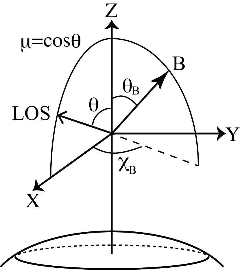
Figure 1: Geometry for the scattering event. The $Z$-axis is normal to the solar surface. The magnetic field vector is characterized by its magnitude $B$, inclination angle $\theta_{B}$, and azimuth $\chi_{B}$. The LOS lies in the $X-Z$ plane. We choose the $Y$-axis as positive reference direction for Stokes $Q$, which is parallel to the nearest solar limb.

By solving the above-mentioned non-local thermodynamic equilibrium (non-LTE) radiative transfer problem, we created a database of synthetic Stokes profiles ($I(\lambda)$, $Q(\lambda)$, and $U(\lambda)$) of the hydrogen Lyman-$\alpha$ line. We consider the presence of a deterministic magnetic field of arbitrary strength $B$, inclination $\theta_{B}$, and azimuth $\chi_{B}$, all of which are assumed to be constant with height (Fig.1). In total, there are 137751 sets of $Q(\lambda)/I(\lambda)$ and $U(\lambda)/I(\lambda)$ profiles for different magnetic field strengths ($0\leq B\leq 250~{}\mathrm{G}$ in $5~{}\mathrm{G}$ increments), inclinations ($0^{\circ}\leq\theta_{B}\leq 180^{\circ}$ in $5^{\circ}$ increments), and azimuths ($0^{\circ}\leq\chi_{B}\leq 360^{\circ}$ in $5^{\circ}$ increments). An example of a synthetic profile is given in Figure 2 (solid lines). For all magnetic parameters, the Stokes $I(\lambda)$ profiles are virtually identical because only the polarization signals have a measurable sensitivity to the magnetic field. Here, we consider two scattering geometries: disk center ($\mu=1.0$) and close-to-the-limb ($\mu=0.3$).

Here, we also simulate the CLASP observations. The wavelength resolution of the CLASP optics is $\sim 0.013$ nm, and the Stokes spectra are recorded with a wavelength sampling of 0.005 nm pixel^-1. For a spatial area of less than 10″, the polarization sensitivity is 0.1% with respect to the intensity at each wavelength pixel in the line core ($121.567\pm 0.02$ nm). First, the synthetic profiles $I(\lambda),Q(\lambda)$, and $U(\lambda)$ in the database are convolved with a 0.013 nm FWHM Gaussian and are then sampled with a wavelength step of 0.005 nm. Assuming that the polarization sensitivity will be achieved at a $3\sigma$ level, random noise with a standard deviation of $\sigma=0.033\%$ with respect to the intensity at each wavelength bin is added to the convolved $I$, $Q$, and $U$ profiles. Finally, we derive the simulated $Q^{obs}(\lambda)/I^{obs}(\lambda)$ and $U^{obs}(\lambda)/I^{obs}(\lambda)$ profiles (squares in Fig.2).

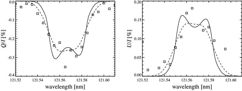
Figure 2: The original synthetic Lyman-$\alpha$ $Q/I$ and $U/I$ profiles (solid lines) for a LOS with $\mu=0.3$, considering the Hanle effect of a 50 G horizontal magnetic field with an azimuth of $120^{\circ}$. The $Q/I$ and $U/I$ convolved with a 0.013 nm FWHM Gaussian are shown with dashed lines. The simulation of the observed profiles (squares), taking into account 0.005-nm pixel samplings and the random noise of $\sigma=0.033\%$.

4 Hanle diagrams

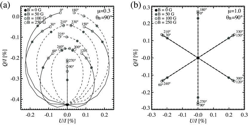
Figure 3: The Hanle diagrams of the hydrogen Lyman-$\alpha$ line at a close-to-the-limb geometry ($\mu=0.3$, (a)) and at the disk center ($\mu=1.0$, (b)) for the case of horizontal magnetic fields ($\theta_{B}=90^{\circ}$). The curves result from the computation of synthetic $Q/I$ and $U/I$ line-center signals for various azimuth $\chi_{B}$ values and field strengths $B$. The lines show the variation of $Q/I$ and $U/I$ as a function of $B$ from $0$ G to $250$ G with constant $\chi_{B}$. The black, dark gray, light gray, and white circles refer to $Q/I$ and $U/I$ for $B=0$, $50$ G, $100$ G, and $250$ G, respectively. The values close to the white circle show $\chi_{B}$ in degrees for each curve. The solid and dashed curves represent cases for $0-150^{\circ}$ and $180-330^{\circ}$, respectively.

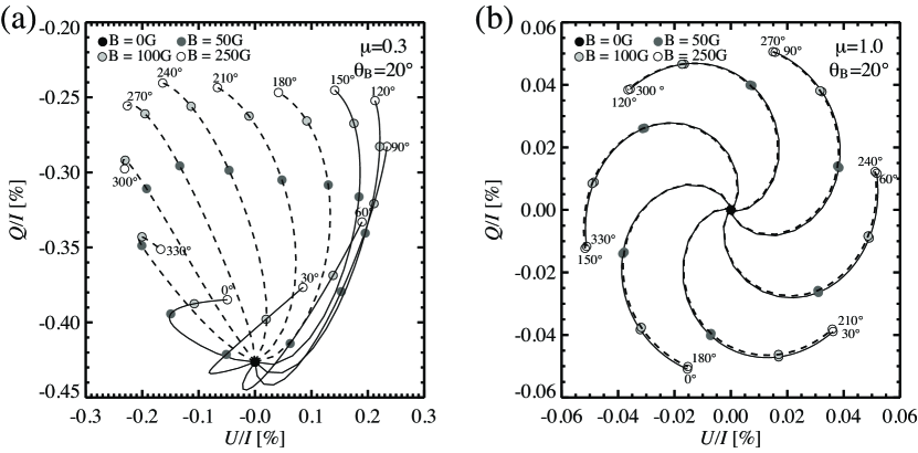
Figure 4: Hanle diagrams for the case of a nearly vertical field ($\theta_{B}=20^{\circ}$). The curves were generated in the same way as those in Figure 3.

The behavior of the $Q/I$ and $U/I$ signals with respect to the magnetic field parameters (strength, inclination, and azimuth of the magnetic field vector) can be suitably illustrated by a Hanle diagram (see also Trujillo Bueno et al., 2012). In Figure 3, we show Hanle diagrams with a horizontal magnetic field (i.e., the inclination is fixed at $\theta_{B}=90^{\circ}$) for different values of the azimuth angle when the field strength varies between 0 G (black circles) and 250 G (white circles). The Figure 3 (a) corresponds to a close-to-limb geometry ($\mu=0.3$), while Figure 3 (b) refers to the forward scattering case of a disk center observation ($\mu=1.0$). The $Q/I$ and $U/I$ signals in this figure refer to the amplitudes of original synthetic profiles $Q(\lambda_{0})/I(\lambda_{0})$ and $U(\lambda_{0})/I(\lambda_{0})$ in the database at the line center, where $\lambda_{0}=121.567$ nm. Figure 4 is similar to Figure 3, but the magnetic field is nearly vertical (i.e., the inclination is fixed at $\theta_{B}=20^{\circ}$).

For the close-to-limb geometry ($\mu=0.3$), the unmagnetized case ($B=0$ G) shown in black circles in Figs. 3 (a) and 4 (a) yields negative Stokes $Q/I$ values, which indicates that the direction of linear polarization caused by the anisotropic radiation field (i.e., the non-magnetic scattering polarization) is perpendicular to the solar limb. As shown by Trujillo Bueno et al. (2011), the anisotropy of the radiation field, $J^{2}_{0}$, illuminating the hydrogen atoms in the Lyman-$\alpha$ line is negative (dominated by horizontal illumination) through the line formation region of the FAL-C model atmosphere. The resulting scattering polarization is perpendicular to the limb. At the disk center ($\mu=1.0$), where the line of sight (LOS) is parallel to the solar normal (i.e., the symmetry axis of the radiation field), we have $Q/I=0$ and $U/I=0$ for the non-magnetized case (black circles in Figs. 3 (b) and 4 (b)).

The crossing points seen in the $\mu=0.3$ Hanle diagrams indicate ambiguity, which occurs when different magnetic field vectors give the same Stokes $Q/I$ and $U/I$ signals. For example, in Figure 3 (a), the crossing point at $Q/I\sim-0.3\%$ and $U/I\sim-0.15\%$ corresponds to cases with $\chi_{B}=330^{\circ}$ and $B=10$ G and with $\chi_{B}=60^{\circ}$ and $B=30$ G. This ambiguity cannot be solved without using additional information to constrain one of magnetic parameters. At the solar disk center ($\mu=1.0$), we have $180^{\circ}$ ambiguity, where two magnetic field vectors whose azimuths differ by $180^{\circ}$ represent the same $Q/I$ and $U/I$ signals (see overlapping solid and dashed lines in Figs. 3 (b) and 4 (b)).

In such Hanle diagrams, the change in linear polarization from $0$ G to $50$ G is larger than that from $50$ G to $250$ G, with the exception of nearly vertical fields in the $\mu=1.0$ forward scattering geometry case (Figure 4 (b)). This trend is prominent for the horizontal field case shown in Figure 3, where $Q/I$ and $U/I$ significantly change from 0 to 50 G but show little change from 50 G to 250 G. This indicates that the Hanle effect in the hydrogen Lyman-$\alpha$ line is sensitive to field strengths $B{<}50$ G. A field strength of $\sim 50$ G corresponds to the critical field strength for the onset of the Hanle effect in the Lyman-$\alpha$ line. Above this field strength, the Lyman-$\alpha$ line approaches the Hanle saturation limit, where the linear polarization is insensitive to the magnetic field strength.

The linear polarization signals produced by the Hanle effect are weaker than 0.1% for a nearly vertical field at the solar disk center ($\mu=1.0$) (Figure 4 (b)) because weak vertical fields do not give rise to a strong symmetry breaking. At the solar disk center, largely inclined and strong fields are more suitable observing targets.

5 Inversion

5.1 General approach for solving the inversion problem

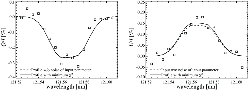
Figure 5: The dashed lines show the convolved synthetic profiles for input with the magnetic parameters of $B=50$ G, $\theta_{B}=90^{\circ}$, and $\chi_{B}=120^{\circ}$. The simulation of the observed profiles (noise with $\sigma=0.033\%$ is added into the input profiles) is shown with squares. The solid lines show the convolved synthetic profiles for one of acceptable solutions with numerically minimal $\chi^{2}$ values (shown with the gray triangle in Figure 6).

To clarify whether we can retrieve information on the magnetic field from the observed Stokes profiles, we perform a process that mimics the Stokes inversion. Here, we assume that the formation of the Lyman-$\alpha$ line is modeled with a semi-empirical FAL-C model atmosphere. For this purpose, we introduce the following function:

$$\chi^{2}(B,\chi_{B},\theta_{B})\equiv\sum_{k=1}^{2}\sum_{l=1}^{n}\frac{[S_{k}^{obs}(\lambda_{l})-S_{k}^{mod}(\lambda_{l},B,\chi_{B},\theta_{B})]^{2}}{\sigma^{2}},$$ (3)

where $S_{1}$ and $S_{2}$ indicate $Q/I$ and $U/I$, respectively. The simulated CLASP observation is $S_{k}^{obs}$ ($k=1,2$), i.e., the synthetic Stokes profile taken from the database, convolved with a 0.013 nm FWHM Gaussian, sampled with a wavelength step of 0.005 nm, with added noise (Section 3). Here, $S_{k}^{mod}$ represents the noiseless model profile corresponding to the synthetic profile convolved with a 0.013 nm FWHM Gaussian and sampled with a wavelength step of 0.005 nm. In the database, the parameter increments in the synthetic profiles are 5 G increments of field strength and 5^∘ increments of azimuth and inclination. In order to have better accuracy in the inversion, $S_{k}^{mod}$ are calculated with $1^{\circ}$ steps for azimuth and inclination and with $1$ G steps for field strength by linearly interpolating model profiles with adjacent magnetic parameters. We take into account the wavelength range of $121.567~{}\mathrm{nm}\pm 0.04~{}\mathrm{nm}$ where the linear polarization signals are defined, resulting in $n=17$ wavelength points. Finally, $\sigma$ is the standard deviation of the random noise we assumed in the CLASP observation simultations. We employ $\sigma=0.033\%$ as the baseline, and in Section 5.4, we will discuss the influence of noise on the inversion results.

We calculate the $\chi^{2}$ function using the given observed profile ($S_{k}^{obs}$) and all of the model profiles ($S_{k}^{mod}$). We find the magnetic parameters with a statistically acceptable $\chi^{2}$, defined by $\Delta\chi^{2}\equiv\chi^{2}-\chi^{2}_{\mathrm{min}}\leq 3.53$, where $\chi^{2}_{\mathrm{min}}$ is the minimum $\chi^{2}$ (Press et al., 2007). Because we have three free parameters ($B$, $\chi_{B}$, and $\theta_{B}$), $\Delta\chi^{2}\equiv\chi^{2}-\chi^{2}_{\mathrm{min}}\leq 3.53$ is given by the chi-square distribution function for three degrees of freedom with a confidence level of 68.3% ($1\sigma$). The parameter region defined by this criteria indicates that there is a 68.3% ($1\sigma$) chance for the true field strength, azimuth, and inclination parameters to fall within this region. We call this procedure “inversion” throughout this paper. Furthermore, we use the term “input” to refer to the magnetic parameters of the simulated observation $S_{k}^{obs}$.

Figure 6: The $\chi^{2}$ map in the field strength, azimuth, and inclination parameter space. The magnetic parameters with $\Delta\chi^{2}\leq 3.53$ (see Section 5.1) are shown in black. The input magnetic parameters of $B=50$ G, $\theta_{B}=90^{\circ}$, and $\chi_{B}=120^{\circ}$ are shown with a gray circle. The gray triangle shows one of the acceptable solutions (magnetic parameter with numerically minimal $\chi^{2}$).

Figure 6 shows the dependence of $\chi^{2}$ on inclination, azimuth, and field strength for the input parameters of $B=50$ G, $\theta_{B}=90^{\circ}$, and $\chi_{B}=120^{\circ}$, which are shown by gray circles. The black region in Figure 6 is defined by $\Delta\chi^{2}\equiv\chi^{2}-\chi^{2}_{\mathrm{min}}\leq 3.53$. The model profiles located in this region fit the simultated observations reasonably well, and all magnetic parameters are statistically accepted as results of inversion with a confidence level of 68% ($1\sigma$). The model profiles corresponding to the input parameters are shown with dashed lines in Figure 5. The magnetic parameters (chosen as an example in the acceptable $\chi^{2}$ region) marked by gray triangle in Figure 6 correspond to the model profiles shown with solid lines in Figure 5. Within the noise level, these profiles are identical.

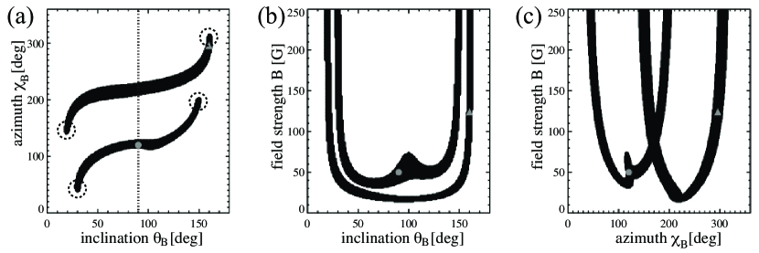
Figure 7: The $\chi^{2}$ maps projected onto the parameter space of (a) inclination and azimuth, (b) inclination and field strength, and (c) azimuth and field strength for the input parameters of $B=50$ G, $\theta_{B}=90^{\circ}$, and $\chi_{B}=120^{\circ}$. The regions with $\Delta\chi^{2}\leq 3.53$ are shown in black. The input magnetic parameters are shown with gray circles. The gray triangle represents one of acceptable solutions shown in Figure 6. The four dashed circles in panel (a) indicate the four ambiguous solutions in saturation regime.

5.2 Properties of the $\chi^{2}$ map

5.2.1 Saturation regime

Figure 7 represents the $\chi^{2}$ maps projected onto two parameter spaces. There are four 1$\sigma$ confidence level regions ($\Delta\chi^{2}\leq 3.53$) extended along the field strength above 50 G at $\theta_{B}=20^{\circ}$, $30^{\circ}$, $150^{\circ}$, $155^{\circ}$ in Figure 7 (b) and at $\chi_{B}=40^{\circ}$, $145^{\circ}$, $195^{\circ}$, $310^{\circ}$ in Figure 7 (c). The four dashed circles in Figure 7 (a) show the regions on the $\theta_{B}$-$\chi_{B}$ plane where $(\theta_{B},\chi_{B})=\{(20^{\circ},145^{\circ}),(30^{\circ},40^{\circ}),(150^{\circ},195^{\circ}),(155^{\circ},310^{\circ})\}$, indicating four possible solutions of inclination and azimuth above 50 G. The elongated line, which occurs in only field strength direction, indicates a large uncertainty in the field strength where we cannot constrain the field strength. In other words, we do not have sensitivity to measure the magnetic field strength beyond $\sim 50$ G. Multiple simply-connected spaces ($1\sigma$ confidence level regions) indicate the ambiguity of solutions in which completely different magnetic parameters provide the same $Q/I$ and $U/I$ profiles.

The elongated regions correspond to the saturation regime, in which the linear polarization weakly depends on the field strength. This is consistent with the Hanle diagrams (Section 4), where the change of linear polarization above 50 G is small compared with that below 50 G. In this saturation regime, the linear polarization signal is only dependent on the inclination and azimuth. Thus, we can determine the azimuth and inclination. However, ambiguity allows four combinations of inclination and azimuth to exist as shown in Figure 7. The ambiguity corresponds to the Van Vleck ambiguity in the saturation regime, which is inherent to the Hanle effect. These four ambiguous solutions provide magnetic parameters with less inclined ($\theta_{B}\sim 20-30^{\circ}$ or $\theta_{B}\sim 150-160^{\circ}$) and relatively strong ($B>50$ G) magnetic field vectors.

5.2.2 Non-saturation regime

Below 50 G, the linear polarization of $Q/I$ and $U/I$ depends on the field strength as well as on the inclination and azimuth (Section 4); this is the non-saturation regime. As shown in Figure 7 (a), in the non-saturation regime, there are two isolated $1\sigma$ confidence level regions with saturation regimes at both ends (dashed circles, four in total). These two isolated regions are elongated over the wide inclination and azimuth range on the $\theta_{B}$-$\chi_{B}$ plane. Different magnetic parameters give rise to the same linear polarization signals in these two regions. This can be confirmed by the Hanle diagram in Figure 3 (a). If we assume that the magnetic field is horizontal ($\theta_{B}=90^{\circ}$), as shown in the dashed line in Figure 7 (a), two solutions are possible: one for $\chi_{B}=120^{\circ}$ and $B=50$ G (shown in gray circle) and the other for $\chi_{B}=225^{\circ}$ and $B=15$ G. Indeed, the Hanle diagram with $\chi_{B}=120^{\circ}$ and $B=50$ G intersects with that with $\chi_{B}=225^{\circ}$ and $B=15$ G, suggesting the presence of ambiguity.

Below $\sim 50$ G, Figure 7 (b) shows that one $1\sigma$ confidence level region, which extends from $\theta_{B}\sim 20^{\circ}$ to $\theta_{B}\sim 150^{\circ}$, has an apex at $B\sim 15$ G and $\theta_{B}\sim 90^{\circ}$. Figure 7 (b) further shows that another $1\sigma$ confidence level region, which extends in the $\theta_{B}=30^{\circ}$ to $140^{\circ}$ range, possesses two vertices at $\theta_{B}\sim 60^{\circ}$ and $\theta_{B}\sim 120^{\circ}$. The elongated shape over the inclination and field strength shows a strong correlation between these two magnetic parameters; both a weak and inclined field and a stronger and less inclined field provide equally good fitting to the observed spectra. On the $\chi_{B}$-$B$ plane, the two $1\sigma$ confidence level regions have a V-shape with apexes at $\chi_{B}\sim 120^{\circ}$ and $B\sim 40$ G and at $\chi_{B}\sim 220^{\circ}$ and $B\sim 15$ G. This also suggests that there is a correlation between the azimuth and field strength and that the wide field strength range is consistent with the data. We notice that the azimuth converges to $120^{\circ}$ or $220^{\circ}$ when the field strength becomes weaker. In general, there is strong correlation among these three magnetic parameters, and it is difficult to uniquely determine a set of these magnetic parameters.

5.2.3 Connection between saturation and non-saturation regimes

We find four-fold ambiguity in the saturation regime ($B>50$ G) and two-fold ambiguity in the non-saturation regime ($B<50$ G). As we clearly show in Figure 6, a pair of saturated regimes converges into one of the non-saturated regimes (there are two sets of connections). This connectivity indicates that the Stokes $Q/I$ and $U/I$ profiles for a strong and less inclined magnetic field is similar to those of a weaker and more inclined field. This transition suggests that the degree of the Hanle effect remains the same among strong, less inclined fields and weaker, more inclined fields. In summary, multiple solutions are possible over a broad field strength range. In the saturation regime ($B>50$ G), we can only determine the azimuth and inclination, although we have multiple solutions in these parameters. As we enter the non-saturation regime, we have strong correlations among three magnetic parameters in addition to the above ambiguity. These situations make it difficult to uniquely determine the magnetic field vector.

5.3 Additional information for constraining magnetic parameters

If there are multiple solutions, one way to uniquely determine the magnetic field vector is to constrain one of parameters using additional observations. With the exception of the saturation regime, the 1$\sigma$ confidence level regions are extended over the three-dimensional parameter space as shown in the 2D $\chi^{2}$ maps in Figure 7. The shape helps us to constrain the magnetic parameters with an additional piece of information. For example, once the azimuth is constrained by other observations, the inclination and field strength will be uniquely determined as inferred from Figure 7 (a) and (c). An accuracy of $\pm 5^{\circ}$ in the azimuthal direction will be good enough for most cases. However, when $\chi_{B}=215^{\circ}$ and $\chi_{B}=120^{\circ}$, the correlation curve on the plane of inclination and azimuth allows a relatively large uncertainty in the inclination (see Fig.7 (a)).

The Lyman-$\alpha$ images of the upper chromosphere obtained with the Very high Angular resolution ULtraviolet Telescope (VAULT) sounding rocket (Vourlidas et al., 2010) show the presence of long thin threads of $\sim 10\arcsec$ in the quiet Sun. The Mg II k and Ca II images obtained with the Sunrise FilterImager (SuFI; Gandorfer et al., 2011) revealed fibril structures spreading from the plage regions in the chromosphere (Riethmüller et al., 2013). As shown by Leenaarts et al. (2012, 2013), the magnetic field connecting magnetic concentrations with opposite polarities represents the intensity filamentary structure in their 3D atmospheric model. This indicates that the intensity filamentary structures can be used as proxies of the azimuth of the magnetic fields. Therefore, high-spatial resolution observations around the line forming layer of the Lyman-$\alpha$ line would help us to know the azimuthal direction. The CLASP Lyman-$\alpha$ slit-jaw images, the Interface Region Imaging Spectrograph (IRIS), the Atmospheric Imaging Assembly (AIA) onboard the Solar Dynamics Observatory (SDO), and ground-based observations can be used for this purpose.

5.4 Inversion with different noise levels

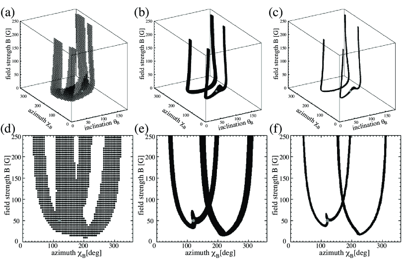
Figure 8: The $\chi^{2}$ maps in the field strength, azimuth, and inclination parameter space with the input parameters of $B=50$ G, $\theta_{B}=90^{\circ}$, and $\chi_{B}=120^{\circ}$ at $\mu=0.3$ are shown for three different noise levels: (a) $1\sigma=0.1\%$, (b) $1\sigma=0.03\%$, and (c) $1\sigma=0.01\%$. (d), (e), and (f) are the $\chi^{2}$ maps from (a), (b), and (c), respectively, projected onto the azimuth and field strength parameter space. In (a) and (d), the regions with $\Delta\chi^{2}\leq 3.53$ are plotted with $5^{\circ}$ increments in $\chi_{B}$ and $\theta_{B}$ and with 5 G increments in $B$. The input magnetic parameters are shown with gray circles in all panels.

Here, we investigate the influence of the noise level on the inversion results. Figure 8 represents the dependence of the $\chi^{2}$ values on inclination, azimuth, and field strength for noise levels of $1\sigma=0.1\%$, $1\sigma=0.03\%$, and $1\sigma=0.01\%$. The input parameters for all cases are $B=50$ G, $\theta_{B}=90^{\circ}$, and $\chi_{B}=120^{\circ}$. Note that Figure 8 (b) is the same as Figure 6. The $\chi^{2}$ distributions are similar for all noise levels. Above 50 G, four isolated $1\sigma$ confidence regions with $\Delta\chi^{2}\leq 3.53$ are extended only in the direction of the field strength, representing the saturation regime. Around 50 G, these regions are connected to the two isolated regions with largely inclined, weak fields. Even though we increase the signal-to-noise ratio, the ambiguity remains intact, and we find similar correlation between the magnetic parameters. Thus, we require additional observables to constrain the solution even in low noise situations. The difference caused by different noise levels is equivalent to the thickness of the $1\sigma$ confidence level region. These regions are thinner for lower noise levels, indicating lower uncertainty in the determination of the magnetic parameters. For example, in the saturation regime, the thicknesses correspond to $40^{\circ}$ for $1\sigma=0.1\%$, $\sim$10^∘ for $1\sigma=0.033\%$, and $\sim$5^∘ for $1\sigma=0.01\%$ (see Figure 8 (d), (e) and (f)).

5.5 Inversion for different observing regions and input parameters

To see whether the properties of the $\chi^{2}$ maps (i.e., result of inversion) identified in Section 5.2 depend on the choice of the input parameters, we perform inversions for different sets of input parameters and for different observing locations on the solar disk. We study input parameters with weak field ($B=10$ G), marginal field ($B=50$ G), and strong field ($B=250$ G) with both horizontal ($\theta_{B}=90^{\circ}$) and almost vertical ($\theta_{B}=20^{\circ}$) configurations. Note that all azimuths are fixed at $\chi_{B}=120^{\circ}$. With this set of input parameters, we consider both the close-to-limb case ($\mu=0.3$) and the disk center case ($\mu=1.0$) and execute 12 total inversions.

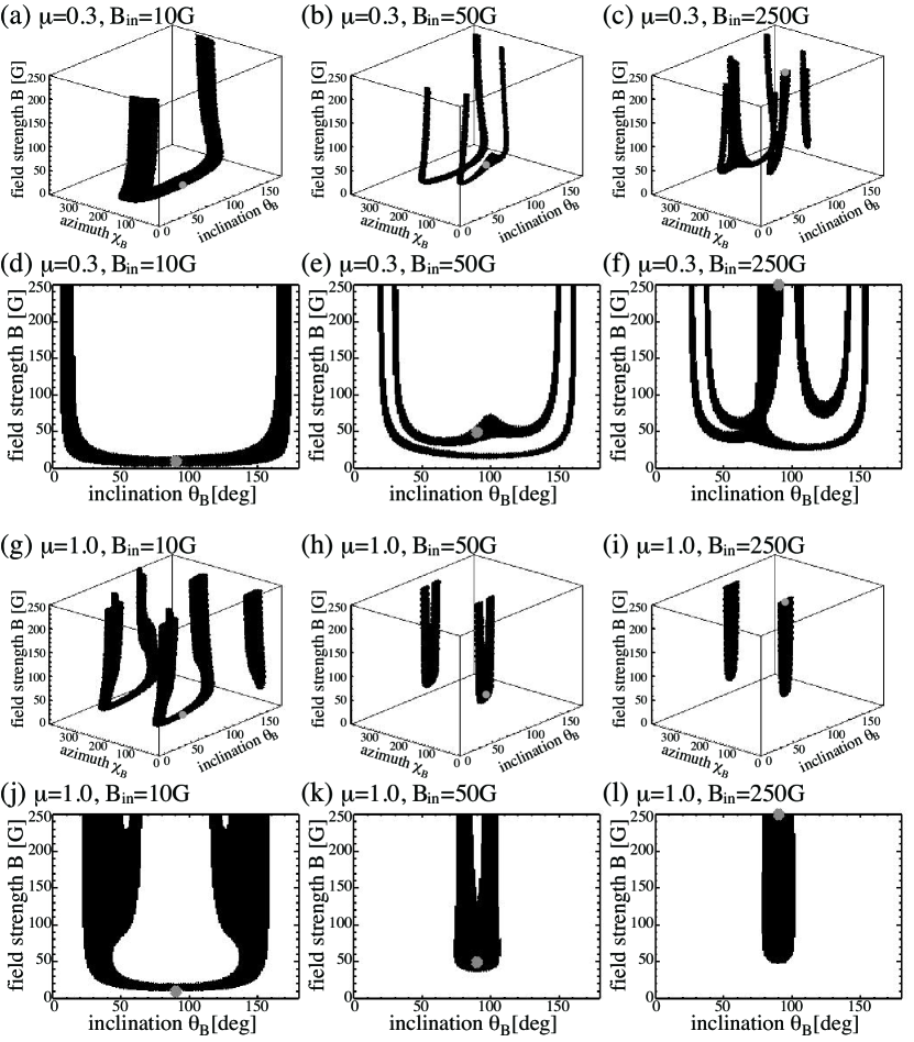
Figure 9: Plots (a), (b), and (c), and plots (g), (h), and (i) represent the $\chi^{2}$ maps in the field strength, azimuth, and inclination parameter space for a horizontal magnetic field ($\theta_{B}=90^{\circ}$) input with the close-to-limb ($\mu=0.3$) and the disk center ($\mu=1.0$) geometries, respectively. Plots (d), (e), and (f) and plots (j), (k), and (l) represent the $\chi^{2}$ maps projected onto the inclination and field strength parameter space. The left, middle, and right columns show $\chi^{2}$ maps with a noise level of $\sigma=0.033\%$ for the inputs of weak field ($B=10$ G), marginal field ($B=50$ G), and strong field ($B=250$ G), respectively, The black regions represent the magnetic parameters with $\Delta\chi^{2}\leq 3.53$. The input magnetic parameters are shown with gray circles.

Figure 9 shows $\chi^{2}$ maps for the case of a horizontal magnetic field. With the exception of the disk center case ($\mu=1.0$) with $B=50$ G (Figure 9 (h) and (k)) and $B=250$ G (Figure 9 (i) and (l)), the $\chi^{2}$ distributions are similar to those in Section 5.2, and any field strength, from weak to strong, is consistent with the data. For the disk center, with horizontal magnetic fields of 50 and 250 G, the $1\sigma$ confidence level region appears only in the saturation regime. Thus, in this case, there is no possibility to have a wrong solution with weak magnetic fields. This is distinct advantage; however, is impossible to determine the field strength in this case. The number of ambiguous regions is different depending on the input parameters.

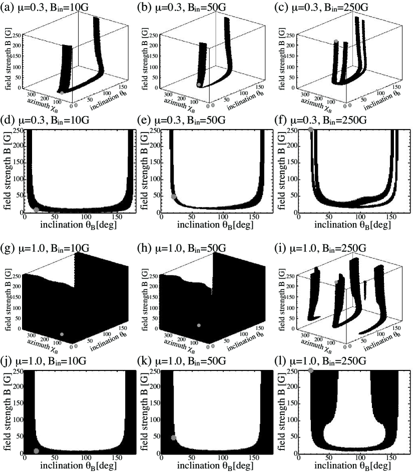
Figure 10: The plots shown here are the same as those in Figure 9 with an almost vertical magnetic field ($\theta_{B}=20^{\circ}$) input value.

Figure 10 shows $\chi^{2}$ maps for the case of vertical magnetic fields ($\theta_{B}=20^{\circ}$). Again, we find the same properties of $\chi^{2}$ distributions, indicating that any field strength can be possible as a solution. For the disk center case with $B=10$ G and $B=50$ G (Figure 10 (g) and (h)), the $1\sigma$ confidence regions with $\Delta\chi^{2}\leq 3.53$ spread out on the plane with vertical fields ($\theta_{B}=0^{\circ}$ or $\theta_{B}=180^{\circ}$) and on the plane with zero magnetic fields (see Figure 10 (j) and (k)), indicating that the inversion does not work. This result is reasonable because the the magnitude of linear polarization is quite small and below the noise level when the magnetic fields are almost vertical, as shown in Figure 4 (b). If we employ a smaller noise level, properties of the $\chi^{2}$ distribution similar to those in Section 5.2 will appear. For CLASP observations, an observing target with a largely inclined and/or strong magnetic field strength is appropriate for the disk center observation.

6 Discussions

6.1 Required additional information

We have performed Stokes inversion simulations to clarify the information which can be inferred via the Hanle effect in the hydrogen Lyman-$\alpha$ line, assuming that the chromosphere and transition region of the quiet Sun can be represented by the FAL-C semi-empirical model. We conclude that UV spectro-polarimetry with the CLASP experiment is a suitable diagnostic tool of the magnetic field in the upper atmosphere, if combined with complementary information from other relevant observations. Though we have the ambiguity and uncertainty that is inherent to the Hanle effect when only the scattering polarization in one spectral line is available, this should not be taken as a drawback. As we have shown, we need additional observations to uniquely determine the field strength, azimuth, and inclination. Clearly, we cannot measure the very small contribution of the Zeeman effect to the Stokes $V$ of the Lyman-$\alpha$ line, but there are several options for resolving this issue. Ideally, we would like to perform simultaneous spectro-polarimeteric observations also in other spectral lines of the upper chromosphere, which have different critical field strengths for the onset of the Hanle effect (Trujillo Bueno et al., 2012; Belluzzi & Trujillo Bueno, 2012). However, in this paper, we propose a simpler, but useful, third method for determining the azimuthal magnetic field direction using the fibrils seen in the high-resolution intensity images from IRIS, AIA, and ground-based observations.

6.2 Observing target

The Lyman-$\alpha$ line starts to approach the Hanle saturation regime above $\sim$50 G, where the linear polarization changes only with the inclination and azimuth of the magnetic field, not with its strength. Furthermore, nearly vertical fields do not produce any significant Hanle effect (i.e., the magnetic modification of the linear polarization), and at the solar disk center the linear polarization created by the Hanle effect of slightly inclined fields is too small to be detected. Thus, inclined, relatively weak ($B<50$ G) magnetic fields should be observed. Based on the properties of the Hanle effect studied in this paper, we can now discuss the possible observing region and observing target for the CLASP experiment.

Our primary goal with the CLASP experiment is to detect for the first time the linear polarization caused by the atomic level polarization produced by the absorption and scattering of anisotropic radiation in the upper solar atmosphere. To this end, it is desirable to choose a quiet region close to the limb (e.g., around $\mu{\approx}0.3$) because such locations are the most suitable ones for detecting the line-core polarization in the hydrogen Lyman-$\alpha$ line (Trujillo Bueno et al., 2011; Belluzzi et al., 2012; Štěpán et al., 2014). Our second goal is to detect the Hanle effect, in order to constrain the magnetic field vector of the chromosphere-corona transition region.

One of the popular spectral lines for magnetic field measurements in the upper atmosphere is the He i 1083 nm triplet (e.g., Asensio Ramos et al., 2008). By exploiting the spectro-polarimetric data obtained with this multiplet, the magnetic properties of prominences, filaments, spicules and active regions have been investigated by several authors (e.g., Trujillo Bueno et al., 2002; Lagg et al., 2004; Merenda et al., 2006; Centeno et al., 2010; Xu et al., 2010). However, it is not easy to measure the intensity and polarization of the He i 1083 nm triplet in quiet regions of the solar disk (e.g., Asensio Ramos et al., 2008), and there are few studies on the quiet-Sun magnetic fields of the upper solar atmosphere. Thus, our primary targets are the network and internetwork regions of the quiet Sun. The network fields are expected to form magnetic canopy structures in the upper chromosphere and transition region, and they are expected to be largely inclined and relatively weak. Wiegelmann et al. (2010) investigated the fine structure of the magnetic fields in the quiet Sun using photospheric magnetic field measurements from the SUNRISE imaging magnetograph experiment (IMaX). Wiegelmann et al. (2010) found that most magnetic loops rooted in the quiet Sun photosphere would reach into the chromosphere or higher. In addition to the canopy field, such magnetic loops in regions of the quiet Sun would also be interesting observing targets.

6.3 Atmospheric model

Finally, we discuss another issue that we should address further in future investigations: the influence of the atmospheric model on the inference of the magnetic field via the interpretation of the scattering polarization and the Hanle effect in Lyman-$\alpha$. Belluzzi et al. (2012) calculated the scattering polarization profiles of the hydrogen Lyman-$\alpha$ line taking into account partial frequency redistribution (PRD) and $J-$state interference effects, and using the plane-parallel atmospheric models C, F, and P of Fontenla et al. (1993), which can be considered as illustrative of quiet, network, and plage regions. They showed that the shape and amplitude of the Lyman-$\alpha$ linear polarization profiles are sensitive to the thermal structure of the model atmosphere in the line wings, and to a lesser extent also in the line core (where the Hanle effect operates). Thus, in order to determine the importance of the choice of the atmospheric model, we must clarify how much uncertainty arises in the inference of the magnetic field vector when the chosen atmospheric model is different.

It is important to emphasize that the upper solar chromosphere and transition region are highly inhomogeneous and dynamic plasmas. Such inhomogeneity and dynamics causes larger $Q/I$ amplitudes and non-zero $U/I$ signals, along which their spatial and temporal variations (Štěpán et al., 2012, 2014). Thus, we must consider also other strategies for interpreting the CLASP observations, such as detailed forward modeling of the observed scattering polarization signals using increasingly realistic 3D models of the solar chromosphere, taking into account the limited spatial and temporal resolution of the CLASP observations.

In order to monitor the local non-uniformity of the Lyman-$\alpha$ radiation field, the intensity images from the CLASP slit-jaw and IRIS observations will be useful. Furthermore, the intensity and the linear polarization profiles in the line wings, which are insensitive to the magnetic field but very sensitive to the temperature structure, may also help us to constrain the temperature structure of the solar atmosphere. All these steps will facilitate the interpretation of the line-core polarization signals of Lyman-$\alpha$ that CLASP aims at observing. In this way, we expect that the CLASP experiment will lead to the first significant advancement in the investigation of the magnetism of the upper solar chromosphere and the transition region via the Hanle effect in the UV spectral region.

References

- Anusha et al. (2011) Anusha, L. S., Nagendra, K. N., Bianda, M., et al. 2011, ApJ, 737, 95
- Asensio Ramos et al. (2008) Asensio Ramos, A., Trujillo Bueno, J., & Landi Degl’Innocenti, E. 2008, ApJ, 683, 542
- Belluzzi & Trujillo Bueno (2012) Belluzzi, L., & Trujillo Bueno, J. 2012, ApJ, 750, L11
- Belluzzi et al. (2012) Belluzzi, L., Trujillo Bueno, J., & Štěpán, J. 2012, ApJ, 755, L2
- Carlsson & Stein (1997) Carlsson, M., & Stein, R. F. 1997, ApJ, 481, 500
- Casini & Landi Degl’Innocenti (2008) Casini, R., & Landi Degl’Innocenti, E. 2008, in Plasma Polarization Spectroscopy, ed. T. Fujimoto, & A. Iwamae (Atomic, Optical, and Plasma Physics), 44
- Centeno et al. (2010) Centeno, R., Trujillo Bueno, J., & Asensio Ramos, A. 2010, ApJ, 708, 1579
- De Pontieu et al. (2007) De Pontieu, B., McIntosh, S. W., Carlsson, M., et al. 2007, Science, 318, 1574
- Fontenla et al. (1993) Fontenla, J. M., Avrett, E. H., & Loeser, R. 1993, ApJ, 406, 319
- Gandorfer et al. (2011) Gandorfer, A., Grauf, B., Barthol, P., et al. 2011, Sol. Phys., 268, 35
- Ishikawa et al. (2011) Ishikawa, R., Bando, T., Fujimura, D., et al. 2011, Solar Polarization 6, 437, 287
- Kano et al. (2012) Kano, R., Bando, T., Narukage, N., et al. 2012, Proc. SPIE, 8443,
- Katsukawa et al. (2007) Katsukawa, Y., Berger, T. E., Ichimoto, K., et al. 2007, Science, 318, 1594
- Kobayashi et al. (2012) Kobayashi, K., Kano, R., Trujillo Bueno, J., et al. 2012, in Hinode 5, ASP Conf. Series Vol. 456, ed. Leon Golub, Ineke De Moortel, & Toshifumi Shimizu. San Francisco: Astronomical Society of the Pacific, 2012., p.233
- Lagg et al. (2004) Lagg, A., Woch, J., Krupp, N., & Solanki, S. K. 2004, A&A, 414, 1109
- Landi Degl’Innocenti & Landolfi (2004) Landi Degl’Innocenti, E., & Landolfi, M. 2004, Astrophysics and Space Science Library, 307,
- Landi Degl’Innocenti (1982) Landi Degl’Innocenti, E. 1982, Sol. Phys., 79, 291
- Landi Degl’Innocenti & Bommier (1993) Landi Degl’Innocenti, E., & Bommier, V. 1993, ApJ, 411, L49
- Leenaarts et al. (2012) Leenaarts, J., Carlsson, M., & Rouppe van der Voort, L. 2012, ApJ, 749, 136
- Leenaarts et al. (2013) Leenaarts, J., Pereira, T. M. D., Carlsson, M., Uitenbroek, H., & De Pontieu, B. 2013, ApJ, 772, 90
- López Ariste & Casini (2003) López Ariste, A., & Casini, R. 2003, ApJ, 582, L51
- Merenda et al. (2006) Merenda, L., Trujillo Bueno, J., Landi Degl’Innocenti, E., & Collados, M. 2006, ApJ, 642, 554
- Narukage et al. (2011) Narukage, N., Tsuneta, S., Bando, T., et al. 2011, Proc. SPIE, 8148,
- Okamoto & De Pontieu (2011) Okamoto, T. J., & De Pontieu, B. 2011, ApJ, 736, L24
- Okamoto et al. (2007) Okamoto, T. J., Tsuneta, S., Berger, T. E., et al. 2007, Science, 318, 1577
- Press et al. (2007) Press, W. H., Teukolsky, S. A., Vetterling, W. T., & Flannery, B. P. 2007, Numerical recipes: the art of scientific computing, Cambridge University Press, pp 812–815
- Riethmüller et al. (2013) Riethmüller, T. L., Solanki, S. K., Hirzberger, J., et al. 2013, ApJ, 776, L13
- Shibata et al. (2007) Shibata, K., Nakamura, T., Matsumoto, T., Otsuji, K., Okamoto, T. J., Nishizuka, N., Kawate, T., Watanabe, H., Nagata, S., UeNo, S., Kitai, R., Nozawa, S., Tsuneta, S., Suematsu, Y., Ichimoto, K., Shimizu, T., Katsukawa, Y., Tarbell, T. D., Berger, T. E., Lites, B. W., Shine, R. A., & Title, A. M. 2007, Science, 318, 1591
- Štěpán & Trujillo Bueno (2011) Štěpán, J., & Trujillo Bueno, J. 2011, ApJ, 732, 80
- Štěpán et al. (2012) Štěpán, J., Trujillo Bueno, J., Carlsson, M., & Leenaarts, J. 2012, ApJ, 758, L43
- Štěpán et al. (2014) Štěpán, J., Trujillo Bueno, J., Leenaarts, J., & Carlsson, M. 2014, submitted
- Trujillo Bueno et al. (2002) Trujillo Bueno, J., Landi Degl’Innocenti, E., Collados, M., Merenda, L., & Manso Sainz, R. 2002, Nature, 415, 403
- Trujillo Bueno et al. (2011) Trujillo Bueno, J., Štěpán, J., & Casini, R. 2011, ApJ, 738, L11
- Trujillo Bueno et al. (2012) Trujillo Bueno, J., Štěpán, J., & Belluzzi, L. 2012, ApJ, 746, L9
- Vecchio et al. (2009) Vecchio, A., Cauzzi, G., & Reardon, K. P. 2009, A&A, 494, 269
- Vourlidas et al. (2010) Vourlidas, A., Sanchez Andrade-Nuño, B., Landi, E., et al. 2010, Sol. Phys., 261, 53
- Wiegelmann et al. (2010) Wiegelmann, T., Solanki, S. K., Borrero, J. M., et al. 2010, ApJ, 723, L185
- Xu et al. (2010) Xu, Z., Lagg, A., & Solanki, S. K. 2010, A&A, 520, A77