Threesomes, Degenerates, and Love Triangles

Abstract

The 3SUM problem is to decide, given a set of $n$ real numbers, whether any three sum to zero. It is widely conjectured that a trivial $O(n^{2})$-time algorithm is optimal and over the years the consequences of this conjecture have been revealed. This 3SUM conjecture implies $\Omega(n^{2})$ lower bounds on numerous problems in computational geometry and a variant of the conjecture implies strong lower bounds on triangle enumeration, dynamic graph algorithms, and string matching data structures.

In this paper we refute the 3SUM conjecture. We prove that the decision tree complexity of 3SUM is $O(n^{3/2}\sqrt{\log n})$ and give two subquadratic 3SUM algorithms, a deterministic one running in $O(n^{2}/(\log n/\log\log n)^{2/3})$ time and a randomized one running in $O(n^{2}(\log\log n)^{2}/\log n)$ time with high probability. Our results lead directly to improved bounds for $k$-variate linear degeneracy testing for all odd $k\geq 3$. The problem is to decide, given a linear function $f(x_{1},\ldots,x_{k})=\alpha_{0}+\sum_{1\leq i\leq k}\alpha_{i}x_{i}$ and a set $A\subset\mathbb{R}$, whether $0\in f(A^{k})$. We show the decision tree complexity of this problem is $O(n^{k/2}\sqrt{\log n})$.

Finally, we give a subcubic algorithm for a generalization of the $(\min,+)$-product over real-valued matrices and apply it to the problem of finding zero-weight triangles in weighted graphs. We give a depth-$O(n^{5/2}\sqrt{\log n})$ decision tree for this problem, as well as an algorithm running in time $O(n^{3}(\log\log n)^{2}/\log n)$.

1 Introduction

The time hierarchy theorem [26] implies that there exist problems in $\mathbf{P}$ with complexity $\Omega(n^{k})$ for every fixed $k$. However, it is consistent with current knowledge that all problems of practical interest can be solved in $\tilde{O}(n)$ time in a reasonable model of computation. Efforts to build a useful complexity theory inside $\mathbf{P}$ have been based on the conjectured hardness of certain archetypal problems, such as 3SUM, $(\min,+)$-matrix product, and CNF-SAT. See, for example, the conditional lower bounds in [25, 32, 33, 27, 2, 3, 34, 16, 37].

In this paper we study the complexity of 3SUM and related problems such as linear degeneracy testing (LDT) and finding zero-weight triangles. Let us define the problems formally.

3SUM:

Given a set $A\subset\mathbb{R}$, determine if there exists $a,b,c\in A$ such that $a+b+c=0$.

Integer3SUM:

Given a set $A\subseteq\{-U,\ldots,U\}\subset\mathbb{Z}$, determine if there exists $a,b,c\in A$ such that $a+b+c=0$.

$k$-LDT and $k$-SUM:

Fix a $k$-variate linear function $\phi(x_{1},\ldots,x_{k})=\alpha_{0}+\sum_{i=1}^{k}\alpha_{i}x_{i}$, where $\alpha_{0},\ldots,\alpha_{k}\in\mathbb{R}$. Given a set $A\subset\mathbb{R}$, determine if $\phi(\mathbf{x})=0$ for any $\mathbf{x}\in A^{k}$. When $\phi$ is $\sum_{i=1}^{k}x_{i}$ the problem is called $k$-SUM.

ZeroTriangle:

Given a weighted undirected graph $G=(V,E,w)$, where $w:E\rightarrow\mathbb{R}$, determine if there exists a triangle $(a,b,c)\in V^{3}$ for which $w(a,b)+w(b,c)+w(c,a)=0$. (From the definition of love : a score of zero, one could also call this the LoveTriangle problem.)

These problems are often defined with further constraints that do not change the problem in any substantive way [25]. For example, the input to 3SUM can be three sets $A,B,C\subset\mathbb{R}$ and the problem is to determine if there exists $a\in A,b\in B,c\in C$ such that $a+b+c=0$. Even if there is only one set, there is sometimes an additional constraint that $a,b,$ and $c$ be distinct elements.

As a problem in its own right, 3SUM has no compelling practical applications. However, lower bounds on 3SUM imply lower bounds on dozens of other problems that are of practical interest. Before reviewing existing 3SUM algorithms we give a brief survey of conditional lower bounds that depend on the hardness of 3SUM.

1.1 Implications of the 3SUM Conjectures

It is often conjectured that 3SUM requires $\Omega(n^{2})$ time and that Integer3SUM requires $\Omega(n^{2-o(1)})$ time [32, 3]. These conjectures have been shown to imply strong lower bounds on numerous problems in computational geometry [25, 4, 9, 35] dynamic graph algorithms [32, 3], and pattern matching [1, 6, 14, 17]. For example, the 3SUM conjecture implies that the following problems require at least $\Omega(n^{2})$ time.

1. Given an $n$-point set in $\mathbb{R}^{2}$, determine whether it contains three collinear points [25].

2. Given two $n$-edge convex polygons, determine whether one can be placed inside the other via rotation and translation [9].

3. Given $n$ triangles in $\mathbb{R}^{2}$, determine whether their union contains a hole, or determine the area of their union [25].

Through a series of reductions, Pǎtraşcu [32] proved that the Integer3SUM conjecture implies lower bounds on triangle enumeration and various problems in dynamic data structures, even when all updates and queries are presented in advance. Some lower bounds implied by the Integer3SUM conjecture include the following.

1. Given an undirected $m$-edge graph, enumerating up to $m$ triangles (3-cycles) requires at least $\Omega(m^{4/3-o(1)})$ time [32].

2. Given a sequence of $m$ updates to a directed graph (edge insertions and edge deletions) and two specified vertices $s,t$, determining whether $t$ is reachable from $s$ after each update requires at least $\Omega(m^{4/3-o(1)})$ time [3].

3. Given an edge-weighted undirected graph, deciding whether there exists a zero-weight triangle requires at least $\Omega(n^{3-o(1)})$ time [38].

In recent years conditional lower bounds have been obtained from two other plausible conjectures: that computing the $(\min,+)$-product of two $n\times n$ matrices takes $\Omega(n^{3-o(1)})$ time and that CNF-SAT takes $\Omega(2^{(1-o(1))n})$ time. The latter is sometimes called the Strong Exponential Time Hypothesis (Strong ETH). We now know that if the Strong ETH holds, no $n^{o(k)}$ algorithm exists for $k$-SUM [33] and no $m^{2-\Omega(1)}$ algorithm exists for $(3/2-\epsilon)$-approximating the diameter of an $m$-edge unweighted graph [34, 16]. Williams and Williams [37] proved that numerous problems are equivalent to $(\min,+)$-matrix multiplication, inasmuch as a truly subcubic ($O(n^{3-\Omega(1)})$) algorithm for one would imply truly subcubic algorithms for all the others.

1.2 Algorithms, Lower Bounds, and Reductions

The evidence in favor of the 3SUM and Integer3SUM conjectures is rather thin. Erickson [22] and Ailon and Chazelle [5] proved that any $k$-linear decision tree for solving $k$-LDT must have depth $\Omega(n^{k/2})$ when $k$ is even and $\Omega(n^{(k+1)/2})$ when $k$ is odd. In particular, any 3-linear decision tree for 3SUM has depth $\Omega(n^{2})$. (An $s$-linear decision tree is one where each internal node asks for the sign of a linear expression in $s$ elements.) The Integer3SUM problem is obviously not harder than 3SUM, but no other relationship between these two problems is known. Indeed, the assumption that elements are integers opens the door to a variety of algorithmic techniques that cannot be modeled as decision trees. Using the fast Fourier transform it is possible to solve Integer3SUM in $O(n+U\log U)$ time, which is subquadratic even for a rather large universe size $U$. Baran, Demaine, and Pǎtraşcu [8] showed that Integer3SUM can be solved in $O(n^{2}/(\log n/\log\log n)^{2})$ time (with high probability) on the word RAM, where $U=2^{w}$ and $w>\log n$ is the machine word size. The algorithm uses a mixture of randomized universe reduction (via hashing), word packing, and table lookups.

It is straightforward to reduce $k$-LDT to a 2SUM problem or unbalanced 3SUM problem, depending on whether $k$ is even or odd. When $k$ is odd one forms certain sets $A,B,C$ where $|A|=|B|=n^{(k-1)/2}$ and $|C|=n$, then sorts them in $O(n^{(k-1)/2}\log n)$ time. The standard three-set 3SUM algorithm on $A,B,C$ takes $O(|C|(|A|+|B|))=O(n^{(k+1)/2})$ time. When $k\geq 4$ is even there is no set $C$. Using Lambert’s algorithm [28], $A$ and $B$ can be sorted is $O(n^{k/2}\log n)$ time while performing only $O(n^{k/2})$ comparisons. These algorithms can be modeled as $k$-linear decision trees, and are therefore optimal in this model by the lower bounds of [22, 5]. However, it was known that all $k$-LDT problems can be solved by $n$-linear decision trees with depth $O(n^{5}\log n)$ [29], or with depth $O(n^{4}\log(nK))$ if the coefficients of the linear function are integers with absolute value at most $K$ [30]. Unfortunately these decision trees are not efficiently constructible. The time required to determine which comparisons to make is exponential in $n$.

The ZeroTriangle problem was highlighted in a recent article by Williams and Williams [38]. They did not give any subcubic algorithm, but did show that a subcubic ZeroTriangle algorithm would have implications for Integer3SUM via an intermediate problem called Convolution3SUM.

Convolution3SUM:

Given a vector $A\in\mathbb{R}^{n}$, determine if there exist $i,j$ for which $A(i)+A(j)=A(i+j)$.

IntegerConv3SUM:

The same as Convolution3SUM, except that $A\in\{0,\ldots,U-1\}^{n}$ and $U\leq 2^{w}$, where $w=\Omega(\log n)$ is the machine word size.

Pǎtraşcu [32] defined the Convolution3SUM problem and gave a randomized reduction from Integer3SUM to IntegerConv3SUM. Williams and Williams [38] gave a reduction from Convolution3SUM to ZeroTriangle. Neither of these reductions is frictionless. Define $T_{I3S},T_{IC3S},T_{C3S}$ and $T_{ZT}$ to be the complexities of the various problems on inputs of length $n$, or graphs with $n$ vertices. Clearly $T_{IC3S}(n)\leq T_{C3S}(n)$. The reductions show that for any $k$, $T_{I3S}(n)=O(n^{2}/k+k^{3}\cdot T_{IC3S}(n/k))$ and $T_{C3S}(n)=O(\sqrt{n}\cdot T_{ZT}(\sqrt{n}))$. Note that even if ZeroTriangle had an $O(n^{2})$-time algorithm (optimal on dense graphs), this would only give an $O(n^{9/5})$ bound for Integer3SUM.

3SUM				Integer3SUM
trivial	$n^{2}$			trivial	$n^{2}$
				Seidel 1997	$n+U\log U$
	$n^{3/2}\sqrt{\log n}\;$	dec. tree		Baran, Demaine,	$n^{2}/\left(\frac{\log n}{\log\log n}\right)^{2}$	rand.
new	$n^{2}/\left(\frac{\log n}{\log\log n}\right)^{2/3}$			Pǎtraşcu 2005	$n^{2}/\frac{w}{\log^{2}w}$	rand.
	$n^{2}/\frac{\log n}{(\log\log n)^{2}}$	rand.		new	$n^{2}/\left(\frac{\log n}{\log\log n}\right)^{2/3}$
Convolution3SUM				ZeroTriangle
trivial	$n^{2}$			trivial	$n^{3}$
	$n^{3/2}\sqrt{\log n}\;$	dec. tree			$n^{5/2}\sqrt{\log n}\;$	dec. tree
	$n^{3/2}\;$	rand., dec. tree			$n^{5/2}\;$	rand., dec. tree
new	$n^{2}/\frac{\log n}{(\log\log n)^{2}}$				$n^{3}/\frac{\log n}{(\log\log n)^{2}}$
	$n^{2}/\frac{\log n}{\log\log n}\;$	rand.			$n^{3}/\frac{\log n}{\log\log n}\;$	rand.
				new	$m^{5/4}\sqrt{\log m}\;$	dec. tree
					$m^{5/4}$	rand., dec. tree
					$m^{3/2}/\left(\frac{\log m}{(\log\log m)^{2}}\right)^{1/4}$
					$m^{3/2}/\left(\frac{\log m}{\log\log m}\right)^{1/4}\;$	rand.

Table 1: A summary of the results. Results in the decision tree model are indicated by dec. tree, results using randomization are indicated by rand. In ZeroTriangle $n$ and $m$ are the number of vertices and edges whereas in all other problems $n$ is the length of the input. In Integer3SUM $w=\Omega(\log n)$ is the machine word size and $U\leq 2^{w}$ the size of the universe.

1.3 New Results.

We give the first subquadratic bounds on both the decision tree complexity of 3SUM and the algorithmic complexity of 3SUM, which also gives the first deterministic subquadratic algorithm for Integer3SUM. Our method leads to similar improvements to the decision tree complexity of $k$-LDTwhen $k\geq 3$ is odd. Refer to Figure 1 for a summary of prior work and our results.

Theorem 1.1.

There is a 4-linear decision tree for 3SUM with depth $O(n^{3/2}\sqrt{\log n})$. Furthermore, 3SUM can be solved deterministically in $O(n^{2}/(\log n/\log\log n)^{2/3})$ time and, using randomization, in $O(n^{2}(\log\log n)^{2}/\log n)$ time with high probability.

Theorem 1.2.

When $k\geq 3$ is odd, there is a $(2k-2)$-linear decision tree for $k$-LDT with depth $O(n^{k/2}\sqrt{\log n})$,

Theorem 1.1 refutes the 3SUM conjecture and casts serious doubts on the optimality of many $O(n^{2})$ algorithms in computational geometry. Theorem 1.1 also answers a question of Erickson [22] and Ailon and Chazelle [5] about whether $(k+1)$-linear decision trees are more powerful than $k$-linear decision trees in solving $k$-LDT problems. In the case of $k=3$, they are.

We define a new product of three real-valued matrices called target-min-plus, which is trivially computable in $O(n^{3})$ time. We observe that ZeroTriangle is reducible to a target-min-plus product, then give subcubic bounds on the decision tree and algorithmic complexity of target-min-plus. Theorem 1.3 is an immediate consequence.

Theorem 1.3.

The decision tree complexity of ZeroTriangle is $O(n^{5/2}\sqrt{\log n})$ on $n$-vertex graphs and its randomized decision tree complexity is $O(n^{5/2})$ with high probability. There is a deterministic ZeroTriangle algorithm running in $O(n^{3}(\log\log n)^{2}/\log n)$ time and a randomized algorithm running in $O(n^{3}\log\log n/\log n)$ time with high probability.

Any $m$-edge graph contains $O(m^{3/2})$ triangles which can be enumerated in $O(m^{3/2})$ time, so ZeroTriangle can clearly be solved in $O(m^{3/2})$ time as well. We improve this bound for all $m$.

Theorem 1.4.

The decision tree complexity of ZeroTriangle on $m$-edge graphs is $O(m^{5/4}\sqrt{\log m})$ and, using randomization, $O(m^{5/4})$ with high probability. The ZeroTriangle problem can be solved in $O(m^{3/2}(\log\log m)^{2}/\log m)$ time deterministically or $O(m^{3/2}\log\log m/\log m)$ with high probability.

By invoking the Williams-Williams reduction [38], our ZeroTriangle algorithms give subquadratic bounds on the complexity of Convolution3SUM. By designing Convolution3SUM algorithms from scratch we can obtain speedups comparable to those of Theorem 1.3.

Theorem 1.5.

The decision tree complexity of Convolution3SUM is $O(n^{3/2}\sqrt{\log n})$ and its randomized decision tree complexity is $O(n^{3/2})$ with high probability. The Convolution3SUM problem can be solved in $O(n^{2}(\log\log n)^{2}/\log n)$ time deterministically, or in $O(n^{2}\log\log n/\log n)$ time with high probability.

1.4 An Overview

All of our algorithms borrow liberally from Fredman’s 1976 articles on the decision tree complexity of $(\min,+)$-matrix multiplication [24] and the complexity of sorting $X+Y$ [23]. Throughout the paper we shall refer to the ingenious observation that $a+b<c+d$ iff $a-c<d-b$ as Fredman’s trick. In order to shave off $\operatorname{poly}(\log n)$ factors in runtime we apply the geometric domination technique invented by Chan [15] and developed further by Bremner, Chan, Demaine, Erickson, Hurtado, Iacono, Langerman, Pǎtraşcu, and Taslakian [12].

In Section 2 we review a number of useful lemmas due to Fredman [23], Buck [13], and Chan [15] about sorting with partial information, the complexity of hyperplane arrangements, and the complexity of dominance reporting in $\mathbb{R}^{d}$. In Section 3 we review a standard $O(n^{2})$-time 3SUM algorithm and in Section 4 we present an $\tilde{O}(n^{3/2})$-depth decision tree for 3SUM. Subquadratic algorithms for 3SUM are presented in Section 5. Section 6 presents new bounds on the decision tree complexity of $k$-LDT for odd $k\geq 3$. Section 7 presents new bounds on the decision tree and algorithmic complexity of ZeroTriangle and Convolution3SUM. Section 8 concludes with some open problems.

2 Useful Lemmas

Fredman [23] considered the problem of sorting a list of $n$ numbers known to be arranged in one of $\Pi\leq n!$ permutations. When $\Pi$ is sufficiently small the list can be sorted using a linear number of comparisons.

Lemma 2.1.

(Fredman 1976 [23]) A list of $n$ numbers whose sorted order is one of $\Pi$ permutations can be sorted with $2n+\log\Pi$ pairwise comparisons.

Throughout the paper $[N]$ denotes the first $\lceil N\rceil$ natural numbers $\{0,\ldots,\lceil N\rceil-1\}$, where $N$ may or may not be an integer. We apply Lemma 2.1 to the problem of sorting Cartesian sums. Given lists $A=(a_{i})_{i\in[n]}$ and $B=(b_{i})_{i\in[n]}$ of distinct numbers, define $A+B=\{a_{i}+b_{j}\>|\>i,j\in[n]\}$. We often regard $A+B$ as an $|A|\times|B|$ matrix (which may contain multiple copies of the same number) or as a point in the $2n$-dimensional space $\mathbb{R}^{2n}$, whose coordinates are named $x_{1},\ldots,x_{n},y_{1},\ldots,y_{n}$. The points in $\mathbb{R}^{2n}$ that agree with a fixed permutation of $A+B$ form a convex cone bounded by the ${n^{2}\choose 2}$ hyperplanes $H=\{x_{i}+y_{j}-x_{k}-y_{l}\>|\>i,j,k,l\in[n]\}$. The sorted order of $A+B$ is encoded as a sign vector $\{-1,0,1\}^{n^{2}\choose 2}$ depending on whether $(A,B)$ lies on, above, or below a particular hyperplane in $H$. Therefore the number of possible sorted orders of $A+B$ is exactly the number of regions (of all dimensions) defined by the arrangement $H$. (Regions of dimension less than $2n$ correspond to instances in which some numbers appear multiple times.)

Lemma 2.2.

(Buck 1943 [13]) Consider the partition of space defined by an arrangement of $m$ hyperplanes in $\mathbb{R}^{d}$. The number of regions of dimension $k\leq d$ is at most

$${m\choose d-k}\left({m-d+k\choose 0}+{m-d+k\choose 1}+\cdots+{m-d+k\choose k}\right)$$

and the number of regions of all dimensions is $O(m^{d})$.

In one of our algorithms we will construct the hyperplane arrangement explicitly. Edelsbrunner, O’Rourke, and Seidel [20] proved that the natural incremental algorithm takes $O(m^{d})$ time (linear in the size of the arrangement), but any trivial $m^{O(d)}$-time algorithm suffices in our application. The hyperplane arrangements we use correspond to fragments of the Cartesian sum $A+B$. Lemma 2.3 is a direct consequence of Lemmas 2.1 and 2.2.

Lemma 2.3.

Let $A=(a_{i})_{i\in[n]}$ and $B=(b_{i})_{i\in[n]}$ be two lists of numbers and let $F\subseteq[n]^{2}$ be a set of positions in the $n\times n$ grid. The number of realizable orders of $(A+B)_{|F}\stackrel{{\scriptstyle\operatorname{def}}}{{=}}\{a_{i}+b_{j}\>|\>(i,j)\in F\}$ is $O\mathopen{}\left({|F|\choose 2}^{2n}\right)\mathclose{}$ and therefore $(A+B)_{|F}$ can be sorted with at most $2|F|+2n\log|F|+O(1)$ comparisons.

It is sometimes convenient to assume that the elements of a Cartesian sum are distinct (and therefore have exactly one sorted order), even though numbers may appear multiple times. Lemma 2.4 illustrates one way to break ties consistently. The proof is straightforward.

Lemma 2.4.

Let $A=(a_{i})$ and $B=(b_{i})$ be two lists of numbers. Define $a_{i}^{\prime}=(a_{i},i,0)$ and $b_{j}^{\prime}=(b_{j},0,j)$. The Cartesian sum $A^{\prime}+B^{\prime}$ is totally ordered, and is a linear extension of the partially ordered $A+B$. (Addition over tuples is pointwise addition; tuples are ordered lexicographically. The tuple $(u,v,w)$ can be regarded as a representation of a real number $u+\epsilon_{1}v+\epsilon_{2}w$ where $\epsilon_{1}\gg\epsilon_{2}$ are sufficiently small so as not to invert strictly ordered elements of $A+B$.)

Given a set $P$ of red and blue points in $\mathbb{R}^{d}$, the bichromatic dominating pairs problem is to enumerate every pair $(p,q)\in P^{2}$ such that $p$ is red, $q$ is blue, and $p$ is greater than $q$ at each of the $d$ coordinates. A natural divide and conquer algorithm [31, p. 366] runs in time linear in the output size and $O(n\log^{d}n)$. Chan [15] provided an improved analysis when $d$ is logarithmic in $n$. For the sake of completeness we give a short proof of Lemma 2.5 in Appendix A.

Lemma 2.5.

(Bichromatic Dominance Reporting [15]) Given a set $P\subseteq\mathbb{R}^{d}$ of red and blue points, it is possible to return all bichromatic dominating pairs $(p,q)\in P^{2}$ in time linear in the output size and $c_{\epsilon}^{d}|P|^{1+\epsilon}$. Here $\epsilon\in(0,1)$ is arbitrary and $c_{\epsilon}=2^{\epsilon}/(2^{\epsilon}-1)$.

We typically invoke Lemma 2.5 with $\epsilon=1/2,c_{\epsilon}\approx 3.42,$ and $d=\delta\log n$, where $\delta>0$ is sufficiently small to make the running time subquadratic, excluding the time allotted to reporting the output.

3 The Quadratic 3SUM Algorithm

We shall review a standard $O(n^{2})$ algorithm for the three-set version of 3SUM and introduce some terminology used in Sections 4 and 5. We are given sets $A,B,C\subset\mathbb{R}$ and must determine if there exists $a\in A,b\in B,c\in C$ such that $a+b+c=0$. For each $c\in C$ the algorithm searches for $-c$ in the Cartesian sum $A+B$. Each search takes $O(|A|+|B|)$ time, for a total of $O(|C|(|A|+|B|))$. We view $A+B$ as being a matrix whose rows correspond to $A$ and columns correspond to $B$, both listed in increasing order.

1. 

Sort $A$ and $B$ in increasing order as $A(0)\ldots A(|A|-1)$ and $B(0)\ldots B(|B|-1)$.

2. 

For each $c\in C$,

2.1.  

Initialize $\operatorname{lo}\leftarrow 0$ and $\operatorname{hi}\leftarrow|B|-1$.

2.2.  

Repeat:

2.2.1.    

If $-c=A(\operatorname{lo})+B(\operatorname{hi})$, report witness “$(A(\operatorname{lo}),B(\operatorname{hi}),c)$”

2.2.2.    

If $-c<A(\operatorname{lo})+B(\operatorname{hi})$ then decrement $\operatorname{hi}$, otherwise increment $\operatorname{lo}$.

2.3.   

Until $\operatorname{lo}=|A|$ or $\operatorname{hi}=-1$.

3. 

If no witnesses were found report “no witness.”

Note that when a witness is discovered in Step 2.2.1 the algorithm continues to search for more witnesses involving $c$. Since the elements in each row and each column of the $A+B$ matrix are distinct, it does not matter whether we increment $\operatorname{lo}$ or decrement $\operatorname{hi}$ after finding a witness. We choose to increment $\operatorname{lo}$ in such situations; this choice is reflected in Lemma 3.1 and its applications in Sections 5.3 and 5.4.

Define the contour of $x$, $\mbox{\sc contour}(x,A+B)$, to be the sequence of positions $(\operatorname{lo},\operatorname{hi})$ encountered while searching for $x$ in $A+B$. When $A+B$ is understood from context we will write it as $\mbox{\sc contour}(x)$. If $A+B$ is viewed as a topographic map, with the lowest point in the NW corner and highest point in the SE corner, $\mbox{\sc contour}(x)$ represents the path taken by an agent attempting to stay as close to altitude $x$ as possible, starting in the NE corner (at position $(0,|B|-1)$) and ending when it falls off the western or southern side of the map. Lemma 3.1 is straightforward.

Lemma 3.1.

Every occurrence of $x$ in $A+B$ lies on $\mbox{\sc contour}(x)$. Let $y=(A+B)(i,j)$ be any element of $A+B$. Then $y>x$ iff either $(i,j)$ lies strictly below $\mbox{\sc contour}(x)$ or both $(i,j)$ and $(i,j-1)$ lie on $\mbox{\sc contour}(x)$. Similarly, $y\leq x$ iff either $(i,j)$ lies strictly above $\mbox{\sc contour}(x)$ or both $(i,j)$ and $(i+1,j)$ lie on $\mbox{\sc contour}(x)$.

4 A Subquadratic 3SUM Decision Tree

Recall that we are given a set $A\subset\mathbb{R}$ of reals and must determine if there exist $a,b,c\in A$ summing to zero. We first state the algorithm, then establish its correctness and efficiency.

1. 

Sort $A$ in increasing order as $A(0)\ldots A(n-1)$. Partition $A$ into $\lceil n/g\rceil$ groups $A_{0},\ldots,A_{\lceil n/g\rceil-1}$ of size at most $g$, where $A_{i}\stackrel{{\scriptstyle\operatorname{def}}}{{=}}\{A(ig),\ldots,A((i+1)g-1)\}$ and $A_{\lceil n/g\rceil-1}$ may be smaller. The first and last elements of $A_{i}$ are $\min(A_{i})=A(ig)$ and $\max(A_{i})=A((i+1)g-1)$.

2. 

Sort $D\stackrel{{\scriptstyle\operatorname{def}}}{{=}}\bigcup_{i\in[n/g]}\left(A_{i}-A_{i}\right)=\{a-a^{\prime}\;|\;a,a^{\prime}\in A_{i}\mbox{ for some }i\}$.

3. 

For all $i,j\in[n/g]$, sort $A_{i,j}\stackrel{{\scriptstyle\operatorname{def}}}{{=}}A_{i}+A_{j}=\{a+b\;|\;a\in A_{i}\mbox{ and }b\in A_{j}\}$.

4. 

For $k$ from 1 to $n$,

4.1.  

Initialize $\operatorname{lo}\leftarrow 0$ and $\operatorname{hi}\leftarrow\lfloor k/g\rfloor$ to be the group index of $A(k)$.

4.2.  

Repeat:

4.2.1.    

If $-A(k)\in A_{\operatorname{lo},\operatorname{hi}}$, report “solution found” and halt.

4.2.2.    

If $\max(A_{\operatorname{lo}})+\min(A_{\operatorname{hi}})>-A(k)$ then decrement $\operatorname{hi}$, otherwise increment $\operatorname{lo}$.

4.3.   

Until $\operatorname{hi}<\operatorname{lo}$.

5. 

Report “no solution” and halt.

With appropriate modifications this algorithm also solves the three-set version of 3SUM, where the input is $A,B,C\subset\mathbb{R}$.

Efficiency of the Algorithm.

Step 1 requires $n\log n$ comparisons. By Lemmas 2.1 and 2.2, Step 2 requires $O(n\log n+|D|)=O(n\log n+gn)$ comparisons to sort $D$. Using Fredman’s trick, Step 3 requires no comparisons at all, given the sorted order on $D$. (If $a,a^{\prime}\in A_{i}$ and $b,b^{\prime}\in A_{j}$, $a+b<a^{\prime}+b^{\prime}$ holds iff $a-a^{\prime}<b^{\prime}-b$.) For each iteration of the outer loop (Step 4) there are at most $\lceil n/g\rceil$ iterations of the inner loop (Step 4.2) since each iteration ends by either incrementing $\operatorname{lo}$ or decrementing $\operatorname{hi}$. In Step 4.2.1 we can determine whether $-A(k)$ is in $A_{\operatorname{lo},\operatorname{hi}}$ with a binary search, in $\log|A_{\operatorname{lo},\operatorname{hi}}|=\log(g^{2})$ comparisons. In total the number of comparisons is on the order of $n\log n+gn+(n^{2}\log g)/g$, which is $O(n^{3/2}\sqrt{\log n})$ when $g=\sqrt{n\log n}$.

Correctness of the Algorithm.

The purpose of the outer loop (Step 4) is to find $a,b\in A$, for which $a,b\leq A(k)$ and $a+b+A(k)=0$. This is tantamount to finding indices $\operatorname{lo},\operatorname{hi}$ for which $a\in A_{\operatorname{lo}},b\in A_{\operatorname{hi}}$, and $-A(k)\in A_{\operatorname{lo},\operatorname{hi}}$. We maintain the loop invariant that if there exist $a,b$ for which $a+b+A(k)=0$, then both of $a$ and $b$ lie in $A_{\operatorname{lo}},A_{\operatorname{lo}+1},\ldots,A_{\operatorname{hi}}$. Suppose the algorithm has not halted in Step 4.2.1, that is, there are no solutions with $a\in A_{\operatorname{lo}},b\in A_{\operatorname{hi}}$. If $\max(A_{\operatorname{lo}})+\min(A_{\operatorname{hi}})>-A(k)$ then there can clearly be no solutions with $b\in A_{\operatorname{hi}}$ since $b\geq\min(A_{\operatorname{hi}})$, so decrementing $\operatorname{hi}$ preserves the invariant. Similarly, if $\max(A_{\operatorname{lo}})+\min(A_{\operatorname{hi}})<-A(k)$ then there can be no solutions with $a\in A_{\operatorname{lo}}$ since $a\leq\max(A_{\operatorname{lo}})$, so incrementing $\operatorname{lo}$ preserves the invariant. If it is ever the case that $\operatorname{hi}<\operatorname{lo}$ then, by the invariant, no solutions exist.

Algorithmic Implementation.

This 3SUM algorithm can be implemented to run in $O(n^{2}\log n)$ time while performing only $O(n^{3/2}\log n)$ comparisons. Using any optimal sorting algorithm Steps 1–3 can be executed in $O(gn\log(gn)+(n/g)^{2}\cdot g^{2}\log g)=O(n^{2}\log n)$ time while using $O(gn\log(gn))$ comparisons. Now the boxes $\{A_{i,j}\}$ have been explicitly sorted, so the binary searches in Step 4.2.1 can be executed in $O(\log g)$ time per search. The total running time is $O(n^{2}\log n)$ and the number of comparisons is now minimized when $g=\sqrt{n}$, for a total of $O(n^{3/2}\log n)$ comparisons. We do not know of any polynomial time 3SUM algorithm that performs $O(n^{3/2}\sqrt{\log n})$ comparisons.

5 Some Subquadratic 3SUM Algorithms

In our 3SUM decision tree, sorting $D$ (Step 2) is a comparison-efficient way to accomplish Step 3, but it only lets us deduce the sorted order of the boxes $\{A_{i,j}\}$. It does not give us a useful representation of these sorted orders, namely one that lets us implement each comparison of the binary search in Step 4.2.1 in $O(1)$ time. In this section we present several methods for sorting the boxes based on bichromatic dominating pairs, as in Chan [15] and Bremner et al. [12]; see Lemma 2.5. The total time spent performing binary searches in Step 4.2.1 will be $O(n^{2}\log g/g)$, so our goal is to make $g$ as large as possible, provided that the cost of sorting the boxes is of a lesser order.

Overview.

As a warmup we give, in Section 5.1, a relatively simple subquadratic 3SUM algorithm running in $O\mathopen{}\left(n^{2}(\log\log n)^{3/2}/(\log n)^{1/2}\right)\mathclose{}$ time. In Section 5.2 we present a more sophisticated algorithm, some of whose parameters can be selected either deterministically or randomly. Sections 5.3 and 5.4 give two parameterizations of the algorithm, which lead to an $O\mathopen{}\left(n^{2}(\log\log n/\log n)^{2/3}\right)\mathclose{}$ time deterministic 3SUM algorithm and $O\mathopen{}\left(n^{2}(\log\log n)^{2}/\log n\right)\mathclose{}$-time randomized 3SUM algorithm.

5.1 A Simple Subquadratic 3SUM Algorithm

Choose the group size to be $g=\Theta(\sqrt{\log n/\log\log n})$. The algorithm enumerates every permutation $\pi:[g^{2}]\rightarrow[g]^{2}$, where $\pi=(\pi_{\operatorname{r}},\pi_{\operatorname{c}})$ is decomposed into row and column functions $\pi_{\operatorname{r}},\pi_{\operatorname{c}}:[g^{2}]\rightarrow[g]$. By definition $\pi$ is the correct sorting permutation iff $A_{i,j}(\pi(t))<A_{i,j}(\pi(t+1))$ for all $t\in[g^{2}-1]$. Since $A_{i,j}=A_{i}+A_{j}$ this inequality can also be written $A_{i}(\pi_{\operatorname{r}}(t))+A_{j}(\pi_{\operatorname{c}}(t))<A_{i}(\pi_{\operatorname{r}}(t+1))+A_{j}(\pi_{\operatorname{c}}(t+1))$. By Fredman’s trick this is equivalent to saying that the (red) point $p_{j}$ dominates the (blue) point $q_{i}$, where

$$p_{j} =\left(A_{j}(\pi_{\operatorname{c}}(1))-A_{j}(\pi_{\operatorname{c}}(0)),\,\ldots\,,A_{j}(\pi_{\operatorname{c}}(g^{2}-1))-A_{j}(\pi_{\operatorname{c}}(g^{2}-2))\right)$$

$$q_{i} =\left(A_{i}(\pi_{\operatorname{r}}(0))-A_{i}(\pi_{\operatorname{r}}(1)),\,\ldots\,,A_{i}(\pi_{\operatorname{r}}(g^{2}-2))-A_{i}(\pi_{\operatorname{r}}(g^{2}-1))\right).$$

We find all such dominating pairs. By Lemma 2.5 the time to report red/blue dominating pairs, over all $(g^{2})!$ invocations of the procedure, is $O\mathopen{}\left((g^{2})!c_{\epsilon}^{g^{2}-1}(2n/g)^{1+\epsilon}+(n/g)^{2}\right)\mathclose{}$, the last term being the total size of the outputs. For $\epsilon=1/2$ and $g=\frac{1}{2}\sqrt{\log n/\log\log n}$ the first term is negligible. The total running time is therefore $O((n/g)^{2})$ for dominance reporting and $O(n^{2}\log g/g)=O\mathopen{}\left(n^{2}(\log\log n)^{3/2}/(\log n)^{1/2}\right)\mathclose{}$ for the binary searches in Step 4.2.1.

Since there are at most $g^{8g}$ realizable permutations of $A_{i,j}$, not $(g^{2})!$ (see Lemma 2.3 and Fredman [23]), we could possibly shave off another $\sqrt{\log\log n}$ factor by setting $g=\Theta(\sqrt{\log n})$. However, with a bit more work it is possible to save $\operatorname{poly}(\log n)$ factors, as we now show.

5.2 A Faster 3SUM Algorithm

To improve the running time of the simple algorithm we must sort larger boxes. Our approach is to partition the blocks into layers and sort each layer separately. So long as each layer has size $\Theta(\log n)$, the cost of red/blue dominance reporting will be negligible. The main difficulty is that the natural boundaries between layers are unknown and different for each of the blocks in $\{A_{i,j}\}$.

Let $P\subset[g]^{2}$ be a set of $p$ positions in the $g\times g$ grid that includes positions $(0,0)$ and $(g-1,g-1)$. How we select the remaining $p-2$ positions in $P$ will be addressed later. For each $(l,m)\in P$, consider $\mbox{\sc contour}(A_{i,j}(l,m),A_{i,j})$, that is, the path in $[g]^{2}$ taken by the standard 3SUM algorithm of Section 3 when searching for $A_{i,j}(l,m)$ inside $A_{i,j}$. Clearly $\mbox{\sc contour}(A_{i,j}(l,m))$ goes through position $(l,m)$. For any two $(l,m),(l^{\prime},m^{\prime})\in P$, $\mbox{\sc contour}(A_{i,j}(l,m))$ and $\mbox{\sc contour}(A_{i,j}(l^{\prime},m^{\prime}))$ may intersect in several places (see Figure 1) though they never cross. According to Lemma 3.1, the two contours define a tripartition $(R,S,T)$ of the positions of $[g]^{2}$ into three regions, where

$$A_{i,j}(R) \subset(-\infty,\,A_{i,j}(l,m)]$$

$$A_{i,j}(S) \subset(A_{i,j}(l,m),\,A_{i,j}(l^{\prime},m^{\prime}))$$

$$A_{i,j}(T) \subset[A_{i,j}(l^{\prime},m^{\prime}),\,\infty)$$

Here $A_{i,j}(X)=\{A_{i,j}(x)\>|\>x\in X\}$ for a subset $X\subseteq[g]^{2}$. Note that $(R,S,T)$ is fully determined by the shapes of the contours, not the specific contents of $A_{i,j}$. See Figure 2(a) for an illustration.

250	272	362	368	372	385	416	546	549	606
289	311	401	407	411	424	455	585	588	645
299	321	411	417	421	434	465	595	598	655
311	333	423	429	433	446	477	607	610	667
325	347	437	443	447	460	491	621	624	681
331	353	443	449	453	466	497	627	630	687
363	385	475	481	485	498	529	659	662	719
384	406	496	502	506	519	550	680	683	740
412	434	524	530	534	547	578	708	711	768
415	437	527	533	537	550	581	711	714	771

Figure 1: A subset of a block defined by two search paths. The red and green are the two search paths for elements at position (3,5) and (8,6) respectively (yellow are shared points). The subset defined is the elements on the paths and the elements between them.

A contour is defined by at most $2g-1$ comparisons between the search element and elements of the block. Suppose that $\tau=(\tau_{\operatorname{r}},\tau_{\operatorname{c}})$ is purported to be $\mbox{\sc contour}(A_{i,j}(l,m))$, that is, $\tau(0)=(\tau_{\operatorname{r}}(0),\tau_{\operatorname{c}}(0))=(0,g-1)$ is the starting position of $(\operatorname{lo},\operatorname{hi})$ and $\tau(t+1)\in\tau(t)+\{(1,0),(0,-1)\}$ depending on whether $\operatorname{lo}$ is incremented or $\operatorname{hi}$ is decremented after the $(t+1)$th comparison. The contour ends at the first $t^{\star}$ for which $\tau(t^{\star})=(g,\cdot)$ or $(\cdot,-1)$ depending on whether the search for $A_{i,j}(l,m)$ falls off the southern or western boundary of $A_{i,j}$. Clearly $\tau$ is the correct contour if and only if

$$A_{i,j}(l,m) <A_{i,j}(\tau(t)) \tau(t+1)=\tau(t)+(0,-1)$$ when

$$A_{i,j}(l,m) >A_{i,j}(\tau(t)) \tau(t+1)=\tau(t)+(1,0)$$ when

for every $t\in[t^{\star}]$, excluding the $t$ for which $\tau(t)=(l,m)$ since in this case we have equality: $A_{i,j}(l,m)=A_{i,j}(l,m)$. Restating this, $\tau$ is the correct contour if the (red) point $p_{j}$ dominates the (blue) point $q_{i}$, defined as

$$p_{j} =\left(\ldots,\;\sigma(t)\left(A_{j}(\tau_{\operatorname{c}}(t))-A_{j}(m)\right),\;\ldots\right)$$

$$q_{i} =\left(\ldots,\;\sigma(t)\left(A_{i}(l)-A_{i}(\tau_{\operatorname{r}}(t))\right),\;\ldots\right),$$

where $\sigma(t)\in\{1,-1\}$ is the proper sign:

$$\sigma(t)=\left\{\begin{array}[]{ll}1&\mbox{ when $\tau(t+1)=\tau(t)+(0,-1)$, and}\\ -1&\mbox{ when $\tau(t+1)=\tau(t)+(1,0)$.}\end{array}\right.$$

The coordinate $t$ for which $\tau(t)=(l,m)$ is, of course, omitted from $p_{j}$ and $q_{i}$, so both vectors have length at most $2g-2$.

Call a pair $(\tau,\tau^{\prime})$ of contours legal if

1. Whenever $\tau$ and $\tau^{\prime}$ do not intersect, $\tau$ is above $\tau^{\prime}$.

2. There are two $(l,m),(l^{\prime},m^{\prime})\in P$ such that $\tau$ contains $(l,m)$ and $\tau^{\prime}$ contains $(l^{\prime},m^{\prime})$.

3. Let $(R,S,T)$ be the tripartition of $[g]^{2}$ defined by $(\tau,\tau^{\prime})$, where $S$ are those positions lying strictly between $(l,m)$ and $(l^{\prime},m^{\prime})$. Then $P\cap S=\emptyset$ and $|S|\leq s$, where $s$ is a parameter to be determined.

Let us clarify criterion (iii). It states that if $A_{i,j}$ is any specific box for which $(\tau,\tau^{\prime})$ are correct contours of $A_{i,j}(l,m)$ and $A_{i,j}(l^{\prime},m^{\prime})$, the number of positions $(l^{\prime\prime},m^{\prime\prime})\in[g]^{2}$ for which $A_{i,j}(l^{\prime\prime},m^{\prime\prime})\in(A_{i,j}(l,m),A_{i,j}(l^{\prime},m^{\prime}))$ is at most $s$, and no such position appears in $P$.

Our algorithm enumerates every legal pair $(\tau,\tau^{\prime})$ of contours, at most $2^{4g}$ in total. Let $(l,m),(l^{\prime},m^{\prime})\in P$ be the points lying on $\tau,\tau^{\prime}$ and $(R,S,T)$ be the tripartition of $[g]^{2}$ defined by $(\tau,\tau^{\prime})$. For each $(\tau,\tau^{\prime})$ the algorithm enumerates every realizable permutation $\pi:[|S|]\rightarrow S$ of the elements at positions in $S$. By Lemma 2.3 there are $O\mathopen{}\left({s\choose 2}^{2g}\right)\mathclose{}<2^{4g\log s}$ such permutations, which can be enumerated in $O(2^{4g\log s})$ time. For each $(\tau,\tau^{\prime},\pi)$ we create red points $\{p_{j}\}_{j\in[n/g]}$ and blue points $\{q_{i}\}_{i\in[n/g]}$ in $\mathbb{R}^{4g+s-5}$ such that $p_{j}$ dominates $q_{i}$ iff $\tau=\mbox{\sc contour}(A_{i,j}(l,m))$ and $\tau^{\prime}=\mbox{\sc contour}(A_{i,j}(l^{\prime},m^{\prime}))$ are the correct contours (w.r.t. $A_{i,j}$) and $\pi$ is the correct sorting permutation of $A_{i,j}(S)$. The first $4g-4$ coordinates encode the correctness of $\tau$ and $\tau^{\prime}$ and the last $s-1$ coordinates encode the correctness of $\pi$.

According to Lemma 2.5, the time to report all dominating pairs is $O(p(n/g)^{2}+2^{4g}\cdot 2^{4g\log s}\cdot(c_{\epsilon})^{4g+s-5}(2n/g)^{1+\epsilon})$. The first term is the output size, since by criterion (iii) of the definition of legal, at most $p-1$ pairs are reported for each of the $(\lceil n/g\rceil)^{2}$ boxes. There are $2^{4g}2^{4g\log s}$ choices for $(\tau,\tau^{\prime},\pi)$ and the dimension of the point set is at most $4g+s-5$, but could be smaller if the contours happen to be short or $|S|<s$. Fixing $\epsilon=1/2$, if $g\log s$ and $g+s$ are both $O(\log n)$ (with a sufficiently small leading constant) the running time of the algorithm will be dominated by the time spent reporting the output.

Call a box $A_{i,j}$ bad if the output of the dominating pairs algorithm fails to determine its sorted order. The only way a box can be bad is if an otherwise legal $(\tau,\tau^{\prime})$ with tripartition $(R,S,T)$ were correct for $A_{i,j}$ but failed to be legal because $|S|>s$, leaving the sorted order of $A_{i,j}(S)$ unknown.

If all boxes are not bad we can search for $x\in\mathbb{R}$ in $A_{i,j}$ in $O(\log g)$ time using binary search, as follows. Each box $A_{i,j}$ was associated with a list of $p-1$ triples of the form $(\tau,\tau^{\prime},\pi)$ returned by the dominating pairs algorithm, one for each pair of successive elements in $A_{i,j}(P)$. The first step is to find the predecessor of $x$ in $A_{i,j}(P)$, that is, to find the consecutive $(l,m),(l^{\prime},m^{\prime})\in P$ for which $A_{i,j}(l,m)\leq x<A_{i,j}(l^{\prime},m^{\prime})$. Let $(\tau,\tau^{\prime},\pi)$ be the triple associated with $(l,m),(l^{\prime},m^{\prime})$ and $(R,S,T)$ be the tripartition of $(\tau,\tau^{\prime})$. Each legal, realizable $(\tau,\tau^{\prime},\pi)$ is encoded as a bit string with length $4g(1+\log s)$, which must fit comfortably in one machine word. Before executing the algorithm proper we build, in $o(n)$ time, a lookup table indexed by tuples $(\tau,\tau^{\prime},\pi,r)$ that contains the location in $[g]^{2}$ of the element with rank $r$ in $S$, sorted according to $\pi$. Using this lookup table it is straightforward to perform a binary search for $x$ in $A_{i,j}(S)$, in $O(\log|S|)=O(\log g)$ time.

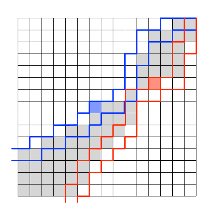
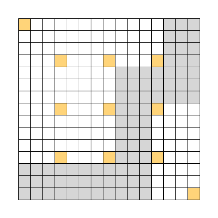
(a)	(b)

Figure 2: Illustrations of tripartitions defined by two contours in a $[15]\times[15]$ grid. Left: the blue and red locations are in $P$. Two possible contours are indicated by blue and red paths. They define a tripartition $(R,S,T)$ with $S$ marked in gray. Right: $P$ is chosen to include two corner locations and an evenly spaced $q\times q$ grid. Any tripartition $(R,S,T)$ defined by a legal pair of contours has $P\cap S=\emptyset$, implying that $|S|\leq 2g^{2}/(q+1)$. An example of an $S$ nearly achieving that size is marked in gray.

5.3 A Randomized Parameterization of the Algorithm

Throughout let $\delta>0$ be a sufficiently small constant. In the randomized implementation of our algorithm we choose $g=s=\delta\ln n/\ln\ln n$ and $p=2+3\delta\ln n$. The points $(0,0)$ and $(g-1,g-1)$ must be in $P$ and the remaining $3\delta\ln n$ points are chosen uniformly at random. With these parameters the probability of a box being bad is sufficiently low to keep the expected cost per search $O(\log g)$.

Lemma 5.1.

The probability a particular box is bad is at most $1/g$.

Proof.

Let $\pi$ be the sorted order for some box $A_{i,j}$. The probability $A_{i,j}$ is bad is precisely the probability that there are $s+1$ consecutive elements (according to $\pi$) that are not included in $P$. The probability that this occurs for a particular set of $s+1$ elements is less than $(1-(p-2)/g^{2})^{s+1}<e^{-(p-2)(s+1)/g^{2}}<e^{-3\ln\ln n}<1/g^{3}$. By a union bound over all $g^{2}-(s+1)$ sets of $s+1$ consecutive elements, the probability $A_{i,j}$ is bad is at most $1/g$. ∎

The expected time per search is therefore $O(\log g)+1/g\cdot O(g)=O(\log g)$. By linearity of expectation the expected total running time is $O(p(n/g)^{2}+n^{2}(\log g)/g)=O(n^{2}(\log\log n)^{2}/\log n)$.

Remark 5.2.

We could have set the parameters differently and achieved the same running time. For example, setting $g=p=\Theta(\log n/\log\log n)$ and $s=\Theta(\log n)$ would also work. The advantage of keeping $s=O(\log n/\log\log n)$ is simplicity: we can afford to enumerate all $s!$ permutations of $S\subset[g]^{2}$ rather than explicitly construct a hyperplane arrangement in order to enumerate only those realizable permutations of $S$.

High Probability Bounds.

The running time of the algorithm may deviate from its expectation with non-negligible probability since the badness events for the boxes $\{A_{i,j}\}$ can be strongly positively correlated. The easiest way to obtain high probability bounds is simply to choose $L=c\log n$ random point sets $\{P_{l}\}_{l\in[L]}$, estimate the cost of the algorithm under each point set, then execute the algorithm under the point set with the best estimated cost. The first step is to run a truncated version of the algorithm in order to determine which queries will be asked in Step 4.2.1. Rather than answer the query $-A(k)\in A_{i,j}$ we simply record the triple $(k,i,j)$ in a list $\mathcal{Q}$ to be answered later. The running time of the algorithm under $P_{l}$ is $O(n^{2}(\log g)/g)$ plus $g$ times the number of bad triples in $\mathcal{Q}$, that is, those $(k,i,j)$ for which $A_{i,j}$ is bad according to $P_{l}$.

Let $\epsilon_{l}$ be the true fraction of bad triples in $\mathcal{Q}$ according to $P_{l}$ and $\hat{\epsilon}_{l}$ be the estimate of $\epsilon_{l}$ obtained by the following procedure. Sample $M=cg^{2}\ln n$ elements of $\mathcal{Q}$ uniformly at random and for each, test whether the given block is bad according to $P_{l}$ by sorting its elements, in $O(g^{2}\log g)$ time. If $X$ is the number of blocks discovered to be bad, report the estimate $\hat{\epsilon}_{l}=X/M$. By a standard version of the Chernoff bound we have

$$\Pr(|\hat{\epsilon}_{l}-\epsilon_{l}|>1/g)=\Pr(|X-{\mathbb{E}\/}(X)|>M/g)<2e^{-2(M/g)^{2}/M}=2n^{-2c}.$$

By Lemma 5.1, ${\mathbb{E}\/}(\epsilon_{l})=1/g$ for each $l$, so by Markov’s inequality $\Pr(\min_{l\in L}\{\epsilon_{l}\}\leq 2/g)\geq 1-2^{-L}=1-n^{-c}$. With high probability, each $\hat{\epsilon}_{l}$ deviates from $\epsilon_{l}$ by at most $1/g$, so the running time of the algorithm will be within a constant factor of its expectation with probability $1-O(n^{-c})$. The time to pick the best point set $P_{l^{\star}}$, $l^{\star}$ being $\operatornamewithlimits{argmin}_{l\in[L]}\{\hat{\epsilon}_{l}\}$, is $O(LMg^{2}\log g)=o(\log^{6}n)$. We could set $L$ and $M$ as high as $n/\operatorname{polylog}(n)$, making the probability that the algorithm deviates from its expectation exponentially small, $\exp(-n/\operatorname{polylog}(n))$.

5.4 A Deterministic Parameterization of the Algorithm

We achieve a subquadratic worst-case 3SUM algorithm by choosing $g,s,p,$ and $P$ such that no block can be bad. Fix $g=(\delta\log n)^{2/3}(\log\log n)^{1/3}$ and $p=2+q^{2}<(\delta\log n)^{2/3}(\log\log n)^{4/3}$ for an integer $q$ to be determined. Aside from the two obligatory points, $P$ contains an evenly spaced $q\times q$ grid in $[g]\times[g]$. Setting $\Delta=\lceil\frac{g+1}{q+1}\rceil$, $P$ is defined as

$$P=\{(0,0),(g-1,g-1)\}\cup\{(k\Delta-1,l\Delta-1)\;|\;\mbox{ where $1\leq k,l\leq q$}\}.$$

See Figure 2(b).

We now argue that no box can be bad if $s=2g(\Delta-1)$. For any legal pair of contours $(\tau,\tau^{\prime})$, in the corresponding tripartition $(R,S,T)$ no element of $P$ can be contained in $S$, that is, in any row (or column) containing elements of $P$, the width (or height) of the band $S$ is at most $\Delta-1$. Since both $\tau$ and $\tau^{\prime}$ are monotone paths in $[g]^{2}$ (non-decreasing by row, non-increasing by column), we always have $|S|<2g(\Delta-1)<2g^{2}/(q+1)<2\delta\log n$. See Figure 2(b) for a worst-case example. For $\delta$ sufficiently small the overhead for reporting dominating pairs will be negligible. The overall running time is therefore $O(n^{2}(\log g)/g)=O(n^{2}/(\log n/\log\log n)^{2/3})$.

6 Linear Degeneracy Testing

Recall that we are given a set $S\subset\mathbb{R}$ and a function $\phi(x_{1},\ldots,x_{k})=\alpha_{0}+\sum_{i=1}^{k}\alpha_{i}x_{i}$, for some real coefficients $\{\alpha_{i}\}$. The problem is to determine if there is a point $(x_{1},\ldots,x_{k})\in S^{k}$ where $\phi$ is zero. As we show below, our 3SUM decision tree can be generalized in a straightforward way to solve $k$-LDT with $O(n^{k/2}\sqrt{\log n})$ comparisons, when $k\geq 3$ is odd. Unfortunately, we do not see how to generalize our 3SUM algorithms to solve $k$-LDT in $O(n^{(k+1)/2}/\operatorname{polylog}(n))$ time, for any odd $k\geq 5$.

Proof.

(of Theorem 1.2) Define $\alpha\cdot S$ to be the set $\{\alpha\cdot a\;|\;a\in S\}$, where $\alpha\in\mathbb{R}$. Begin by sorting the sets

$$A =\{\alpha_{0}+a_{1}+a_{2}+\cdots+a_{(k-1)/2}\;|\;\mbox{$a_{i}\in\alpha_{i}\cdot S$, for each $i>0$}\}$$

and

$$B =\{a_{(k+1)/2}+\cdots+a_{k-1}\;|\;\mbox{$a_{i}\in\alpha_{i}\cdot S$, for each $i$}\}$$

We have effectively reduced $k$-LDT to an unbalanced 3SUM problem. Letting $C$ be the set $\alpha_{k}\cdot S$, the problem is to determine if there exist $a\in A,b\in B,c\in C$ such that $a+b+c=0$. Note that $|A|=|B|=n^{(k-1)/2}$ whereas $|C|=n$. The standard 3SUM algorithm of Section 3 performs $|C|\cdot(|A|+|B|)=n^{(k+1)/2}$ comparisons. Generalizing the decision tree of Section 4 (from one list to three) we can solve unbalanced 3SUM using $O(g(|A|+|B|)+g^{-1}|C|(|A|+|B|)\log g)$ comparisons, which is $O(n^{k/2}\sqrt{\log n})$ when $g=\sqrt{n\log n}$. ∎

Our subquadratic 3SUM algorithms do not extend naturally to unbalanced instances. When $g=\operatorname{polylog}(n)$ we can no longer afford to explicitly sort all $g\times g$ boxes in $A+B$ as this would require at least $\Omega(|A|\cdot|B|/g^{2})=\Omega(n^{k-1}/\operatorname{polylog}(n))$ time.

7 Zero Triangles

We consider a matrix product called target-min-plus that subsumes the $(\min,+)$-product (aka distance product) and the ZeroTriangle problem of [38]. Given real matrices $A\in(\mathbb{R}\cup\{\infty\})^{r\times s},B\in(\mathbb{R}\cup\{\infty\})^{s\times t},$ and a target matrix $T\in(\mathbb{R}\cup\{-\infty,\infty\})^{r\times t}$, the goal is to compute $C=\ocirc(A,B,T)$, where

$$C(i,j)=\min\left\{\,A(i,k)+B(k,j)\>|\>k\in[s]\mbox{ and }A(i,k)+B(k,j)\geq T(i,j)\,\right\}$$

as well as the matrix of witnesses, that is, the $k$ (if any) for which $C(i,j)=A(i,k)+B(k,j)$. This operation reverts to the $(\min,+)$-product when $T(i,j)=-\infty$. It can also solve ZeroTriangle on a weighted graph $G=(V,E,w)$ by setting $A,B,$ and $T$ as follows. Let $A(i,j)=B(i,j)=w(i,j)$, where $w(i,j)\stackrel{{\scriptstyle\operatorname{def}}}{{=}}\infty$ if $(i,j)\not\in E$, and let $T(i,j)=-w(i,j)$ if $(i,j)\in E$ and $\infty$ otherwise. If $C(i,j)=T(i,j)$ then there is a zero weight triangle containing $(i,j)$ and the witness matrix gives the third corner of the triangle.

The trivial target-min-plus algorithm runs in $O(rst)$ time and performs the same number of comparisons. We can compute the target-min-plus product using fewer comparisons using Fredman’s trick.

Theorem 7.1.

The decision-tree complexity of the target-min-plus product of three $n\times n$ matrices is $O(n^{5/2}\sqrt{\log n})$. This product can be computed in $O(n^{3}(\log\log n)^{2}/\log n)$ time.

Proof.

We first show that the target-min-plus product $\ocirc(A,B,T)$ can be determined with $O((r+t)s^{2}+rt\log s)$ comparisons, where $A,B,$ and $T$ are $r\times s,s\times t,$ and $r\times t$ matrices, respectively. Begin by sorting the set

$$D=\{A(i,k)-A(i,k^{\prime}),\>B(k^{\prime},j)-B(k,j)\;|\;i\in[r],j\in[t],\mbox{ and }k,k^{\prime}\in[s]\}.$$

By Lemma 2.3 the number of comparisons required to sort $D$ is $O(|D|+(r+t)s\log(rst))=O((r+t)s^{2}+(r+t)s\log(rst))$. We can now deduce the sorted order on

$$S(i,j)=\{A(i,k)+B(k,j)\;|\;k\in[s]\},$$

for any pair $(i,j)\in[r]\times[t]$, and can therefore find $C(i,j)=\min(S(i,j)\cap[T(i,j),\infty))$ with a binary search over $S(i,j)$ using $\log s$ additional comparisons. The total number of comparisons is $O((r+t)s^{2}+rt\log s)$. Note that this provides no improvement when $A$ and $B$ are square, that is, when $r=s=t=n$. Following Fredman [24] we partition $A$ and $B$ into rectangular matrices and compute their target-min-plus products separately.

Choose a parameter $g$ and partition $A$ into $A_{0},\ldots,A_{\lceil n/g\rceil-1}$ and $B$ into $B_{0},\ldots,B_{\lceil n/g\rceil-1}$ where $A_{\ell}$ contains columns $\ell g,\ldots,(\ell+1)g-1$ of $A$ and $B_{\ell}$ contains the corresponding rows of $B$. For each $\ell\in[n/g]$, compute the target-min-plus product $C_{\ell}=\ocirc(A_{\ell},B_{\ell},T)$ and set $C(i,j)=\min_{\ell\in[n/g]}(C_{\ell}(i,j))$. This algorithm performs $O((n/g)\cdot(ng^{2}+n^{2}\log n))$ comparisons to compute $\{C_{\ell}\}_{\ell\in[n/g]}$ and $n^{2}(n/g)$ comparisons to compute $C$. When $g=\sqrt{n\log n}$ the number of comparisons is $O(n^{5/2}\sqrt{\log n})$.

To compute the product efficiently we use the geometric dominance approach of Chan [15] and Bremner et al. [12]. Choose a parameter $g=\Theta(\log n/\log\log n)$ and partition $A$ into $n\times g$ matrices $\{A_{\ell}\}$ and $B$ into $g\times n$ matrices $\{B_{\ell}\}$. For each $\ell\in[n/g]$ and permutation $\pi:[g]\rightarrow[g]$ we will find those pairs $(i,j)\in[n]^{2}$ for which $\pi$ is the sorted order on $\{A_{\ell}(i,k)+B_{\ell}(k,j)\;|\;k\in[g]\}$. Such a triple satisfies the inequality $A_{\ell}(i,\pi(k))+B_{\ell}(\pi(k),j)<A_{\ell}(i,\pi(k+1))+B_{\ell}(\pi(k+1),j)$, for all $k\in[g-1]$. By Fredman’s trick this is equivalent to saying that the (red) point

$$\left(\ldots,A_{\ell}(i,\pi(k+1))-A_{\ell}(i,\pi(k)),\ldots\right)$$

dominates the (blue) point

$$\left(\ldots,B_{\ell}(\pi(k),j)-B_{\ell}(\pi(k+1),j),\ldots\right)$$

in each of the $g-1$ coordinates. By Lemma 2.5 the total time for all $\lceil n/g\rceil\cdot g!$ invocations of the dominance algorithm is $O((n/g)\cdot g!\cdot c_{\epsilon}^{g-1}(2n/g)^{1+\epsilon})$ plus the output size, which is precisely $n^{2}\lceil n/g\rceil$. For $\epsilon=1/2$ and $g=\Theta(\log n/\log\log n)$ the running time is $O(n^{3}/g)$. We can now compute the target-min-plus product $C_{\ell}=\ocirc(A_{\ell},B_{\ell},T)$ in $O(n^{2}\log g)$ time by iterating over all $(i,j)\in[n]^{2}$ and performing a binary search to find the minimum element in $\{A_{\ell}(i,k)+B_{\ell}(k,j)\;|\;k\in[g]\}\cap[T(i,j),\infty)$. Since $C=\ocirc(A,B,T)$ contains the pointwise minima of $\{C_{\ell}\}$, the total time to compute the target-min-plus product is $O(n^{3}(\log g)/g)=O(n^{3}(\log\log n)^{2}/\log n)$. ∎

The $\sqrt{\log n}$ factor in the decision tree complexity of target-min-plus arises comes from the binary searches, $n/g$ searches per pair $(i,j)\in[n]^{2}$. If the searches were sufficiently correlated (either for fixed $(i,j)$ or fixed $\ell$) then there would be some hope that we could evade the information theoretic lower bound of $\Omega(\log g)$ per search. Using random sampling we form a hierarchy of rectangular target-min-plus products such that the solutions at one level gives a hint for the solutions at the next lower level. The cost of finding the solution, given the hint from the previous level, is $O(1)$ in expectation. The same approach lets us shave off another $\log\log n$ factor off the algorithmic complexity of target-min-plus.

Theorem 7.2.

The randomized decision tree complexity of the target-min-plus product of three $n\times n$ matrices is $O(n^{5/2})$. It can be computed in $O(n^{3}\log\log n/\log n)$ time with high probability.

Proof.

As usual let $A,B,$ and $T$ be $n\times n$ matrices and $g$ be a parameter. We will eventually set $g=\lceil\sqrt{n}\rceil$. We partition the indices $[n]$ at $\log\log n$ levels. Define $I_{l,p}=[pg2^{l},(p+1)g2^{l})$ to be the $p$th interval at level $l$. In other words, level-$l$ intervals have width $g2^{l}$ and a level-$(l+1)$ interval is the union of two level-$l$ intervals. Form a series of nested index sets $[n]=J_{0}\supset J_{1}\supset\cdots\supset J_{\log\log n-1}$, such that $J_{l}\cap I_{l,p}$ is a uniformly random subset of $I_{l,p}$ of size $g$. In other words, each element of $J_{l-1}$ is promoted to $J_{l}$ with probability 1/2, but in such a way that $|J_{l}\cap I_{l,p}|$ is precisely its expectation $g$.

After generating the sets $\{J_{l}\}$ the algorithm sorts $D$ with $O(n^{2}\log n+|D|)=O(n^{5/2})$ comparisons (see Lemma 2.3), where

$$D=\left\{A(i,k)-A(i,k^{\prime}),\;\;B(k^{\prime},i)-B(k,i)\;\;\left|\;\;\begin{array}[]{l}\mbox{$i\in[n]$ and $k,k^{\prime}\in J_{l}\cap I_{l,p}$,}\\ \mbox{for some level $l$ and index $p$}\end{array}\right.\right\}$$

Fix $i,j\in[n]$. We proceed to compute $C(i,j)$ with $O(n/g)$ comparisons with high probability. If $K\subset[n]$ is a set of indices, define $\kappa(K)$ to be the witness of the target-min-plus product restricted to $K$, that is,

$$\kappa(K)=\operatornamewithlimits{argmin}_{\begin{subarray}{c}k\in K\>\text{such that\rule[-2.84526pt]{0.0pt}{2.84526pt}\rule{0.0pt}{7.11317pt}}\\ A(i,k)+B(k,j)\geq T(i,j)\end{subarray}}(A(i,k)+B(k,j)).$$

There may, in fact, be no such witness, in which case $\kappa(K)=\,\perp$. Let $\kappa_{l,p}$ be short for $\kappa(J_{l}\cap I_{l,p})$. Notice that by Fredman’s trick we can deduce the sorted order on

$$S_{l,p}=\{A(i,k)+B(k,j)\;|\;k\in J_{l}\cap I_{l,p}\}$$

without additional comparisons, for any $l$ and $p$. We can therefore compute the top-level witnesses $\{\kappa_{\log\log n-1,p}\}_{p\in[n/(g2^{\log\log n-1})]}$ with $O(\frac{n}{g2^{\log\log n}}\cdot\log n)=O(\sqrt{n})$ comparisons via binary search. Our goal now is to compute the witnesses at all lower level intervals with $O(\sqrt{n})$ comparisons. Suppose we have computed the level-$(l+1)$ witness $\kappa_{l+1,p}$ and wish to compute the level-$l$ witnesses of the constituent sequences, namely $\kappa_{l,2p}$ and $\kappa_{l,2p+1}$. Define $\kappa_{l,2p}^{\prime}=\kappa(J_{l+1}\cap I_{l,2p})$. Note that $\kappa_{l,2p}^{\prime}$ is determined by $\kappa_{l+1,p}$ and the sorted order on $S_{l+1,p}$. The distance between $\kappa_{l,2p}$ and $\kappa_{l,2p}^{\prime}$ (according to the sorted order on $S_{l,2p}$) is stochastically dominated by a geometric random variable with mean 1. The expected number of comparisons needed to determine $\kappa_{l,p}$ using linear search is therefore $O(1)$. These geometric random variables are independent due to the independence of the samples, so we can apply standard Chernoff-type concentration bounds [19]. The probability that the sum of these independent geometric random variables exceeds twice its expectation $\mu$ is $\exp(-\Omega(\mu))=\exp(-\Omega(\sqrt{n}))$.

Once we have computed all the witnesses for level-0, $\{\kappa_{0,p}\}_{p\in[n/g]}$, we simply have to choose the best among them, so $C(i,j)=\min\{A(i,\kappa_{0,p})+B(\kappa_{0,p},j)\;|\;p\in[n/g]\mbox{ and }\kappa_{0,p}\neq\perp\}$. The total number of witnesses computed for fixed $i,j$ is $\sum_{l\geq 0}n/(g2^{l})<2n/g$. The total number of comparisons is therefore $O(n^{2}g)$ to sort $D$ and $O(n^{3}/g)$ to compute all the witnesses and $C$, which is $O(n^{5/2})$ when $g=\sqrt{n}$.

To improve the $O(n^{3}(\log\log n)^{2}/\log n)$ algorithm we apply the ideas above with different parameters. Let $g=\Theta(\log n/\log\log n)$. We consider the same partitions $\{I_{l,p}\}_{l,p}$ and nested index sets $\{J_{l}\}_{l}$, but only use the first $\log\log\log n$ levels, not $\log\log n$ as before. For each level $l\in[\log\log\log n]$, index $p\in[n/(g2^{l})]$, and permutation $\pi\,:\,[g]\rightarrow[g]$, we compute those pairs $(i,j)$ for which $\pi$ is the sorting permutation on the elements of $J_{l}\cap I_{l,p}$. This can be done in time linear in the output size, at most $2n^{3}/g$, and $\sum_{l\in[\log\log\log n]}\frac{n}{g2^{l}}g!c_{\epsilon}n^{1+\epsilon}$. When $\epsilon=1/2$ and $g$ is sufficiently small the time spent computing dominating pairs is $O(n^{3}/g)$. Since $g=\Theta(\log n/\log\log n)$ we can encode the sorting permutation of each $J_{l}\cap I_{l,p}$ in one word and can answer a variety of queries about these permutations in $O(1)$ time using $O(n)$-size precomputed tables.

Fix a pair $(i,j)\in[n]^{2}$. When finding the top-level witnesses $\{\kappa_{\log\log\log n-1,p}\}_{p\in[2n/(g\log\log n)]}$ we can implement each step of the binary searches in $O(1)$ time using table lookups, for a total of $O(n/g)$ time. We can also implement each step of the linear searches for witnesses $\kappa_{l,2p}$ and $\kappa_{l,2p+1}$ in $O(1)$ time using table lookups. (In addition to encoding the sorting permutations on $J_{l+1}\cap I_{l+1,p}$, $J_{l}\cap I_{l,2p}$, and $J_{l}\cap I_{l,2p+1}$, we also need to encode the positions of $J_{l+1}\cap I_{l+1,p}$ within $J_{l}\cap I_{l+1,p}$ as a length-$2g$ bit vector. This is needed in order to find $\kappa_{l,2p}^{\prime}$ and $\kappa_{l,2p+1}^{\prime}$ in $O(1)$ time, given $\kappa_{l+1,p}$ and the sorted order on $S_{l+1,p}$.) Over all $(i,j)\in[n]^{2}$ the total number of comparisons is $O(n^{3}/g)=O(n^{3}\log\log n/\log n)$ with high probability. ∎

The trivial time to solve ZeroTriangle on sparse $m$-edge graphs is $O(m^{3/2})$. Such graphs contain at most $O(m^{3/2})$ triangles, which can be enumerated in $O(m^{3/2})$ time. We now restate and prove 1.4.

Theorem 1.4. The decision tree complexity of ZeroTriangle on $m$-edge graphs is $O(m^{5/4}\sqrt{\log m})$ and, using randomization, $O(m^{5/4})$ with high probability. The ZeroTriangle problem can be solved in $O(m^{3/2}(\log\log m)^{2}/\log m)$ time deterministically or $O(m^{3/2}\log\log m/\log m)$ with high probability.  

Proof.

We begin by greedily finding an acyclic orientation of the graph $G=(V,E,w)$. Iteratively choose the vertex $v$ with the fewest number of still unoriented edges and direct them all away from $v$. Since every $m$-edge graph contains a vertex of degree less than $\Delta=\sqrt{2m}$, the maximum outdegree in this orientation is less than $\Delta$. We now use $\vec{E}$ instead of $E$ to emphasize that the set is oriented.

Select a random mapping $\mbox{\sc color}:V\rightarrow[K]$, where $K$ will be fixed soon. The expected number of pairs of oriented edges $\{(u,x),(u,x^{\prime})\}\subset\vec{E}$ having $\mbox{\sc color}(x)=\mbox{\sc color}(x^{\prime})$ is less than $m\Delta/K$. Any coloring that does not exceed this expected value suffices; we do not need to choose color at random. We now sort the set $D$ with $O(m\log m+|D|)=O(m\log m+m\Delta/K)$ comparisons [23], where

$$D=\{w(u,x)-w(u,x^{\prime})\;\,|\,\;u\in V\,\mbox{ and }\,(u,x),(u,x^{\prime})\in\vec{E}\,\mbox{ and }\,\mbox{\sc color}(x)=\mbox{\sc color}(x^{\prime})\}.$$

Call a triangle on $\{u,v,x\}$ type-$((u,v),\kappa)$ if the orientation of the edges is $(u,v),(u,x),(v,x)$ and $\mbox{\sc color}(x)=\kappa$. Clearly every triangle is of one type and there are $mK$ types. A type-$((u,v),\kappa)$ zero-weight triangle exists iff $-w(u,v)$ appears in the set $\{w(u,x)+w(v,x)\;|\;\mbox{$x\in V$ and $\mbox{\sc color}(x)=\kappa$}\}$. By Fredman’s trick the sorted order of this set is determined by the sorted order of $D$, since $w(u,x)+w(v,x)<w(u,x^{\prime})+w(v,x^{\prime})$ iff $w(u,x)-w(u,x^{\prime})<w(v,x^{\prime})-w(v,x)$. See Figure 3. We can therefore determine if there exists a zero-weight triangle of a particular type with $O(\log\Delta)$ comparisons via binary search. The total number of comparisons is $O(m\log m+m\Delta/K+mK\log\Delta)$, which is $O(m^{5/4}\sqrt{\log m})$ when $K=\sqrt{\Delta/\log\Delta}=O(m^{1/4}/\sqrt{\log m})$. The $\sqrt{\log m}$ factor can be shaved off using randomization, exactly as in Theorem 7.2. We form $\log\log n$ levels of colorings, where color class $p$ at the $(l+1)$th level is the union of classes $2p$ and $2p+1$ at the $l$th level. After the searches are conducted at level $l+1$, the expected cost per search at level $l$ is $O(1)$.

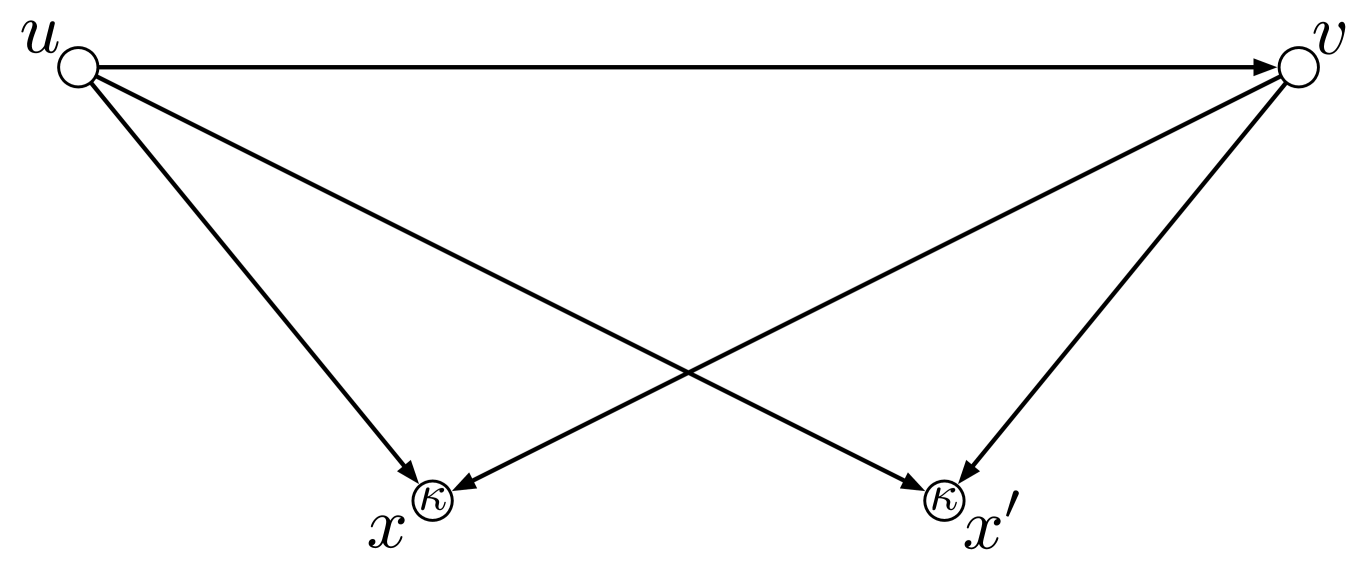
Figure 3: In this example $\mbox{\sc color}(x)=\mbox{\sc color}(x^{\prime})=\kappa$ and both triangles on $\{u,v,x\}$ and $\{u,v,x^{\prime}\}$ are of the same type.

To solve ZeroTriangle efficiently we greedily orient the graph as before, stopping when all remaining vertices have degree at least $\Delta$, where $\Delta$ is a parameter to be fixed shortly. (The unoriented subgraph remaining is called the $\Delta$-core.) For each vertex $u$ and each pair of outgoing edges $(u,v),(u,x)\in\vec{E}$, we check whether $(u,v,x)$ is a triangle and, if so, whether it has zero weight. (Note that the edge $(v,x)$, if it exists, may be in the $\Delta$-core and therefore not have an orientation.) This takes $O(m\Delta)$ time. It remains to check triangles contained entirely in the $\Delta$-core. Since the $\Delta$-core has at most $2m/\Delta$ vertices we can solve ZeroTriangle on it in $O((m/\Delta)^{3}(\log\log m)^{2}/\log m)$ time or $O((m/\Delta)^{3}\log\log m/\log m)$ time with high probability. The total cost is balanced when $\Delta=\sqrt{m}\left((\log\log m)^{2}/\log m)\right)^{1/4}$ or $\Delta=\sqrt{m}\left(\log\log m/\log m\right)^{1/4}$ depending on whether uses the randomized or deterministic ZeroTriangle algorithm. ∎

The Convolution3SUM problem is easily reducible to 3SUM, so our $O(n^{3/2}\sqrt{\log n})$ and $O(n^{2}/\operatorname{polylog}(n))$ bounds for 3SUM extend directly to Convolution3SUM. However, Convolution3SUM has additional structure, which makes it amenable to the same random sampling techniques used in Theorem 7.2. We give only a sketch of the proof of Theorem 1.5 as the analysis is essentially the same as that found in Theorem 7.2.

Theorem 1.5. The decision tree complexity of Convolution3SUM is $O(n^{3/2}\sqrt{\log n})$ and its randomized decision tree complexity is $O(n^{3/2})$ with high probability. The Convolution3SUM problem can be solved in $O(n^{2}(\log\log n)^{2}/\log n)$ time deterministically, or in $O(n^{2}\log\log n/\log n)$ time with high probability.  

Proof.

(sketch) In the Convolution3SUM problem we must determine if there is a $k\in[n]$ such that $A(k)$ occurs on the $k$th antidiagonal of the matrix $A+A$. In contrast to 3SUM, the rows and columns of $A+A$ are not sorted. On the other hand, we do not need to look for $A(k)$ in the whole matrix, just those locations along an antidiagonal.

The $O(n^{3/2}\sqrt{\log n})$ decision tree bound is proved as in Section 4, by partitioning the matrix into $g\times g$ blocks and for each $k$, conducting binary searches for $A(k)$ in the appropriate antidiagonals of at most $2n/g$ boxes. In order to shave off the $\sqrt{\log n}$ factor we use the same random sampling approach of Theorem 7.2. We partition $A+A$ at $\log\log n$ levels, where level-$l$ boxes have size $g2^{l}\times g2^{l}$ and are the union of four level-$(l-1)$ boxes. The rows and columns are sampled at $\log\log n$ levels, where a row or column at level $l-1$ is promoted to level $l$ with probability 1/2. Note that an element of $A+A$ appears at level-$l$ if and only if both its row and column are in the level-$l$ sample. Since elements along any antidiagonal share no rows or columns, the events that they appear at level-$l$ are entirely independent. This independence property allows us to search for $A(k)$ in level-$l$ sampled boxes in $O(1)$ expected time, given the predecessors of $A(k)$ in the level-$(l+1)$ sampled boxes. Algorithms running in $O(n^{2}(\log\log n)^{2}/\log n)$ (deterministically) or $O(n^{2}\log\log n/\log n)$ (with high probability) are obtained using the methods applied in Theorems 7.1 and 7.2. Alternatively, we could apply the Williams-Williams reduction [38] from Convolution3SUM to ZeroTriangle and then invoke the algorithms of Theorems 7.1 and 7.2 as black boxes. ∎

8 Conclusion

Since the introduction of Fredman’s [23] $(\min,+)$-product algorithm in 1976, many have become comfortable with the idea that some numerical problems naturally have a large gap ($\tilde{\Omega}(\sqrt{n})$) between their (nonuniform) decision-tree complexity and (uniform) algorithmic complexity. From this perspective, our decision trees for 3SUM and ZeroTriangle (with depth $\tilde{O}(n^{3/2}$ and $\tilde{O}(n^{5/2})$) do not constitute convincing evidence that 3SUM and ZeroTriangle have truly subquadratic and subcubic algorithms. However, Williams’s [36] recent breakthrough on the algorithmic complexity of $(\min,+)$-product should shake one’s confidence that these $\sqrt{n}$ gaps are natural. To close them one may simply need to develop more sophisticated algorithmic machinery.

The exponent $3/2$ has a special significance in Pǎtraşcu’s program [32] of conditional lower bounds based on hardness of 3SUM. His superlinear lower bounds on triangle enumeration and polynomial lower bounds on dynamic data structures depend on the complexity of 3SUM being $\Omega(n^{3/2+\epsilon})$, for some $\epsilon>0$. In most other 3SUM-hardness proofs there is nothing sacred about the 3/2 threshold (or any other exponent). For example, if 3SUM requires $\Omega(n^{1.05})$ time then finding three collinear points in a set $P\subset\mathbb{R}^{2}$ also requires $\Omega(|P|^{1.05})$ time [25].

Appendix A Bichromatic Dominating Pairs

For the sake of completeness we shall review a standard divide and conquer dominating pairs algorithm of Preparata and Shamos [31, p. 366] and give a short proof of Lemma 2.5 due to Chan [15].

A.1 The Divide and Conquer Algorithm

We are given $n$ red and blue points in $P\subset\mathbb{R}^{d}$, at least one of each color, and wish to report all pairs $(p,q)$ where $p=(p_{i})_{i\in[d]}$ is red, $q=(q_{i})_{i\in[d]}$ is blue and $p_{i}\geq q_{i}$ for each $i\in[d]$. When $d=0$ the algorithm simply reports every pair of points, so assume $d\geq 1$. Find the median $h$ on the last coordinate in $O(n)$ time [11] and partition $P$ into disjoint sets $P_{L}$, $P_{R}$ of size at most $\lceil n/2\rceil$, where

$$P_{L} \subset\{p\in P\>|\>p_{d-1}\leq h\}$$

$$P_{R} \subset\{p\in P\>|\>p_{d-1}\geq h\}.$$

Furthermore, there cannot be a red $p\in P_{L}$ and blue $q\in P_{R}$ such that $p_{d-1}=q_{d-1}=h$. At this point all dominating pairs are in $P_{L},$ or $P_{R}$, or have one point in each, in which case the blue point is necessarily in $P_{L}$ and the red in $P_{R}$. We make three recursive calls to find dominating pairs of each variety. The first two calls are on $\lceil n/2\rceil$ points in $\mathbb{R}^{d}$. The third recursive call is on all blue points in $P_{L}$ and all red points in $P_{R}$; after stripping their last coordinate they lie in $\mathbb{R}^{d-1}$.

Excluding the cost of reporting the output, the running time of this algorithm is bounded by $T_{d}(n)$, defined inductively as

$$T_{0}(n) =T_{d}(1)\,=\,0$$

$$T_{d}(n) =2T_{d}(n/2)+T_{d-1}(n)+n$$

We prove by induction that $T_{d}(n)\leq c_{\epsilon}n^{1+\epsilon}-n$, a bound which holds in all base cases. Assuming the claim holds for all smaller values of $d$ and $n$,

$$T_{d}(n) \leq 2\left(c_{\epsilon}^{d}(n/2)^{1+\epsilon}-n/2\right)+\left(c_{\epsilon}^{d-1}n^{1+\epsilon}-n\right)+n$$

$$=\left(c_{\epsilon}^{d}/2^{\epsilon}+c_{\epsilon}^{d-1}\right)n^{1+\epsilon}-n$$

$$=\left(1/2^{\epsilon}+1/c_{\epsilon}\right)\cdot c_{\epsilon}^{d}n^{1+\epsilon}-n$$

$$=c_{\epsilon}^{d}n^{1+\epsilon}-n c_{\epsilon}=2^{\epsilon}/(2^{\epsilon}-1)$$ By defn. of .

References

- [1] O. Weimann A. Abboud, V. Vassilevska Williams. Consequences of faster sequence alignment. In Proceedings 41st Int’l Colloquium on Automata, Languages, and Programming (ICALP), page ?, 2014.
- [2] A. Abboud and K. Lewi. Exact weight subgraphs and the -sum conjecture. In Proceedings of the 40th Int’l Colloquium on Automata, Languages, and Programming (ICALP), pages 1–12, 2013.
- [3] A. Abboud and V. Vassilevska Williams. Popular conjectures imply strong lower bounds for dynamic problems. CoRR, abs/1402.0054, 2014.
- [4] O. Aichholzer, F. Aurenhammer, E. D. Demaine, F. Hurtado, P. Ramos, and J. Urrutia. On -convex polygons. Comput. Geom., 45(3):73–87, 2012.
- [5] N. Ailon and B. Chazelle. Lower bounds for linear degeneracy testing. J. ACM, 52(2):157–171, 2005.
- [6] A. Amir, T. M. Chan, M. Lewenstein, and N. Lewenstein. Consequences of faster sequence alignment. In Proceedings 41st Int’l Colloquium on Automata, Languages, and Programming (ICALP), page ?, 2014.
- [7] R. Bar-Yehuda and S. Fogel. Partitioning a sequence into few monotone subsequences. Acta Informatica, 35:421–440, 1998.
- [8] I. Baran, E. D. Demaine, and M. Pǎtraşcu. Subquadratic algorithms for 3SUM. Algorithmica, 50(4):584–596, 2008.
- [9] G. Barequet and S. Har-Peled. Polygon containment and translational min-Hausdorff-distance between segment sets are 3SUM-hard. Int. J. Comput. Geometry Appl., 11(4):465–474, 2001.
- [10] A. Bjorklund, R. Pagh, V. Vassilevska Williams, and U. Zwick. Listing triangles. In Proceedings 41st Int’l Colloquium on Automata, Languages, and Programming (ICALP), page ?, 2014.
- [11] M. Blum, R. W. Floyd, V. Pratt, R. L. Rivest, and R. E. Tarjan. Time bounds for selection. J. Comput. Syst. Sci., 7(4):448–461, 1973.
- [12] D. Bremner, T. M. Chan, E. D. Demaine, J. Erickson, F. Hurtado, J. Iacono, S. Langerman, M. Pǎtraşcu, and P. Taslakian. Necklaces, convolutions, and X + Y. Algorithmica, 69:294–314, 2014.
- [13] R. C. Buck. Partition of space. Amer. Math. Monthly, 50:541–544, 1943.
- [14] A. Butman, P. Clifford, R. Clifford, M. Jalsenius, N. Lewenstein, B. Porat, E. Porat, and B. Sach. Pattern matching under polynomial transformation. SIAM J. Comput., 42(2):611–633, 2013.
- [15] T. M. Chan. All-pairs shortest paths with real weights in time. Algorithmica, 50(2):236–243, 2008.
- [16] S. Chechik, D. Larkin, L. Roditty, G. Schoenebeck, R. E. Tarjan, and V. Vassilevska Williams. Better approximation algorithms for the graph diameter. In Proceedings of the 25th Annual ACM-SIAM Symposium on Discrete Algorithms (SODA), pages 1041–1052, 2014.
- [17] K.-Y. Chen, P.-H. Hsu, and K.-M. Chao. Approximate matching for run-length encoded strings is 3SUM-hard. In Combinatorial Pattern Matching, volume 5577 of Lecture Notes in Computer Science, pages 168–179. 2009.
- [18] E. W. Dijkstra. Some beatiful arguments using mathematical induction. Acta Informatica, 13:1–8, 1980.
- [19] D. P. Dubhashi and A. Panconesi. Concentration of Measure for the Analysis of Randomized Algorithms. Cambridge University Press, 2009.
- [20] H. Edelsbrunner, J. O’Rourke, and R. Seidel. Constructing arrangements of lines and hyperplanes with applications. SIAM J. Comput., 15(2):341–363, 1986.
- [21] P. Erdös and P. Turán. On a problem of Sidon in additive number theory, and on some related problems. Journal of the London Mathematical Society, 1(4):212–215, 1941.
- [22] J. Erickson. Bounds for linear satisfiability problems. Chicago J. Theor. Comput. Sci., 1999.
- [23] M. L. Fredman. How good is the information theory bound in sorting? Theoretical Computer Science, 1(4):355–361, 1976.
- [24] M. L. Fredman. New bounds on the complexity of the shortest path problem. SIAM J. Comput., 5(1):83–89, 1976.
- [25] A. Gajentaan and M. H. Overmars. On a class of problems in computational geometry. Comput. Geom., 5:165–185, 1995.
- [26] J. Hartmanis and R. E. Stearns. On the computational complexity of algorithms. Trans. Amer. Math. Soc., 117:285–306, 1965.
- [27] Z. Jafargholi and E. Viola. 3SUM, 3XOR, triangles. CoRR, abs/1305.3827, 2013.
- [28] J.-L. Lambert. Sorting the sums in comparisons. Theor. Comput. Sci., 103(1):137–141, 1992.
- [29] S. Meiser. Point location in arrangements of hyperplanes. Information and Computation, 106(2):286–303, 1993.
- [30] F. Meyer auf der Heide. A polynomial linear search algorithm for the -dimensional knapsack problem. J. ACM, 31(3):668–676, 1984.
- [31] F. P. Preparata and M. I. Shamos. Computational Geometry. Springer, New York, NY, 1985.
- [32] M. Pǎtraşcu. Towards polynomial lower bounds for dynamic problems. In Proceedings 42nd ACM Symposium on Theory of Computing (STOC), pages 603–610, 2010.
- [33] M. Pǎtraşcu and R. Williams. On the possibility of faster SAT algorithms. In Proceedings of the 21st Annual ACM-SIAM Symposium on Discrete Algorithms (SODA), pages 1065–1075, 2010.
- [34] L. Roditty and V. Vassilevska Williams. Fast approximation algorithms for the diameter and radius of sparse graphs. In Proceedings 45th ACM Symposium on Theory of Computing (STOC), pages 515–524, 2013.
- [35] M. A. Soss, J. Erickson, and M. H. Overmars. Preprocessing chains for fast dihedral rotations is hard or even impossible. Comput. Geom., 26(3):235–246, 2003.
- [36] R. Williams. Faster all-pairs shortest paths via circuit complexity. In Proceedings of the 46th Annual ACM Symposium on Theory of Computing (STOC), 2014. Technical report available as arXiv:1312.6680.
- [37] V. Vassilevska Williams and R. Williams. Subcubic equivalences between path, matrix and triangle problems. In Proceedings 51th Annual IEEE Symposium on Foundations of Computer Science (FOCS), pages 645–654, 2010.
- [38] V. Vassilevska Williams and R. Williams. Finding, minimizing, and counting weighted subgraphs. SIAM J. Comput., 42(3):831–854, 2013.