Atom-field entanglement in two-atom Jaynes-Cummings model with intensity-dependent coupling

Abstract

An exact solution of the problem of two-atom one- and two-mode Jaynes-Cummings model with intensity-dependent coupling is presented. Asymptotic solutions for system state vectors are obtained in the approximation of large initial coherent fields. The atom-field entanglement is investigated on the basis of the reduced atomic entropy dynamics. The possibility of the system being initially in a pure disentangled state to revive into this state during the evolution process for both models is shown. Conditions and times of disentanglement are derived.

1 Introduction

Entanglement plays a central role in quantum information, quantum computation and communication, and quantum cryptography. In recent years, there has been a considerable effort to characterize entanglement properties qualitatively and quantitatively and to apply them in quantum information. A lot of schemes are proposed for many-particle entanglement generation. The simplest scheme to investigate the atom-field entanglement is the Jaynes-Cummings model (JCM) jc describing an interaction of a two-level atom with a single-mode quantized radiation field. This model is of fundamental importance for quantum optics Yoo ; Shore and is realizable to a very good approximation in experiments with Rydberg atoms in high-Q superconducting cavities, trapped ions, superconducting circuits etc. Walter ; Haroche ; Nori . The model predicts a variety of interesting phenomena. The atom-field entanglement is among them. An investigation of the atom-field entanglement for JCM has been initiated by Phoenix and Knight Knightearly ,Knight and Gea-Banacloche Gea-Banacloche ,Gea-Banacloche1 . Gea-Banacloche has derived an asymptotic result for the JCM state vector which is valid when the field is initially in a coherent state with a large mean photon number. It is shown that the atom prepared in arbitrary initial pure atomic state is to a good approximation in a pure state in the middle of the collapse region. This has been first noticed by Phoenix and Knight by using the entropy concepts. An appreciable disentanglement between atom and field is found at the half-revival time, otherwise the atom and field are strongly entangled. Moreover, at the half-revival time, the cavity field represents a coherent superposition of the two macroscopically distinct states with opposite phases or so-called Schr$\ddot{\rm o}$edinger cat state. The theory outlined in Gea-Banacloche has been generalized for two-photon JCM Dung1 ,Nasreen , two-photon JCM with nondegenerate two-photon and Raman transitions Abdalla ,Larson , two-atom JCM Kudryavtsev , Dung , two-atom one-mode Raman coupled model Rdegen and two-atom two-photon JCM bash1 -bash3 .

Two-photon processes are known to play a very important role in atomic systems due to high degree of correlation between emitted photons. An interest for investigation of the two-photon JCM is stimulated by the experimental realization of a two-photon one-atom micromaser on Rydberg transitions in a microwave cavity Brune . A nondegenerate two-photon two-mode maser, which represents a two-level Rydberg atom interacting with two different modes of a quantum electromagnetic field in a high-quality cavity through a nondegenerate two-photon transition, is an important generalization of the model of a two-photon micromaser. A possibility of the modulation, amplification and control of one mode with another mode is an important feature of the two-photon two-mode maser. JCM with nondegenerate two-photon transitions have attracted a great deal of attention. The foregoing model have been considered in terms of atomic population dynamics research, field statistics research, field and atom squeezing analysis, atom and field entropy and entanglement examining Del . The two-atom two-photon JCM for initial two-mode coherent cavity field has been investigated for nondegenerate two-photon transitions in Bash .

As it was pointed out by Singh and Amrita Singh the Cavity Quantum Electrodynamics (QED) generally deals with few cavity photons, hence, atomic emission and absorption effects are expected to change the atom-field interaction strength significantly. Consequently an intensity-dependent coupling constant would be appropriate to study the problems related to cavity QED. The dynamical properties of the intensity-dependent one- and two-atom JCM for a two-mode cavity field have been investigated recently in Refs Singh -Hekmatara .

In this paper we analyze the atomic and field state evolution and atom-field entanglement in the two-atom one- and two-mode JCM with intensity-dependent coupling, as in Gea-Banacloche1 , that the field is initially in a one- or two-mode coherent state with a large mean photon numbers correspondingly. We study systems by using the linear atomic entropy concepts and the asymptotic behavior of the system state vectors in the approximation of large initial coherent field. The main goal of this paper is to show such initial states of atomic subsystem which provide disentanglement between atom and field at certain times. We also have estimated these disentanglement times. In the framework of large initial field the atomic eigenstates of the semiclassical Hamiltonian are found. It is shown that if atoms are initially prepared in one of these states, the system evolves remaining the atomic and field parts separately disentangled in a pure state. However, only for certain initial atomic states the disentanglement between atom and field occurs.

2 Model description. The exact solution of Schr$\ddot{\rm o}$edinger equation for wave function

We have investigated atom-field entanglement for two type of two-atom JCM with the intensity-dependent coupling. The first of them describes two two-level atoms resonantly interacting with one-mode coherent field in lossless cavity. The interaction Hamiltonian of such a model is

$$H_{int}=\hbar g\sum_{i=1}^{2}\left(\sqrt{a^{+}a}a^{+}\sigma_{i}^{-}+\sigma_{i}^{+}a\sqrt{a^{+}a}\right),$$

Here we use the following notation : $a^{+}\,(a)$ is creation (annihilation) operator for cavity mode, $\sigma_{i}^{+}=|+\rangle_{ii}\langle-|$ and $\sigma_{i}^{-}=|-\rangle_{ii}\langle+|$ are the atomic transition operators, while $|-\rangle_{i}$ and $|+\rangle_{i}$ denote the ground and excited states of the $i$th two-level atom ($i=1,\,2$) respectively. Parameter $g$ with the operator $\sqrt{a^{+}a}$ plays the role of intensity-dependent coupling constant between atoms and the cavity field. The second model describes two two-level atoms interacting with two-mode coherent field in lossless cavity via nondegenerate two-photon transitions under the assumption of exact two-photon resonance. The effective interaction Hamiltonian for considered model can be written in the following form Singh2 :

$$H_{int}=\hbar g\sum^{2}_{i=1}{(\sqrt{a^{+}_{1}a_{1}}a^{+}_{1}\sqrt{a^{+}_{2}a_{2}}a^{+}_{2}\sigma^{-}_{i}+a_{1}\sqrt{a^{+}_{1}a_{1}}{a_{2}\sqrt{a^{+}_{2}a_{2}}\sigma}^{+}_{i})}.$$

In formulae (2) we use the following notations: $a_{j}^{+}\,(a_{j})$ is creation (annihilation) operator for $j$-th cavity mode ($j=1,2)$ and $g$ is the effective constant of dipole-photon interaction. In two-photon processes the Stark shift caused by the intermediate atomic level plays the role of an intensity-dependent detuning. However, if the two fields are tuned in such a way that both have reverse detuning with the intermediate atomic level, the Stark shift will not appear as has been pointed in Ref. Singh2 . Such a two-photon signal could be achieved by two dye lasers.

Atoms are supposed to be initially prepared in arbitrary pure atomic states superposition

$$|\Psi(0)\rangle_{A}=\alpha|+,+\rangle+\beta|+,-\rangle+\gamma|-,+\rangle+\delta|-,-\rangle$$

and field is supposed to be initially in one-mode or two-mode coherent state. The full wave function of atom-field system at initial time for the first model can be written as

$$|\Psi(0)\rangle=|\Psi(0)\rangle_{A}|\upsilon\rangle$$

and for the second model can be written as

$$|\Psi(0)\rangle=|\Psi(0)\rangle_{A}|\upsilon_{1}\upsilon_{2}\rangle.$$

Here $\alpha,\beta,\gamma$ and $\delta$ are arbitrary complex values satisfying the condition

$$|\alpha|^{2}+|\beta|^{2}+|\gamma|^{2}+|\delta|^{2}=1.$$

Here

$$|\upsilon\rangle=\sum_{n=0}^{\infty}F_{n}|n\rangle$$

is one-mode and

$$|\upsilon_{1}\upsilon_{2}\rangle=\sum_{n_{1}=0}^{\infty}\sum_{n_{2}=0}^{\infty}F_{n_{1}}F_{n_{2}}|n_{1}\rangle|n_{2}\rangle\>$$

is two-mode coherent state correspondingly, where the coefficients $F_{n}$ are

$$F_{n}=exp(-\overline{n}/2)\frac{\overline{n}^{n/2}}{\sqrt{n!}}e^{\imath\varphi}\,\>,$$

where $\upsilon=\overline{n}^{1/2}e^{\imath\varphi}$, $\overline{n}=|\upsilon|^{2}$ is the mean photon number and $\varphi$ is the phase of coherent mode.

The exact solution of Shr$\ddot{\rm o}$edinger equation for wave function under considered initial conditions for model with Hamiltonian (1) takes the form of:

$$|\Psi(t)\rangle=\sum_{n}\left[A_{n}(t)|+,+\rangle+B_{n}(t)|+,-\rangle+C_{n}(t)|-,+\rangle+D_{n}(t)|-,-\rangle\right]|n\rangle.$$

Here for one-mode two-atom JCM the following notation is accepted:

$$A_{n}(t) = \frac{(n+2)^{2}+(n+1)^{2}\cos(2\Omega_{n}t)}{2\Omega_{n}^{2}}\alpha F_{n}-\imath\frac{(n+1)\sin(2\Omega_{n})}{2\Omega_{n}}\beta F_{n+1}-$$

$$- \imath\frac{(n+1)\sin(2\Omega_{n}t)}{2\Omega_{n}}\gamma F_{n+1}-\frac{(n+1)(n+2)\sin^{2}(\Omega_{n}t)}{\Omega_{n}^{2}}\delta F_{n+2},$$

$$B_{n}(t) = -\imath\frac{n\sin(2\Omega_{n-1}t)}{2\Omega_{n-1}}\alpha F_{n-1}+\cos^{2}(\Omega_{n-1}t)\beta F_{n}-$$

$$- \sin^{2}(\Omega_{n-1}t)\gamma F_{n}-\imath\frac{(n+1)\sin^{2}(\Omega_{n-1}t)}{2\Omega_{n-1}}\delta F_{n+1},$$

$$C_{n}(t) = -\imath\frac{n\sin(2\Omega_{n-1}t)}{2\Omega_{n-1}}\alpha F_{n-1}-\sin^{2}(\Omega_{n-1}t)\beta F_{n}+$$

$$+ \cos^{2}(\Omega_{n-1}t)\gamma F_{n}-\imath\frac{(n+1)\sin^{2}(\Omega_{n-1}t)}{2\Omega_{n-1}}\delta F_{n+1},$$

$$D_{n}(t) = -\frac{(n-1)n\sin^{2}(\Omega_{n-2}t)}{\Omega_{n-2}^{2}}\alpha F_{n-2}-\imath\frac{n\sin(2\Omega_{n-2}t)}{2\Omega_{n-2}}\beta F_{n-1}-$$

$$- \imath\frac{n\sin(2\Omega_{n-2}t)}{2\Omega_{n-2}}\gamma F_{n-1}+\frac{((n-1)^{2}+n^{2})\cos^{2}(\Omega_{n-2}t)}{2\Omega_{n-2}^{2}}\delta F_{n},$$

where

$$\Omega_{n}=\sqrt{\left[2n(n+3)+5\right]/2}.$$

The exact solution of Shr$\ddot{\rm o}$edinger equation for wave function under considered initial conditions for model with Hamiltonian (2) is

$$|\Psi(t)\rangle=\sum^{\infty}_{n_{1},n_{2}=0}\left[A_{n_{1}n_{2}}(t)|+,+\rangle+B_{n_{1}n_{2}}t)|+,-\rangle+\right.$$

$$\left.+C_{n_{1}n_{2}}(t)|-,+\rangle+D_{n_{1}n_{2}}(t)|-,-\rangle\right)|n_{1},n_{2}\rangle.$$

Here the following notation is accepted:

$$A_{n_{1}n_{2}}\left(t\right) = \frac{2\alpha F_{n_{1}}F_{n_{2}}}{{\Omega}^{2}_{1}}\left(X_{1}\left(n_{1}+1\right)\left(n_{2}+1\right){\cos{\Omega}_{{\rm 1}}{\rm t+}{{\rm X}}_{{\rm 2}}{(n}_{1}+2)(n_{2}+2)\ }\right)+$$

$$+ \frac{2\beta F_{n_{1}+2}F_{n_{2}+2}}{{\Omega}^{2}_{1}}X^{2}_{2}\left(cos{\Omega}_{{\rm 1}}t-1\right)-+$$

$$- i\frac{\left(\gamma+\delta\right)F_{n_{1}+1}F_{n_{2}+1}}{{\Omega}_{{\rm 1}}}\left(n_{1}+1\right)\left(n_{2}+1\right)sin{\Omega}_{{\rm 1}}{\rm t,}$$

$$B_{n_{1}n_{2}}\left(t\right) = -i\frac{\alpha F_{n_{1}-1}F_{n_{2}-1}}{{\Omega}_{3}}X_{3}sin{\Omega}_{{\rm 3}}t-i\frac{\beta F_{n_{1}+1}F_{n_{2}+1}}{{\Omega}_{3}}\left(n_{1}+1\right)\left(n_{2}+1\right)sin{\Omega}_{{\rm 3}}t+$$

$$+ \frac{1}{{\rm 2}}(\gamma-\delta+\left(\gamma+\delta\right)cos{\Omega}_{{\rm 3}}{\rm t)}F_{n_{1}}F_{n_{2}},$$

$$C_{n_{1}n_{2}}\left(t\right) = -i\frac{\alpha F_{n_{1}-1}F_{n_{2}-1}}{{\Omega}_{3}}X_{3}sin{\Omega}_{{\rm 3}}t-i\frac{\beta F_{n_{1}+1}F_{n_{2}+1}}{{\Omega}_{3}}\left(n_{1}+1\right)\left(n_{2}+1\right)sin{\Omega}_{{\rm 3}}t+$$

$$+ \frac{1}{{\rm 2}}(\delta-\gamma+\left(\gamma+\delta\right)cos{\Omega}_{{\rm 3}}{\rm t)}F_{n_{1}}F_{n_{2}},$$

$$D_{n_{1}n_{2}}\left(t\right) = \frac{2\beta F_{n_{1}}F_{n_{2}}}{{\Omega}^{2}_{2}}\left(X_{4}\left(n_{1}-1\right)\left(n_{2}-1\right)+X_{3}n_{1}n_{2}cos{\Omega}_{{\rm 2}}{\rm t}\right)+$$

$$+ \frac{2\alpha F_{n_{1}-2}F_{n_{2}-2}}{{\Omega}^{2}_{2}}X_{3}X_{4}\left(cos{\Omega}_{{\rm 2}}t-1\right)-+$$

$$- i\frac{\left(\gamma+\delta\right)F_{n_{1}-1}F_{n_{2}-1}}{{\Omega}_{{\rm 2}}}X_{3}sin{\Omega}_{{\rm 2}}{\rm t,}$$

where

$${\Omega}_{{\rm 1}}\left({{\rm n}}_{{\rm 1}},{{\rm n}}_{{\rm 2}}\right){\rm=}\sqrt{{\rm 2(}{{\rm X}}_{{\rm 1}}\left({{\rm n}}_{{\rm 1}}{\rm+1}\right)\left({{\rm n}}_{{\rm 2}}{\rm+1}\right){\rm+}{{\rm X}}_{{\rm 2}}{\rm(}{{\rm n}}_{{\rm 1}}{\rm+2)(}{{\rm n}}_{{\rm 2}}{\rm+2))}}{\rm=}$$

$${\rm=}{\Omega}_{{\rm 2}}\left({{\rm n}}_{{\rm 1}}{\rm+2,}{{\rm n}}_{{\rm 2}}{\rm+2}\right){\rm=}{\Omega}_{{\rm 3}}\left({{\rm n}}_{{\rm 1}}{\rm+1,}{{\rm n}}_{{\rm 2}}{\rm+1}\right)$$

are the Rabi frequencies, and

$$X_{1}\left({{\rm n}}_{{\rm 1}},{{\rm n}}_{{\rm 2}}\right)=\sqrt{{{\rm n}}_{{\rm 1}}{{\rm n}}_{{\rm 2}}\left({{\rm n}}_{{\rm 1}}{\rm+1}\right)\left({{\rm n}}_{{\rm 2}}{\rm+1}\right)}=$$

$$=X_{2}\left({{\rm n}}_{{\rm 1}}-1,{{\rm n}}_{{\rm 2}}-1\right)=X_{3}\left({{\rm n}}_{{\rm 1}}+1,{{\rm n}}_{{\rm 2}}+1\right)=X_{4}({{\rm n}}_{{\rm 1}}+2,{{\rm n}}_{{\rm 2}}+2).$$

By using the exact solution (3) or (4) the reduced atomic density matrix can be constructed tracing the expression $|\Psi(t)\rangle\langle\Psi(t)|$ over field variables. Thus, having the exact expression for the system wave function we can obtain the accurate statement for atom-field entanglement parameter as well as evaluate the entanglement degree.

Using the state vector (3) or (4) one can calculate the mean values of observable quantities. For instance, for the first model the probability to find both atoms in the excited states is represented as

$$W_{++}(t)=\sum\limits_{n}|A_{n}(t)|^{2}.$$

Probabilities exhibit fast oscillations at frequencies $2\Omega_{n}$ and $4\Omega_{n}$. The interference of the terms with different numbers of photons should lead to the buildup and decay of Rabi oscillations for probabilities as in the case of the conventional one-photon one-mode JCM model. In contrast to the conventional JCM, the expressions for the probabilities (5) contain two types of fast-oscillating terms. Therefore, in the case under study, two types of buildup and decay must be realized for the Rabi oscillations of the atomic probabilities. Let us estimate the revivals period of the Rabi oscillations for large value of the mean photon number in cavity mode. Then, in the Taylor expansion for the Rabi frequency in the vicinity of $\overline{n}$, we take into account only terms of first order with respect to deviations $n-\overline{n}$:

$$\Omega_{n}=\Omega_{\overline{n}}+\frac{2\overline{n}+3}{\sqrt{2[2\overline{n}(\overline{n}+3)+5]}}(n-\overline{n}).$$

For the terms in formula (5) that oscillate at frequencies $2\Omega_{n}$ and $4\Omega_{n}$ the recovery takes place at time intervals

$$|2\Omega_{\overline{n}+1}-2\Omega_{\overline{n}}|T_{1R}=2\pi k,$$

$$|4\Omega_{\overline{n}+1}-4\Omega_{\overline{n}}|T_{2R}=2\pi m,$$

where $k$ and $m=0,1,2,$. For high intensities of the coherent cavity field mode ($\overline{n}\gg 1$), formulas (6) and (7) are represented as $gT_{1R}=\pi k$ and $gT_{2R}=\pi m/2$. Thus, we have two series of the Rabi oscillation revivals for probabilities with periods $T_{1R}$ and $T_{2R}$. As have been shown in Ref. Singh2 for the second model there are also two series of the Rabi oscillation revivals. For $\bar{n}_{1},\bar{n}_{2}\gg 1$ these periods are:

$$gT^{\prime}_{1R}=\frac{\pi\sqrt{k}}{\sqrt{\bar{n}_{1}\bar{n}_{2}}},$$

$$gT^{\prime}_{2R}=gT^{\prime}_{1R}/2.$$

Singh et al. Singh2 have derived by means of computer calculations that probabilities not always show revivals at times predicted by Eqs. (8) and (9), but when a revival occurs, it occurs at one of those times, and that in the time evolution the probabilities lost the periodic character, showing chaotic-like behavior.

3 System state vector evolution

In Section I an exact solution for Shr$\ddot{\rm o}$edinger equation (3) and (4) was obtained for the considered models with intensity-dependent coupling. By using this solutions it is possibile to obtain analytical results for atom-field entanglement. We will show that for the atoms and field prepared initially in some pure disentangled states the wave function at some moments of time could be factorized into product of atomic and field subsystems state vectors. To obtain this result we suppose that the field is initially in a coherent one-mode or two-mode state of high intensity and examine the time behavior of eigenvectors of semiclassical interaction Hamiltonians. By analyzing the asymptotic evolution of the mentioned vectors we can obtain the required initial states. The semiclassical interaction Hamiltonians for two-atom one-mode and two-mode JCM with intensity-dependent coupling are

$$H_{SC}=\hbar g|\upsilon|\sum\limits_{i=1}^{2}\left(\upsilon^{*}\sigma_{i}^{-}+\upsilon\sigma_{i}^{+}\right).$$

and

$$H_{SC}=\hbar g\sum\limits_{i=1}^{2}\left(\sqrt{\upsilon_{1}^{*}\upsilon_{1}}\upsilon_{1}^{*}\sqrt{\upsilon_{2}^{*}\upsilon_{2}}\upsilon_{2}^{*}\sigma_{i}^{-}+\upsilon_{1}\sqrt{\upsilon_{1}^{*}\upsilon_{1}}\upsilon_{2}\sqrt{\upsilon_{2}^{*}\upsilon_{2}}\sigma_{i}^{+}\right).$$

correspondingly.

The eigenvectors of Hamiltonians (10) or (11) are found to be

$$|\Phi_{1}\rangle = \frac{1}{2}\left[e^{2i\theta}|+,+\rangle+|-,-\rangle+e^{i\theta}\left(|+,-\rangle+|-,+\rangle\right)\right],$$

$$|\Phi_{2}\rangle = \frac{1}{2}\left[e^{2i\theta}|+,+\rangle+|-,-\rangle-e^{i\theta}\left(|+,-\rangle+|-,+\rangle\right)\right],\hskip 85.0pt(12)$$

$$|\Phi_{3}\rangle = \frac{1}{\sqrt{2}}\left[-e^{2i\theta}|+,+\rangle+|-,-\rangle\right],$$

$$|\Phi_{4}\rangle = \frac{1}{\sqrt{2}}\left[|+,-\rangle-|-,+\rangle\right],$$

where $\theta=\varphi$ and $\theta=\varphi_{1}+\varphi_{2}$ for the Hamiltonians (10) and (11) respetively.

Let us now take into consideration the two-atom one-mode JCM. If atoms are initially prepared in any of listed above eigenvalues of semiclassical Hamiltonian (12) and field is initially prepared in one-mode coherent state of high intensity, the state vector evolution may be described by the following asymptotic formulae:

$$|\Phi_{1}\rangle|\upsilon\rangle \rightarrow \frac{1}{2}\left\{e^{-4igt}e^{2i\varphi}|+,+\rangle+|-,-\rangle+e^{-2igt}e^{-i\varphi}\left(|+,-\rangle+|-,+\rangle\right)\right\}\times$$

$$\times \sum_{n=0}^{\infty}F_{n}|n\rangle e^{-i2\Omega_{n}t},\hskip 200.0pt(13)$$

$$|\Phi_{2}\rangle|\upsilon\rangle \rightarrow \frac{1}{2}\left\{e^{4igt}e^{2i\varphi}|+,+\rangle+|-,-\rangle-e^{2igt}e^{-i\varphi}\left(|+,-\rangle-|-,+\rangle\right)\right\}\times$$

$$\times \sum_{n=0}^{\infty}F_{n}|n\rangle e^{i2\Omega_{n}t},\hskip 200.0pt(14)$$

$$|\Phi_{3}\rangle|\upsilon\rangle \rightarrow |\Phi_{3}\rangle|\upsilon\rangle,\,\,\,\,\,\,\,\,\,\ |\Phi_{4}\rangle|\upsilon\rangle\rightarrow|\Phi_{4}\rangle|\upsilon\rangle,\hskip 138.0pt(15)$$

where $\Omega_{n}\approx n$.

It is clear from the expressions (13)-(15) that the system state vector can be factorized at any time of evolution. This means that the system is in pure disentangled state at any time under the considered conditions. For the last two states $|\Phi_{3}\rangle$ and $|\Phi_{4}\rangle$ the system state vector is seen not to evolve at all. Of particular interest are the states $|\Phi_{1}\rangle$ and $|\Phi_{2}\rangle$. There is no time at which the atomic system prepared initially in the states $|\Phi_{1}\rangle$ or $|\Phi_{2}\rangle$ is found in the same pure state. But the atomic states appearing in Eqs. (12) and (13) exactly coincide at time moments

$$t_{1}=(2k+1)T_{1R}/4,$$

where $k$ is integer and $T_{1R}$ is one of Rabi oscillation revivals period. So, there are series of times for which we can find $|\Phi_{1}\rangle$ and $|\Phi_{2}\rangle$ in the same pure state

$$\frac{1}{2}\left\{-e^{4i\varphi}|+,+\rangle+|-,-\rangle-\imath e^{2i\varphi}\left(|+,-\rangle+|-,+\rangle\right)\right\}.$$

Thus, the disentanglement for atomic and field states occurs at times $t_{1}$ only if the atomic system is initially prepared in a linear superposition of two basis states $|\Phi_{1}\rangle$ and $|\Phi_{2}\rangle$ such as $A$-state

$$|\Psi_{A}\rangle=\frac{1}{\sqrt{2}}\left(|+,-\rangle+|-,+\rangle\right)=e^{2i\varphi}\frac{1}{\sqrt{2}}\left(|\Phi_{1}\rangle-|\Phi_{2}\rangle\right)$$

and $B$-state

$$|\Psi_{B}\rangle=\frac{1}{\sqrt{2}}\left(e^{4\imath\varphi}|+,+\rangle+|-,-\rangle\right)=\frac{1}{\sqrt{2}}\left(|\Phi_{1}\rangle+|\Phi_{2}\rangle\right).$$

For these, the field state at $t_{1}$ is a coherent superposition of macroscopically distinct states which is usually called a ’Schrödinger cat’.

Moreover, the field states in (13) and (14) exactly coincide (under condition $\bar{n}\gg 1$) for times

$$t_{2}=k\pi/2g=kT_{2R},\quad k=1,2,...$$

As a result, there exist two series of atom-field disentanglement times for atoms prepared initially in the states $|\Psi_{A}\rangle$ or $|\Psi_{B}\rangle$. In addition to this result one can easily see from exact expression of wave function (3) that atom-field disentanglement takes place for all atomic initial states under the conditions

$$|\Omega_{n+2}-\Omega_{n+1}|t=2\pi k,$$

$$|\Omega_{n+1}-\Omega_{n}|t=2\pi k.$$

For large initial mean photon numbers $\bar{n}\gg 1$ equations (20) and (21) are satisfying for times

$$t_{3}=(\pi/g)k=T_{1R}k,$$

where $k$ is integer. Thus, there is only one series of atom-field disentanglement times for initial atomic states distinct from $|\Psi_{A}\rangle$ or $|\Psi_{B}\rangle$.

Mentioned results differ from these for both two-atom one-photon JCM Dung and two-atom two-photon JCM bash2 . In the first one the disentanglement time equals to a half of revival period for states (17) and (18), but for initial atomic states look like $|+,+\rangle,\,|-,-\rangle,\,|+,-\rangle$ the state vector for the whole system can not be presented as a product of its subsystem state vectors at any time. For degenerate two-atom two-photon JCM there are three series of disentanglement times for $A$ and $B$-states.

Let us now consider the two-atom two-mode JCM with intensity-dependent coupling. If atoms are initially prepared in any of listed above eigenvalues of semiclassical Hamiltonian (12) and field is initially prepared in two-mode coherent state of high intensity, the state vector evolution may be described by the following asymptotic formulae:

$$|\Phi_{1}\rangle|\upsilon_{1},\upsilon_{2}\rangle \rightarrow \frac{1}{2}\sum_{n_{1},n_{2}=0}^{\infty}F_{n_{1}}F_{n_{2}}|n_{1}\rangle|n_{2}\rangle e^{-i\Omega_{2}(n_{1},n_{2})t}\times$$

$$\times \left\{e^{2i\left(\varphi_{1}+\varphi_{2}\right)}e^{-8igt(n_{1}+n_{2})}|+,+\rangle+|-,-\rangle+\right.$$

$$+ \left.e^{i\left(\varphi_{1}+\varphi_{2}\right)}e^{-4igt(n_{1}+n_{2})}\left(|+,-\rangle+|-,+\rangle\right)\right\},$$

$$|\Phi_{2}\rangle|\upsilon_{1},\upsilon_{2}\rangle \rightarrow \frac{1}{2}\sum_{n_{1},n_{2}=0}^{\infty}F_{n_{1}}F_{n_{2}}|n_{1}\rangle|n_{2}\rangle e^{i\Omega_{2}(n_{1},n_{2})t}\times$$

$$\times \left\{e^{2i\left(\varphi_{1}+\varphi_{2}\right)}e^{8igt(n_{1}+n_{2})}|+,+\rangle+|-,-\rangle-\right.$$

$$- \left.e^{i\left(\varphi_{1}+\varphi_{2}\right)}e^{4igt(n_{1}+n_{2})}\left(|+,-\rangle+|-,+\rangle\right)\right\},$$

$$|\Phi_{3}\rangle|\upsilon_{1},\upsilon_{2}\rangle \rightarrow |\Phi_{3}\rangle|\upsilon_{1},\upsilon_{2}\rangle,\,\,\,\,\,\,\,\,\,\ |\Phi_{4}\rangle|\upsilon_{1},\upsilon_{2}\rangle\rightarrow|\Phi_{4}\rangle|\upsilon_{1},\upsilon_{2}\rangle.$$

There are times at which the atomic system prepared initially in the states $|\Phi_{1}\rangle$ and $|\Phi_{2}\rangle$ is found in the same pure atomic state. These times are

$$t_{4}=\frac{\pi m}{2g},\quad m=0,1,2\dots$$

Unlike the previous model the times (23) differ from the periods of Rabi oscillation revivals (8) and (9). The times $t_{4}$ do not depend on mean photon numbers in the cavity modes. For states $|\Phi_{3}\rangle$ and $|\Phi_{4}\rangle$ the system state vector is seen not to evolve at all.

Thus, the disentanglement for atomic and field states occurs only if the atomic system is initially prepared in a linear superposition of two basis states $|\Phi_{1}\rangle$ and $|\Phi_{2}\rangle$ such as $|\Phi_{1}\rangle$ and $|\Phi_{2}\rangle$:

$$|\Psi^{\prime}_{B}\rangle=\frac{1}{\sqrt{2}}\left(|+,-\rangle+|-,+\rangle\right)=e^{i\left(\varphi_{1}+\varphi_{2}\right)}\frac{1}{\sqrt{2}}\left(|\Phi_{1}\rangle-|\Phi_{2}\rangle\right)$$

and

$$|\Psi^{\prime}_{B}\rangle=\frac{1}{\sqrt{2}}\left(e^{2\imath(\varphi_{1}+\varphi_{2})}|+,+\rangle+|-,-\rangle\right)=\frac{1}{\sqrt{2}}\left(|\Phi_{1}\rangle+|\Phi_{2}\rangle\right).$$

One can also easily see that field states in expressions $|\Phi_{1}\rangle|\upsilon_{1},\upsilon_{2}\rangle$ and $|\Phi_{2}\rangle|\upsilon_{1},\upsilon_{2}\rangle$ are coincide (under the condition $\bar{n}_{1},\bar{n}_{2}\gg 1$) for times $t_{5}$ satisfying the formula

$$\Omega_{2}(n_{1},n_{2})t_{5}=\pi m,\quad m=1,2,....$$

From these conditions one can obtain that $t_{5}=t_{4}$. As a result, there exists only one series of atom-field disentanglement times for atoms prepared initially in the states $|\Psi^{\prime}_{A}\rangle$ and $|\Psi^{\prime}_{B}\rangle$. The deriving of atom-field disentanglement conditions for arbitrary initial atomic pure state is aim of our following paper.

Thus we have derive the times of atom-field disentanglement for initial atomic states $|\Psi^{\prime}_{A}\rangle$ and $|\Psi^{\prime}_{B}\rangle$. This result differs from that for two-atom one-mode JCM with intensity-dependent coupling. In the previous model we have two series of atom-field disentanglement times for $A$ and $B$ initial atomic states.

4 The dynamics of the reduced atomic entropy for various initial atomic and field states

Analytical conclusions about the system state vector dynamics and atom-field entanglement can be verified through linear entropy examining. A linear entropy of reduced atomic (or field) density matrix can serve for entanglement degree evaluation of the systems consisting of two subsystems and being prepared in a pure state. The linear entropy of reduced atomic density matrix for considered systems has the following form:

$$S=1-Tr\left(\rho_{AT}^{2}\right)$$

where $\rho_{AT}=Tr_{F}(\mid\Psi\rangle\langle\Psi\mid)$. The case when $S=0$ corresponds to completely disentangled atomic and field states, and the case when a linear entropy equals to $\>\>3/4$ corresponds to maximum entanglement degree. For numerical calculations of the linear atomic entropy (24) one can use the fact that the Poissonian distribution for coherent states has the width which is proportional to $\sqrt{\overline{n}}$. So, we have restricted ourselves to the finite sums.

(a)

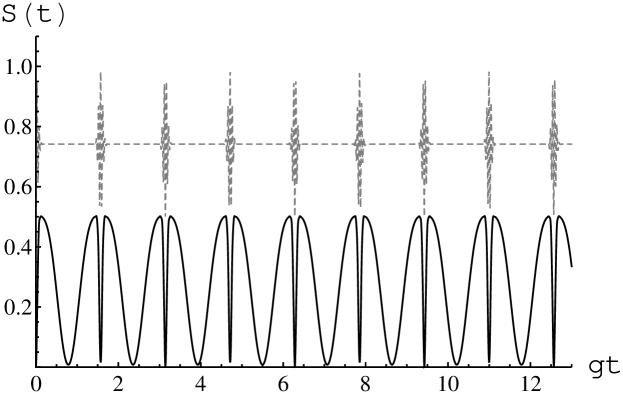
(b)

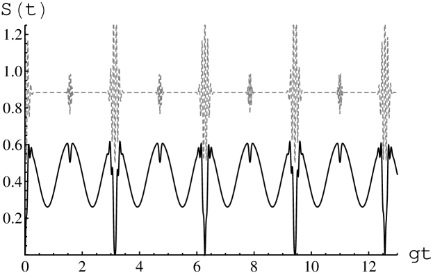
Figure 1: Time evolution of linear entropy for atomic initial states: (a) $\sqrt{1/2}(|+,-\rangle+|-,+\rangle)$ and (b) $|+,+\rangle$. The initial mean photon number $\overline{n}=30$ and phase of coherent state $\varphi=0$. Gray curves denote the possibility to find both atoms in excited stated $W_{++}+0.5$.

For the first model the dynamics of atomic linear entropy $S$ is presented in Fig. 1 for different initial atomic states and a coherent one-mode field of high intensity. We draw both values of linear entropy $S$ (black curves) and atomic possibilities to find both atoms in excited state (gray curves) in the figures. Fig. 1a demonstrates the time behavior of linear atomic entropy for the case when the atomic subsystem is prepared initially in state $A$ (or $B$). One can easily see from Fig.1a that there are two series of disentanglement times which exactly coincide with values predicted in Section II (see formulae (16) and (19)). The result confirms well the conclusions made on the basis of the analysis of the state vector asymptotic dynamics. As for the states $|+,+\rangle$ (or $|-,-\rangle,|+,-\rangle$ and $|-,+\rangle$) it can be clearly seen that the system evolves into entangled state and revive into its disentangled one only for times described exactly by formula (22)( see Fig. 1b).

So, one can see that all the results obtained by the linear entropy numerical calculations are in good accordance with the analytical expressions for wave function made in the previous section.

(a)

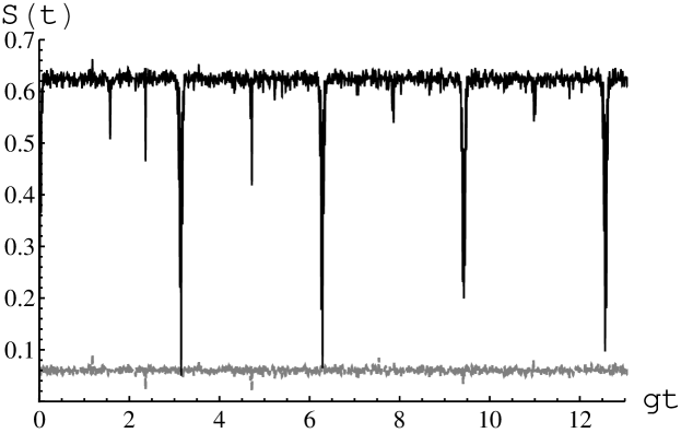
(b)

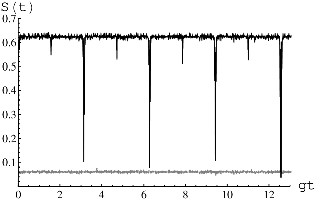
Figure 2: Time evolution of linear entropy for initial atomic state $(1/\sqrt{2})|+,-\rangle+|-,+\rangle$. The mean photon numbers $\overline{n}_{1}=\overline{n}_{2}=50$ (Fig 1a) and $\overline{n}_{1}=50,\overline{n}_{2}=150$ for (Fig 1b). The phases of the coherent states $\varphi_{1}=\varphi_{2}=0$. Gray curves denote the possibilities to find both atoms in exited states $|+,+\rangle$.

(a)

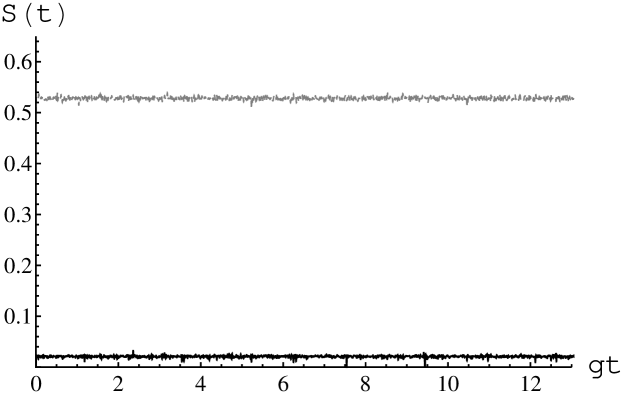
(b)

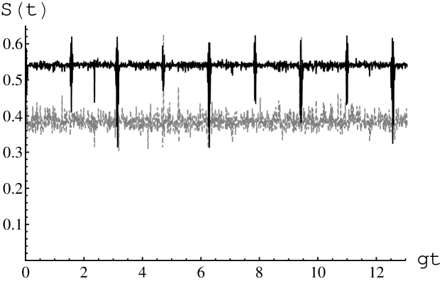
Figure 3: Time evolution of linear entropy for initial atomic states: $|\Phi_{3}\rangle$ (a) and $|+,+\rangle$ (b). The mean photon numbers $\overline{n}_{1}=\overline{n}_{2}=50$. Gray curves denote the possibilities to find both atoms in exited states $|+,+\rangle$.

For the second model the dynamics of atomic linear entropy is presented in Fig. 2 and 3 for different initial atomic states and a coherent two-mode field of high intensity. Fig 2 shows the time behavior of linear atomic entropy for initial atomic state $|\Psi_{A}\rangle$ and two choices of the mean photon numbers in two-mode coherent cavity field: $\bar{n}_{1}=\bar{n}_{2}=50$ (Fig. 2a) and $\bar{n_{1}}=50,\bar{n_{2}}=150$ (Fig. 2b). We draw both values of linear entropy $S$ (black curves) and atomic possibilities to find both atoms in excited state (gray curves) in the figures. One can easily see from Fig. 2 that there one series of disentanglement times which don’t depend on mean photon numbers and exactly coincide with values (23) predicted in Section 2 for states $A$ and $B$. We have obtained the atom-field entanglement which is periodically changed with completely full revival into pure disentangled state. Fig 2 shows the time behavior of linear atomic entropy for initial atomic state $|+,+\rangle$ and $\Phi_{3}$ for $\bar{n}_{1}=\bar{n}_{1}=50$. One can easily sea from Fig. 3a that for initial atomic state $|\Phi_{3}\rangle$ the system is really in a pure initial state disentangled state at any time. The analysis of analytical and numerical calculations of linear entropy for state $|+,+\rangle$ presented in Fig. 3b is too difficult. These problem will be solved in our following paper. So, one can see that all the results obtained by the linear entropy numerical calculations are in good accordance with the analytical expressions for wave function made in the previous section for states $A$ and $B$.

5 Conclusions

Two-atom one-mode and two-mode JCM with intensity-dependent coupling are considered in the paper. Atom-field entanglement is shown to occur in both models, the entanglement degree is estimated on the basis of analysis of wave-function behavior and a linear entropy criterion. The disentanglement is found to appear in the models for some initial atomic states and large coherent field inputs with different values of the mode intensities relation. We also estimate the periods of disentanglement for the models.

- (1) Jaynes, E.T., Cummings, F.W.: Comparison of quantum and semiclassical radiation theories with application to the beam maser. Proc. IEEE. 51, 89 (1963).
- (2) Yoo, H.Y., Eberly, J.H.: Dynamical theory of an atom with two and three levels interacting with quantized cavity fields. Phys. Reports. 118, 239 (1985).
- (3) Shore, B.W., Knight, P.L.: On the Jaynes-Cummings model. J.Mod.Opt. 40, 1195 (1993).
- (4) Walther, H., Varcoe, B.T.H., Englert, B.-G., Becker,T.: Cavity quantum electrodynamics. Rep.Prog. Phys. 69, 1325 (2006).
- (5) Haroche, S., Raimond, J.-M.: Exploring the Quantum. Atoms, Cavities, and Photons, Oxford University Press, New York, 2006.
- (6) Buluta, I, Ashhab, S, Nori, F.: Natural and artificial atoms for quantum computation. Rep. Prog. Phys. 74, 104401 (2011).
- (7) Barnett, S.M., Phoenix, S.J.D.: Entropy as a measure of quantum optical correlation. Phys. Rev. A40(5), 2404 (1989).
- (8) Phoenix, S.J.D., Knight, P.L.: Establishment of an entangled atom-field state in the Jaynes-Cumming model. Phys. Rev. A44(9), 6023 (1991).
- (9) Gea-Banacloche, J.: Collapse and revival of the state vector in the Jaynes-Cummings model: an example of state preparation by a quantum apparatus. Phys. Rev. Lett. 65, 3385 (1990).
- (10) Gea-Banacloche, J.: Atom- and field-state evolution in the Jaynes-Cummings model for large initial fields. Phys. Rev. A44, 5913 (1991).
- (11) Dung, H.T. Huyen, N.D.: State evolution in the two-photon atom-field interaction with large initial fields. Phys. Rev. A49, 473 (1994).
- (12) Nasreen, T., Zaheer, K.: Evolution of wave functions in the two-photon Jaynes-Cummings model: The generation of superpositions of coherent states. Phys. Rev. A49, 616 (1994).
- (13) Abdalla, M.S., Abdel-Aty, M., Obada A.-S.F.: Entropy and entanglement of time dependent two-mode Jaynes-Cummings model. Physica. A326, 203 (2003).
- (14) Larson, J., Garraway, B.M.: Dynamics of a Raman coupled model: Entanglement and quantum computation. J. Mod. Opt. 51, 1691 (2004).
- (15) Kudryavtsev, I.K., Lambrecht, A., Moya-Cessa, H., Knight, P.L.: Cooperativity and entanglement of atom-field states. J. Mod. Opt. 40, 1605 (1994).
- (16) Dung H.T., Huyen, N.D.: Two-atom-single mode radiation field interaction. State evolution, level occupation probabilities and emission spectra. J. Mod. Opt. 41, 453 (1994).
- (17) Song T.-Q., Feng, J., Wang W.-Z., Xu, J.-Z.: Effects of the relative coupling constants on the dynamic properties of a two-atom system. Phys.Rev. A51, 2648 (1995).
- (18) Bashkirov, E.K., Rusakova, M.S.: Atom-field entanglement in two-atom Jaynes-Cummings model with nondegenerate two-photon transitions. Opt. Comm. 281, 4380 (2008).
- (19) Bashkirov, E.K.: Entanglement in degenerate two-photon Tavis Cummings model. Phys. Scripta 82, 015401 (2010).
- (20) Bashkirov, E.K., Rusakova, M.S.: Entanglement for two-atom Tavis Cummings model with degenerate two-photon transitions in the presence of the Stark shift. Optik. 123, 1694 (2012).
- (21) Brune M., Raimond, J.M., Goy, P., Davidovich, L., Haroche, S.: Realization of a two-photon maser oscillator. Phys. Rev. Lett. 59, 1899 (1987).
- (22) Dell’Anno, F., De Siena, S., Illuminati, F.: Multiphoton quantum optics and quantum state engineering. Phys. Reports. 428, 53 (2006).
- (23) Bashkirov, E.K.: Dynamics of two-atom Jaynes- ummings model with nondegenerate two-photon transitions. Laser Phys. 16, 1218 (2006).
- (24) Singh, S., Ooi C.H.R., Amrita: Effects of cavity-field statistics on atomic entanglement in a two-mode Jaynes Cummings model with intensity-dependent coupling. J. Mod. Opt. 60, 666 (2013).
- (25) Napoli, A., Messina, A.: Dressed states and exact dynamics of intensity-dependent two-mode two-photon Jaynes-Cummings models. J. Mod. Opt. 43, 649 (1996).
- (26) Grinberg, H.: Beyond the rotating wave approximation. An intensity dependent nonlinear coupling model in two-level systems. Phys. Lett. A374 1481 (2010).
- (27) Singh, S., Amrita: Exact Solutions for Jaynes-Cummings Models with Non-degenerate Two-Photon Transitions in the Ladder Configuration. Int. J. Theor. Phys. 51, 838 (2012).
- (28) Singh, S., Ooi C.H.R., Amrita: Dynamics for two atoms interacting with intensity-dependent two-mode quantized cavity fields in the ladder configuration. Phys. Rev. A86, 023810 (2012).
- (29) Hekmatara, H., Tavassoly M.K.: Sub-Poissonian statistics, population inversion and entropy squeezing of two two-level atoms interacting with a single-mode binomial field: intensity-dependent coupling regime. Opt. Comm. 319, 121 (2014).