Chemical abundances of stars with brown-dwarf companions

Abstract

Context. It is well-known that stars with giant planets are on average more metal-rich than stars without giant planets, whereas stars with detected low-mass planets do not need to be metal-rich.

Aims. With the aim of studying the weak boundary that separates giant planets and brown dwarfs (BDs) and their formation mechanism, we analyze the spectra of a sample of stars with already confirmed BD companions both by radial velocity and astrometry.

Methods. We employ standard and automatic tools to perform an EW-based analysis and to derive chemical abundances from CORALIE spectra of stars with BD companions.

Results. We compare these abundances with those of stars without detected planets and with low-mass and giant-mass planets. We find that stars with BDs do not have metallicities and chemical abundances similar to those of giant-planet hosts but they resemble the composition of stars with low-mass planets. The distribution of mean abundances of $\alpha$-elements and iron peak elements of stars with BDs exhibit a peak at about solar abundance whereas for stars with low-mass and high-mass planets the [X_α/H] and [X_Fe/H] peak abundances remain at $\sim-0.1$ dex and $\sim+0.15$ dex, respectively. We display these element abundances for stars with low-mass and high-mass planets, and BDs versus the minimum mass, $m_{C}\sin i$, of the most-massive substellar companion in each system, and we find a maximum in $\alpha$-element as well as Fe-peak abundances at $m_{C}\sin i\sim 1.35\pm 0.20$ jupiter masses.

Conclusions. We discuss the implication of these results in the context of the formation scenario of BDs in comparison with that of giant planets.

1 Introduction

The most extended convention place the mass range of brown dwarfs (BDs) at $13-80\,M_{J}$ (being $M_{J}$ the mass of Jupiter), having enough mass to burn deuterium but not for hydrogen fusion (Burrows et al., 1997), i.e. in between the heaviest giant planets and the lightest stars. BDs above $\sim 65\,M_{J}$ are thought to fuse lithium and therefore the detection of the Li I $\lambda$ 6708 Å could be used to identify BDs, this is the so-called “Lithium Test” (Rebolo et al., 1992).

BDs were predicted by Kumar (1962) and Hayashi & Nakano (1963), but they were not empirically confirmed until 1995, when the first field brown dwarf was detected (Teide 1, Rebolo et al., 1995). This occurs the same year as the discovery of the first extra-solar planet (Mayor & Queloz, 1995). The first BD companion to a M-dwarf star was also discovered that year (GJ 229B, Nakajima et al., 1995). During the following two decades high-precision radial velocity (RV) surveys have shown that close BDs around solar-type stars are rare (Grether & Lineweaver, 2006, and references therein). Thus, at orbital separations of less than 10 AU, the frequency BD companions remains below 1 % (Marcy & Butler, 2000), whereas it is $\sim 7$ % for giant planets (Udry & Santos, 2007; Mayor et al., 2011) and $\sim 13$ % for stellar binaries (Halbwachs et al., 2003). The so-called ”Brown dwarf desert” may be interpreted as the gap between the largest-mass objects that can be formed in protoplanetary discs, and the smallest-mass clumps that can collapse and/or fragment in the vicinity of a protostar (Ma & Ge, 2014). The mass function, $dN/dm_{C}\propto m_{C}^{\alpha}$, of close planetary and stellar companions drops away ($\alpha\sim-1$) towards the BD mass range (Grether & Lineweaver, 2006). On the other hand, the mass function of isolated substellar objects is roughly flat or even with linear increase ($\alpha\sim 0$) down to $\sim 20$ $M_{J}$ (Chabrier, 2002; Kirkpatrick et al., 2012). This may point to a different formation scenario for close BD companions and BDs in the field and clusters.

Sahlmann et al. (2011) presented the discovery of nine BD companions from a sample of 33 solar-type stars that exhibit RV variations caused by a companion in the mass range $m_{C}\sin i\sim 13-80$ $M_{J}$. They used Hipparcos astrometric data (Perryman et al., 1997) to confidently discard some of the BD candidates. Including literature data, these authors quoted 23 remaining potential BD candidates. From CORALIE planet-search sample, they obtain an upper limit of 0.6% for the frequency of BD companions around Sun-like stars. Recently, Ma & Ge (2014) have collected all the BD candidates available in the literature including those in Sahlmann et al. (2011), some from the SDSS-III MARVELS survey (Ge et al., 2008) and some other RV surveys (e.g. Marcy & Butler, 2000).

The metallicity of stars with BD companions have been briefly discussed in (Sahlmann et al., 2011). They note that the sample is still too small to claim any possible metallicity distribution of stars hosting BDs. Ma & Ge (2014) extended the sample to roughly 65 stars with BD candidates, including dwarfs and giants, and stated that the mean metallicity of their sample is $\langle$[Fe/H]$\rangle$ $=-0.04$ ($\sigma=0.28$), i.e. remarkably lower than that of stars with giant planets ($\langle$[Fe/H]$\rangle$ $=+0.08$, Sousa et al., 2008, 2011). On the other hand, stars with only detected “small” planets (hereafter “small” planet refers to a low-mass planet, including Super-Earths and Neptune-like planets, with $m_{C}\sin i<30M_{\oplus}$, whereas “giant” planet refers to high-mass planets, including Saturn-like and Jupiter-like planets, with $30M_{\oplus}<m_{C}\sin i<13M_{J}$, see Section 3) do not seem to require high metal content to form planets within planetary discs (Sousa et al., 2008, 2011; Adibekyan et al., 2012c). Sousa et al. (2011) study a sample of 107 stars with planets (97 giant and 10 small planets) and found an average metallicity of stars with small planets at about $\langle$[Fe/H]$\rangle$ $=-0.11$, very similar to that of stars without detected planets (Sousa et al., 2008).

Currently, there are two well-established theories for giant planet formation: core-accretion scenario Pollack et al. (1996) and disc gravitational instability (Boss, 1997). The core-accretion model is more sensitive to the fraction of solids in a disc than is the disc-instability model. The formation of BDs has been also extensively studied. Two main mechanism have been proposed: molecular cloud fragmentation (Padoan & Nordlund, 2004), and disc fragmentation (Stamatellos & Whitworth, 2009). The latter mechanism, which requires a small fraction of Sun-like stars should host a massive extended disc, is able to explain most of the known BDs which may either remain bound to the primary star, or be ejected into the field (Stamatellos & Whitworth, 2009).

In this paper, we present a uniform spectroscopic analysis for a sample of stars with BD companions from Sahlmann et al. (2011) and we compare the results with those of a sample of stars with known giant and small planets from previous works (Adibekyan et al., 2012c). The aim of this work is to provide some information that could be useful to distinguish among the different and possible formation mechanisms of BD companions.

Table 1: Stellar parameters of the CORALIE sample

Star	$T_{\rm eff}$	$\log g$	$\xi_{t}$	$\rm[Fe/H]$	$M_{2}\sin i$	References
	$\rm[K]$	$\rm[dex]$	$\rm[cm/s]$	$\rm[dex]$	$[M_{J}]$
HD4747	$5316\pm 50$	$4.48\pm 0.10$	$0.79\pm 0.10$	$-0.21\pm 0.05$	$46.1$	2
HD52756	$5216\pm 65$	$4.47\pm 0.11$	$1.11\pm 0.13$	$0.13\pm 0.04$	59.3	1
HD74014	$5662\pm 55$	$4.39\pm 0.08$	$1.10\pm 0.07$	$0.26\pm 0.04$	49.0	1
HD89707	$6047\pm 42$	$4.52\pm 0.05$	$0.99\pm 0.06$	$-0.33\pm 0.03$	53.6	1
HD167665	$6224\pm 39$	$4.44\pm 0.04$	$1.18\pm 0.05$	$-0.05\pm 0.03$	50.6	1
HD189310	$5188\pm 50$	$4.49\pm 0.09$	$0.94\pm 0.10$	$-0.01\pm 0.03$	25.6	1
HD211847	$5715\pm 24$	$4.49\pm 0.05$	$1.05\pm 0.03$	$-0.08\pm 0.02$	19.2	1
HD3277a	$5539\pm 49$	$4.36\pm 0.06$	$0.91\pm 0.07$	$-0.06\pm 0.04$	64.7	1
HD17289a	$5924\pm 32$	$4.37\pm 0.04$	$1.15\pm 0.04$	$-0.11\pm 0.03$	48.9	1
HD30501a	$5223\pm 27$	$4.56\pm 0.08$	$1.18\pm 0.04$	$-0.06\pm 0.02$	62.3	1
HD43848a	$5334\pm 92$	$4.56\pm 0.15$	$1.35\pm 0.17$	$0.22\pm 0.06$	24.5	1
HD53680a	$5167\pm 94$	$5.37^{b}\pm 0.29$	$2.08\pm 0.31$	$-0.29\pm 0.04$	54.7	1
HD154697a	$5648\pm 45$	$4.42\pm 0.05$	$1.04\pm 0.06$	$0.13\pm 0.04$	71.1	1
HD164427Aa	$6003\pm 27$	$4.35\pm 0.03$	$1.19\pm 0.03$	$0.19\pm 0.02$	48.0	1
HIP103019a	$4913\pm 115$	$4.45\pm 0.28$	$0.54^{c}\pm 0.10$	$-0.30\pm 0.06$	52.5	1
HD74842d	$5517\pm 38$	$4.50\pm 0.06$	$1.01\pm 0.06$	$-0.08\pm 0.03$	–	3
HD94340d	$5902\pm 26$	$4.19\pm 0.03$	$1.30\pm 0.03$	$0.11\pm 0.02$	–	3
HD112863d	$5342\pm 36$	$4.57\pm 0.07$	$1.08\pm 0.07$	$-0.11\pm 0.03$	–	3
HD206505d	$5392\pm 44$	$4.46\pm 0.07$	$1.02\pm 0.07$	$0.11\pm 0.03$	–	3

(1) Sahlmann et al. (2011); (2) Santos et al. (2005); (3) This work.

2 Observations

We analyse data for two different samples obtained with two different telescopes and instruments: stars with BDs with spectroscopic data at resolving power $R\sim 50,0000$ taken at the 1.2m-Euler Swiss Telescope equipped with the CORALIE spectrograph (Udry et al., 2000) and stars with planetary companions observed with the HARPS spectrograph (Mayor et al., 2003) with $R\sim 115,000$ installed at the 3.6m-ESO telescope, both of them at La Silla Observatory (ESO) in Chile.

The individual spectral of each star were reduced in a standard manner, and latter normalized within the package IRAF, using low-order polynomial fits to the observed scontinuum.

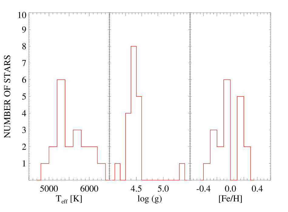
Figure 1: Histograms of the stellar parameters $T_{\rm eff}$, $\log{g}$ and $\rm[Fe/H]$ of our CORALIE sample.

3 Sample description and stellar parameters

3.1 Stars with BD-companion candidates

Our stellar sample has been extracted mostly from F-, G- and K-type main-sequence stars of the CORALIE RV survey (Udry et al., 2000). This sample consists of 15 stars with BD companion candidates reported in Sahlmann et al. (2011), for which the minimum mass, $m_{C}\sin i$, of most massive companion is in the brown-dwarf mass range ($13-80\,M_{J}$). One of these 15 stars, HIP 103019, has been extrated from the HARPS RV survey (Mayor et al., 2003). In Table 1 we provide the minimum mass of these 15 BD candidates. Sahlmann et al. (2011) were also able to derive the orbital inclination, $i$, by using astrometric measurements from Hipparcos (Perryman et al., 1997; van Leeuwen, 2007). This allowed them to confidently exclude as BD candidates eight stars from the initial sample of 15 stars because the current mass determinations, $m_{C}$, place them in M-dwarf stellar regime. Stellar parameters of the sample of 14 stars were collected from Sahlmann et al. (2011) and one star from Santos et al. (2005). Four additional stars from the CORALIE sample without detected BD companions were analyzed as a comparison/control sample (see Table 1). In Fig.1 we show the histograms of $T_{\rm eff}$, $\log g$, and [Fe/H] for our stellar sample. We only display those stars with available $m_{C}\sin i$ values in Table 1.

We note that Ma & Ge (2014) also collected a sample 65 stars with BD candidates: 43 stars, 27 dwarfs and 15 giants, with $m_{C}\sin i$ values in the range 13-90 $M_{J}$. Two stars, included in Ma & Ge (2014) as BD candidates, HD 30501 and HD 43848, were discarded by Sahlmann et al. (2011), probably because they have $m_{C}$ values above but close to the 80 $M_{J}$ boundary. Fig.3 depicts the minimum mass of the BD companion $m_{c}\sin i$ and orbital period against metallicity [Fe/H], including stars of our sample as well as those stars in the sample of Ma & Ge (2014) for comparison. We separate giant ($\log g<4$) and dwarfs ($\log g>4$) stars. The stars with BD candidates spread over a wide range of orbital periods, a minimum masses of the BDs, and stellar metallicities.

3.2 Stars with planetary-mass companions

The HARPS sub-sample (HARPS-1 sample in Adibekyan et al., 2012c) used in this work contains 451 stars (Sousa et al., 2008; Neves et al., 2009), both with and without planetary companions. We collect the minimum mass of the most-massive planet in each planetary system from the encyclopaedia of extra-solar planets . The planetary-mass sample is separated in two groups: (i) small planets (SP; super-Earth like and Neptune like planets) with masses of $m_{C}\sin i<\sim 0.094$ $M_{J}$ ($\sim 30M_{\oplus}$), and (ii) giant planets (GP; Saturn like and Jupiter like planets) with masses in the range $0.094<m_{C}\sin i\;[M_{J}]<13$. Two of the stars with giant planets, HD 162020 and HD 202206, within the HARPS sample have companion masses above 13 $M_{J}$ and will be considered as BDs hereafter.

Therefore, our final sample of confirmed BDs contains 9 dwarf stars, with companions in the mass range $m_{C}\sin i\sim 13-80$ $M_{J}$. In the following, we may refer to “BD-host stars” to stars with confirmed BDs, i.e. with $m_{C}\sim 13-80$ $M_{J}$, and “stars with discarded BDs” to those with $m_{C}\sin i\sim 13-80$ $M_{J}$ but $m_{C}>80$ $M_{J}$, according to Sahlmann et al. (2011). The sample of planet-host stars contains 25 stars with small planets and 78 stars with giant planets. In Table 9 we provide the minimum mass of the most-massive planet in each planetary system of the stars in the HARPS sample.

4 Automatic codes for EW measurements: ARES versus TAME.

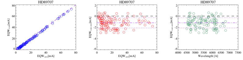
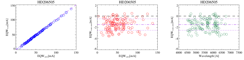
Figure 2: ARES versus TAME graphics for the stars HD 89707 ($\mathrm{S/N}\sim 110$) and HD 206505($\mathrm{S/N}\sim 70$). Left panels: EW measured with TAME versus ARES. The 1:1 correspondence is shown as a dashed line. EW differences, $\rm EW_{TAME}-EW_{ARES}$, versus $\rm EW_{ARES}$ (middle panels) and spectral line wavelength (right panels). Dash-dotted lines define the mean value of the data points, and dotted lines define the mean plus the standard deviation.

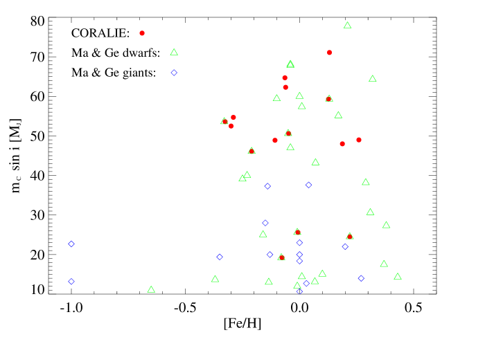
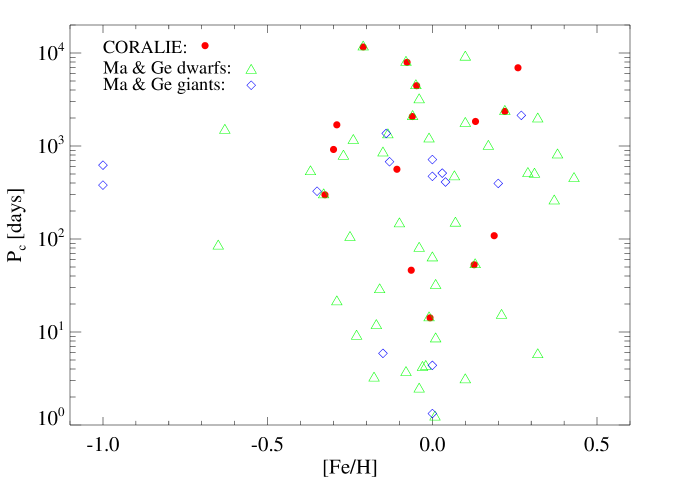
Figure 3: Minimum mass of the most-massive companion, $m_{C}\sin i$, and orbital period, $P_{C}$, versus the metallicity of stars with BDs. The CORALIE sample is depicted as filled symbols, and the sample in Ma & Ge (2014) is displayed as empty symbols, separated among giant and dwarf stars.

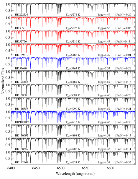
Figure 4: High-resolution normalized spectra of late G-, K-type stars: CORALIE spectra of coolest stars in the sample (black), HARPS spectra (red) of cool stars from the HARPS database (e.g. Sousa et al., 2008) and the CORALIE spectrum (blue) of HD 53680 and the HARPS spectrum (blue) of HIP 103019. The spectra are depicted following a sequence with decreasing $T_{\rm eff}$ from top to bottom.

We measure the equivalent widths (EWs) of spectral lines using the linelists in Sousa et al. (2008); Neves et al. (2009); Adibekyan et al. (2012c) using automatic tools. We explore two different automatic codes for EWs spectra analysis: the automatic C++ based code ARES (Sousa et al., 2007) and a new IDL based code named TAME (Kang & Lee, 2012). In order to compare these two automatic codes, we measure the EWs of CORALIE sample with the same input parameters to these two codes.

In Fig. 2, we compare the EWs measured using TAME, $EW_{\rm TAME}$, against those estimated using ARES, $EW_{\rm ARES}$. The mean value of the EW differences $EW_{\rm TAME}-EW_{\rm ARES}$ is found at $\sim-1.2\,m\AA$ and $\sim-1.5\,m\AA$ for the stars HD 89707 star ($\mathrm{S/N}\sim 110$) and HD 206505($\mathrm{S/N}\sim 70$). The TAME code is very slightly underestimating the EW compared to ARES measurements, and the scatter of these comparisons is lower than $\sim 1.5\,\rm m\AA$. These EW differences do not exhibit any remarkable dependence on wavelength. We also tested whether the signal-to-noise ratio (S/N) from our stellar spectra is the source of this observed tendency and no trend has been found. The mean value of the EW differences is fluctuating in the $-2\,\rm m\AA$ to $-1\,\rm m\AA$ range. The standard deviation of the EW differences improves slightly as the S/N increases, but it oscillates between $0.5\,\rm m\AA$ to $1.5\,\rm m\AA$.

This analysis lead us to conclude that both programs show a good agreement and their differences are not significant and do not have any relevant impact on the chemical abundance analysis, within the typical error bars of the EW-based chemical abundance analysis.

Table 2: Fe i and Fe ii abundances and standard deviations

Star	$\rm[FeI/H]$	$\rm[FeII/H]$
HD4747	$-0.28\pm 0.06$	$-0.28\pm 0.10$
HD52756	$0.09\pm 0.10$	$0.03\pm 0.15$
HD74014	$0.23\pm 0.07$	$0.16\pm 0.11$
HD89707	$-0.35\pm 0.09$	$-0.40\pm 0.12$
HD167665	$-0.11\pm 0.10$	$-0.09\pm 0.10$
HD189310	$-0.03\pm 0.10$	$-0.10\pm 0.22$
HD211847	$-0.10\pm 0.06$	$-0.11\pm 0.09$
HD3277	$-0.10\pm 0.05$	$-0.12\pm 0.08$
HD17289	$-0.13\pm 0.08$	$-0.09\pm 0.13$
HD30501	$-0.09\pm 0.10$	$-0.14\pm 0.18$
HD43848	$0.18\pm 0.13$	$0.14\pm 0.25$
HD53680⋆	$-0.37\pm 0.24$	$-0.61\pm 0.41$
HD154697	$0.10\pm 0.06$	$0.06\pm 0.10$
HD164427A	$0.15\pm 0.06$	$0.14\pm 0.09$
HIP103019⋆	$-0.34\pm 0.29$	$-0.68\pm 0.45$
HD74842	$-0.12\pm 0.09$	$-0.10\pm 0.11$
HD94340	$0.10\pm 0.06$	$0.08\pm 0.11$
HD112863	$-0.12\pm 0.09$	$-0.14\pm 0.10$
HD206505	$0.10\pm 0.09$	$0.08\pm 0.12$

5 Chemical abundances

We compute the EWs using ARES for consistency with chemical abundance analysis in Adibekyan et al. (2012c). We also use version 2010 of the MOOG  code (Sneden, 1973) together with Kurucz ATLAS9 stellar model atmospheres (Kurucz, 1993) for chemical abundance determination.

We first check the Fe i and Fe ii abundances, using the line list from Sousa et al. (2008). The high dispersion, $\sigma$, of the Fe abundances (see Table 2) of the stars HD 53680 and HIP 103019 suggests that these stars may have lower effective temperatures than those given Table 1. In Fig. 4 we depict the normalized spectra of the coolest stars in the sample together with some spectra of late-G, K-type dwarfs from the HARPS database (e.g. Sousa et al., 2008). The $H\alpha$ profiles of these two stars do not follow the sequence of temperatures but they appear to be the coolest objects in Fig. 4. In addition, these stars were discarded as candidates of BDs by Sahlmann et al. (2011). We note the unusually high surface gravity estimated for the star HD 53680 which is likely spurious, consistent with the large scatter in the Fe abundances and the difference between Fe i and Fe ii abundances. This star is catalogued in the SIMBAD database as a K6V star in a visual binary system. The narrow $H\alpha$ line and the large dispersion in Fe i and Fe ii abundances may indicate an even later spectral type. For these reasons, they may deserve further analysis and from this point on, we will not consider them.

We use the linelist in Neves et al. (2009) on 17 stars of CORALIE remaining sample (seven stars with confirmed BDs, six with discarded BD candidates, and four without detected BD companions) to derive element abundances of Na i, Mg i, Al i, Si i, Ca i, Sc i, Sc ii, Ti i, Ti ii, V i, Cr i, Cr ii, Mn i, Co i and Ni i. Some lines of the original list are not considered: lines non-detected by ARES, lines discarded in the Adibekyan et al. (2012c), and lines whose abundances were out of the $3\sigma$ range. The abundance results are shown in Tables 5, 6 and 7. The chemical abundances of the HARPS sample were obtained from Adibekyan et al. (2012c) where they use exactly the same tools and model atmospheres.

6 Discussion

Gonzalez (1997); Gonzalez & Laws (2000) already noticed that giant planet hosts tend to be more metal-rich than stars without detected planets. Santos et al. (2001) provided supporting evidences of a metal-rich origin of giant-planet host stars and following studies confirmed this result (e.g. Santos et al. 2004, 2005; Valenti & Fischer 2005). Recent studies show that Neptune and super-Earth class planet hosts have a different metallicity distribution, more similar to stars without planets (e.g. Udry et al., 2006; Sousa et al., 2008, 2011; Ghezzi et al., 2010; Mayor et al., 2011; Buchhave et al., 2012).

In this section, we inspect the abundance ratios of different elements, $\rm[X/Fe]$, as a function of the metallicity for our BD-companion stellar sample, as well as comparing them with the planetary-companion stars analized by Adibekyan et al. (2012c). We also study the distributions of different element abundances in different samples and we compare them with other stars with and without planets as a function of the minimum mass of the most-massive companion of each host star, $m_{C}\sin{i}$.

6.1 Galactic abundance trends

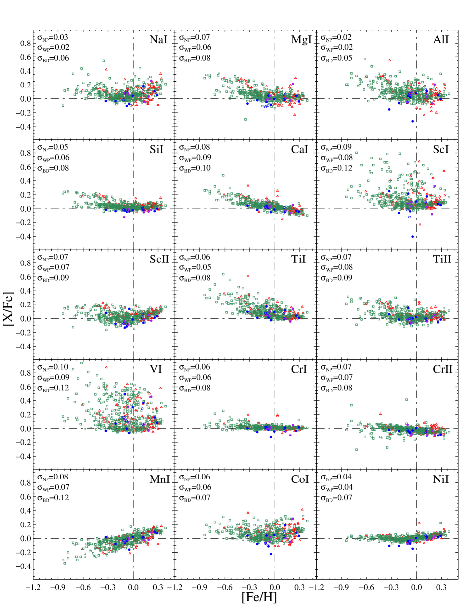
Figure 9: Element abundance ratios $[{\rm X/Fe}]$ against [Fe/H] for the samples of stars without planets (green empty squares), stars with planets (red empty triangles), BD-host stars (blue filled circles), stars without known BD companions from the CORALIE sample (blue empty circles), and stars with discarded BD candidates (violet filled circles). At the top-left corner of each panel, the mean standard deviation of the abundance measurements are shown for the stars without planetary companion ($\sigma_{\rm NP}$), stars with planets ($\sigma_{\rm WP}$) and stars with confirmed BD companions ($\sigma_{\rm BD}$) respectively.

The abundances of the refractory elements in CORALIE sub-sample exhibit the similar behaviour as other stars with and without planets analysed in previous works (Neves et al., 2009; Adibekyan et al., 2012c) (see Fig. 9).

Stars with BDs follow the galactic abundance trend except for some particular elements (Co, Si, Sc) where the abundances are slightly lower than expected. These exceptions may be due to the small number of lines to achieve a reliable mean abundance in certain elements (e.g. ScI for HD 167665). Stars with BD companions appear to be located at an intermediate range of metallicity, between stars with and without planets.

In Fig. 5 we display the mean abundance ratio of the $\alpha$-elements Mg, Si, Ca and Ti (with [X_α/H] computed as the sum of individual element abundances [X/H] divided by 4, and [X_α/Fe]=[X_α/H]-[Fe/H]) against the metallicity of stars with small and giant planets from (Adibekyan et al., 2012b) together with stars with BDs. The range of metallicities of stars with confirmed BDs seems to be narrower than that of the planet hosts although this may be not statistically significant due to the small number of stars in the BD sample. Adibekyan et al. (2012b, a) remarked that stars with both small and giant planets at low metallicities [Fe/H] $<-0.3$ dex, tend to be $\alpha$-enhanced and therefore to belong chemically to thick-disk population. There is only one star with BD at these relatively low metallicities, at [Fe/H] $\sim-0.35$ dex, showing a relatively low [X_α/Fe] ratio, and therefore the question whether this behaviour still holds for BD hosts remains open. The $\alpha$-element abundance ratios $[{\rm X_{\alpha}/Fe}]$ of BD hosts seem to be consistent with the Galactic trend at higher metallicities, although there are some stars at metallicities below solar with relatively low [X_α/Fe] ratios, even below the trend described by the stars without detected planets of the HARPS sample. Stars with discarded BDs and without detected BD candidates also follow the general abundance trend.

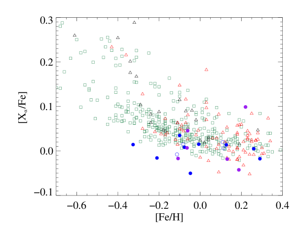
Figure 5: $\alpha$-element abundance ratios $[{\rm X_{\alpha}/Fe}]$ against [Fe/H] for the samples of stars without planets (green empty squares), with small planets (black empty triangles), with giant planets (red empty triangles), BD-host stars (blue filled circles), stars without known BD companions from the CORALIE sample (blue empty circles), and stars with discarded BD candidates (violet filled circles).

6.2 Element abundance distributions

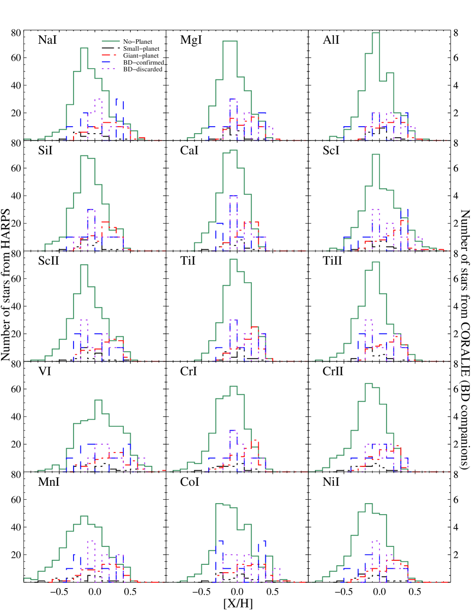
Figure 10: Histogram of element abundances, $[{\rm X/H}]$, of the samples of stars without planets (green continuum line), stars with low-mass planets (black dashed-double-dotted line), stars with giant planets (red dashed-dotted line), stars with confirmed BD companions (blue dashed line) and stars with discarded BD candidates (violet dotted line). The left y-axis of the top panel is labeled with the number of stars with and without small and giant planets whereas the right y-axis shows the number of stars with BD-companion candidates.

The histograms displayed in Fig. 10 allow us to study the abundance distribution [X/H] of our sample for each element. Stars without planets have a maximum abundance at $\sim-0.1$ for most speciess. Stars with giant planets exhibit a more metal-rich maximum at $\sim 0.2-0.3$ dex, while the stars with small planets (whose maximum is at $\sim-0.1$ dex) resemble to the “single” ones. This general behaviour already noticed in previous papers (Neves et al., 2009; Adibekyan et al., 2012b), is in a good agreement with the so-called metallicity effect, i.e. the strong correlation between stellar metallicity, and the likelihood of finding giant planets (Santos et al., 2001).

The abundance distribution of the sample of confirmed BD-host stars appears to be located in between the stars with small planets and stars with giant planets. In fact, some element distributions (Na, Si, Mg, Mn) are more similar to those of giant planets, whereas for others elements (Ti, Cr, Co, Ni) the behaviour is closer to the stars without planets (see Fig. 10).

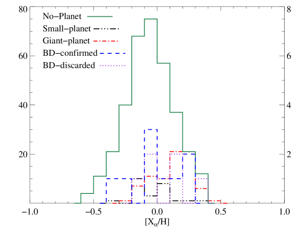
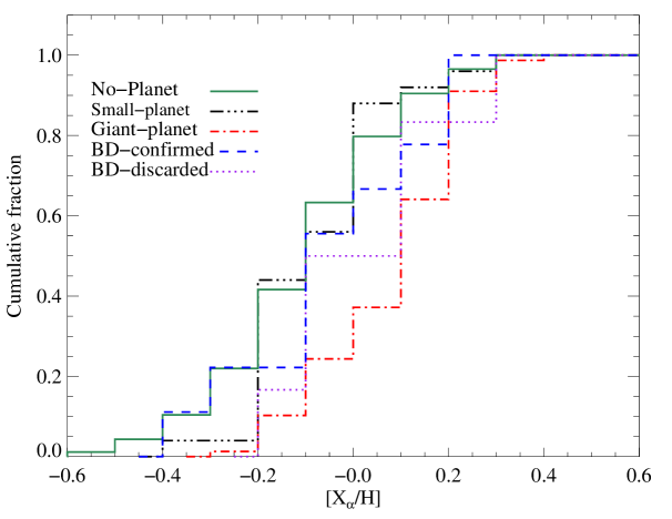
Figure 6: Histogram of $\alpha$-element abundances, $[{\rm X_{\alpha}/H}]$, (top panel) of the samples of stars without planets (green continuum line), stars with small planets (black dashed-double-dotted line), stars with giant planets (red dashed-dotted line), stars with confirmed BD companions (blue dashed line) and stars with discarded BD candidates, i.e. binaries with low-mass M-dwarf companions (violet dotted line). The left y-axis of the top panel is labeled with the number of stars with and without small and giant planets whereas the right y-axis shows the number of stars with BD-companion candidates. The lower panel shows cumulative histogram.

In Figs. 6 and 7 we display the distribution and cumulative histograms of the $\alpha$-element abundances (including the species Mg i, Si i, Ca i, Ti i), $[{\rm X_{\alpha}/H}]$, and the Fe-peak element abundances (including the species Cr i, Mn i, Co i, Ni i), $[{\rm X_{\rm Fe}/H}]$. Here it appears more clear the fact that confirmed BDs seems to behave differently from giant planets. Although the sample is small, it may tentatively point to a bimodal distribution with two peaks, one at the position of the small planet distribution and one at the position of the giant planets. However, the mean values of the $[{\rm X_{\alpha}/H}]$ and $[{\rm X_{\rm Fe}/H}]$ abundances are roughly solar. The $[{\rm X_{\alpha}/H}]$ and $[{\rm X_{\rm Fe}/H}]$ cumulative histograms support the previous statement. Stars with small planets and without detected planets go together, whereas the stars with BDs exhibit a slightly different behaviour with a later growth of the cumulative histogram which resembles that of stars with small planets only at [X/H] $>0.1$ dex. The cumulative histogram of stars with giant planets clearly manifest a later increase towards high metallicities reaching the saturation at [X/H] $\sim 0.3$ dex. We perform a K-S test to statistically evaluate the significance of this apparerent different behaviour (see Table 3). This test provides a clear difference between the BD-host sample and the GP sample but the SP and NP sample seems to be statistically very similar to the BD sample. The number of stars with confirmed BDs must be increased in order to be able to distinguish these populations. On the other hand, in Table 3 we also show the same K-S test for the stars with discarded BDs which are in fact binaries hosting low-mass M dwarfs. Although again there are only six stars in this sample, it appears to be statiscally different from all the samples of GP, SP and NP, especially for the Fe-peak element abundances. However, the significance is lower than the comparison with confirmed BD-host stars.

Table 3: Significance of the K-S test of the BD sample

BD⋆	SP	GP	NP
	$\alpha$-element abundances
Discarded	0.33	0.42	0.31
Confirmed	0.87	0.08	0.83
	Fe-peak element abundances
Discarded	0.15	0.53	0.19
Confirmed	0.72	0.13	0.77

6.3 Abundance ratios $\rm[X/H]$ against companion mass

The $m_{C}\sin i$ values of the BD candidates in our sample are higher than $13\,M_{J}$ (the star with the lightest BD companion analyzed in this work is orbiting HD 211847, $m_{C}\sin i\sim 19.2\,M_{J}$) but two of the most-massive giant planets of HARPS sample exceed this value. The boundary between brown dwarfs and giant planets has been extensively investigated in the literature, and some works agree with the definition that brown dwarfs can burn the deuterium that is present when they form, and giant planets cannot (e.g. Burrows et al., 1997). In Bodenheimer et al. (2013), the borderline between giant planets and brown dwarfs is found to depend only slightly on different parameters, such as core mass, stellar mass, formation location, solid surface density in the protoplanetary disc, disc viscosity, and dust opacity. More than 50 % of the initial deuterium is burned for masses above $11.6-13.6$ $M_{J}$, in agreement with previous determinations that do not take the formation process into account. Thus, we keep the mass $\sim 13M_{J}$ to distinguish among giant planets and brown dwarfs.

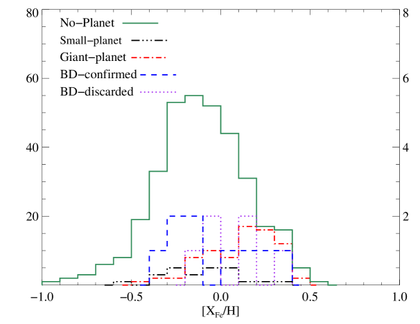
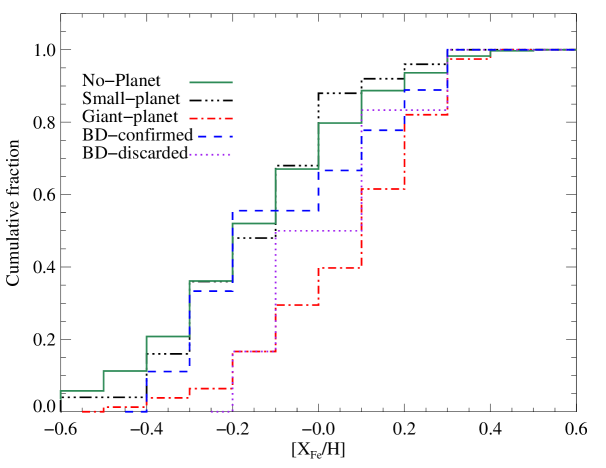
Figure 7: Same as Fig. 6 but for Fe-peak element abundances.

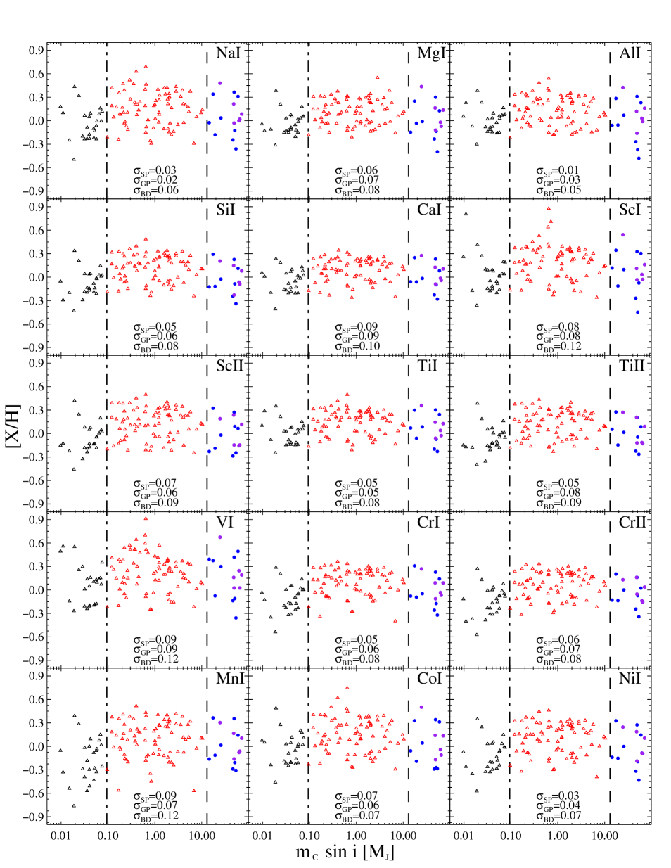
Figure 11: Element abundances, $\rm[X/H]$, against the minimum mass of the most-massive companion, $m_{C}\sin i$. Black empty triangles refer to stars with small planets, red empty triangles to stars with giant planets, and blue filled circles to stars with confirmed BDs, and violet filled circles to stars with discarded BD candidates. At the bottom of each panel, standard deviations of the mean element abundances are shown for stars without planets ($\sigma_{\rm NP}$), stars with planets ($\sigma_{\rm WP}$) and stars with confirmed BD companions ($\sigma_{\rm BD}$), respectively.

The metal-content of stars at birth surely affects the formation of the planetary-mass companions, but is this also true for stars with BD companions? To answer this question we depicted in Fig 11 the chemical element abundances, [X/H], as a function of the minimum mass of the most-massive substellar companion, that could be a small planet, a giant planet or a brown dwarf according to their $m_{C}\sin i$ values. Qualitatively, these element abundances seem to progressively increase with the companion mass from small planets until reaching a maximum at about 1 $M_{J}$ and then slightly decrease when entering in the BD regime. The scatter in [X/H] may be due to the different intrinsic metallicities of the stars at every bin in $m_{C}\sin i$.

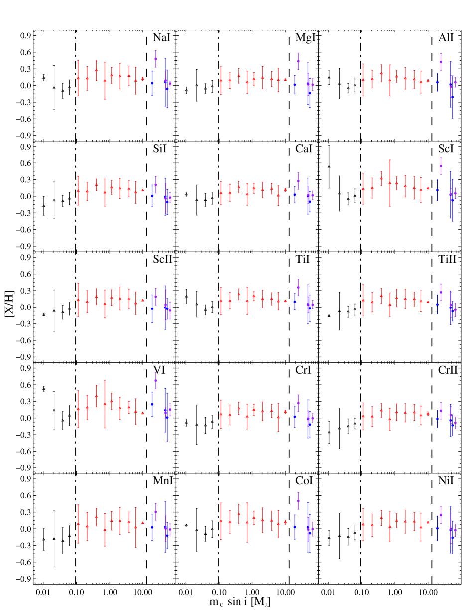
Figure 12: Mean element abundances versus the minimum mass of the most-massive companion, $m_{C}\sin i$, computed in equal-size bins appropriated for the logarithmic scale of companion masses. Error bars represent the standard deviation of the mean.

In Fig. 12 we display the mean values of these element abundances, [X/H], in bins of $m_{C}\sin i$. The standard deviations from the mean values are different for every element, but they stay around $0.15-0.2$ dex. These mean element abundances keep roughly constant for small planets with masses lower than $0.04\,M_{J}$. From this point on, the abundances grow with the companion mass even in the giant-planet companion range, from low-mass up to Jupiter-mass planets, reaching a maximum in $\sim 0.8\,M_{J}$ (see e.g. Si i, Ti i, Cr i, and Ni i). For more massive giant-planet companions, these abundances start to decrease slowly with the companion mass towards high-mass BD companions. The stars with BD-companion just follow the decreasing trend of the stars with giant planets.

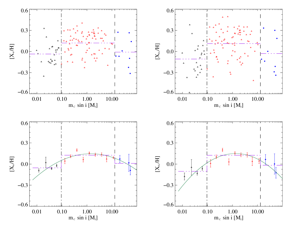
Figure 8: Abundance ratios $[{\rm X_{\alpha}/H}]$ and $[{\rm X_{Fe}/H}]$ against minimum mass of the most-massive companion $m_{C}\sin i$ of $\alpha$-elements (left-top panel) and iron-peak elements (right-top panel), for stars with small planets (black empty triangles), with giant planets (red empty triangles), with confirmed BD companions (blue filled circles). The average values are shown as violet three-dotted-dashed lines. Lower panels show the mean abundances of stars with small and giant planets, and confirmed BD companions, in equal-sized bins appropriated for the logarithmic scale of companion masses as in Fig. 12. Error bars represents the standard deviation of the mean divided by the square root of the number of stars in each bin. The green solid line depicts the parabolic fit of the data, whereas the violet three-dotted-dashed lines show the zero-order fits.

We decided to also use the mean values of the $\alpha$-elements, $[{\rm X_{\alpha}/H}]$ and Fe-peak elements, $[{\rm X_{\rm Fe}/H}]$, of each star in these samples. Thus, in Fig. 8 we display these abundances as a function of the minimum mass of the most-massive companion, $m_{C}\sin i$. The scatter of these abundances is high due to the different global metallicity of different stars. The average values of these abundances are shown in Table 4 for the SP, GP and BD samples. One can see in Fig. 8 the different levels of these three samples, although the BD sample shows an average value consistent with the SP sample within the error bars (see Table 4).

Table 4: Mean abundance of SP, GP and BD samples

Method⋆	SP	GP	BD
	$\alpha$-element abundances
Average	$-0.04\pm 0.03$	$0.12\pm 0.02$	$-0.01\pm 0.07$
Fit	$-0.05\pm 0.01$	$0.12\pm 0.01$	$0.01\pm 0.04$
	Fe-peak element abundances
Average	$-0.11\pm 0.04$	$0.11\pm 0.02$	$-0.03\pm 0.08$
Fit	$-0.10\pm 0.02$	$0.12\pm 0.01$	$-0.02\pm 0.05$

In the lower panels of Fig. 8, we depict the weighted average of these abundances at each mass bin and there the trend appears more clear. We fit a parabolic function, using the IDL routine curvefit, to these mean values of the $\alpha$-element and Fe-peak element abundances. The peaks of these trends have a maximum of abundance at $\sim 0.15\pm 0.01$ dex and companion mass of $m_{C}\sin i\sim 1.42\pm 0.17$ and $1.32\pm 0.18$ $M_{J}$, respectively. The parabolic fit, with $\chi_{\nu}^{2}$ values of 3.2 and 2.3 respectively, provides a better representation of the average abundances than the linear fit (with $\chi_{\nu}^{2}\sim 10.5$ and 8.6). We perform an F-test to confirm that the parabolic curve fits these data set better than the linear fit. We use the IDL routine mpftest from Markwardt library. The result reveals a significance level of $1\times 10^{-5}$ for $\alpha$-elements ($\rm F=45.8$) and $3\times 10^{-6}$ for iron-peak elements ($\rm F=37.9$), implying that the parabolic fit is significantly better than the linear.

We also perform a fit of a three zero-order function of three levels describing the SP, GP and BD samples and the values are given in Table 4, with $\chi_{\nu}^{2}$ values of 3.0 and 2.6 for $\alpha$-element and Fe-peak element abundances, respectively. We compare this 3-step model with the parabolic fit using an F-test, resulting in $F$ values of -0.5 and 0.6 which gives a significance level of 0 and $0.5$ for $\alpha$-elements and Fe-peak elements, respectively. Therefore, the 3-step model provides a similar description of the data than the parabolic fit. We also check that a 2-step model provides a worse fit than the 3-step model (with $\chi_{\nu}^{2}\sim 3.6$ and 3.1 for $\alpha$-elements and Fe-peak elements, respectively).

Finally, Sahlmann et al. (2011) noticed that there is a lack of BD companions with masses in the range $m_{C}\sin i\sim$ 35–55 $M_{J}$. More recently, Ma & Ge (2014) have collected the known BD companions from different studies and confirm this gap for stars with for periods shorter than 100 days. Although the statistics may be still poor these authors suggest that BD companions below this gap, i.e. with $m_{C}\sin i<42$ $M_{J}$, may have formed in protoplanetary disks as giant planets, probably through the disk instability-fragmentation mechanism (Boss, 1997; Stamatellos & Whitworth, 2009), whereas BD companions with $m_{C}\sin i>42$ $M_{J}$ may have formed by molecular cloud fragmentation as stars (Padoan & Nordlund, 2004; Hennebelle & Chabrier, 2008).

In bottom panels of Fig. 8 we may see that on average stars with BDs at masses $m_{C}\sin i$ below 42 $M_{J}$ have higher $\alpha$-element and Fe-peak element abundances than stars above this mass. In fact, stars with massive BD companions have more similar abundances to those of stars without planets. This might tentatively support the above statement with the low-mass BD companions being formed in protoplanetary disks as giant planets, and the high-mass BDs being formed by cloud fragmentation as stars.

7 Conclusions

We have analyzed a subsample of stars with candidate BD companions from the CORALIE radial velocity survey. We derive chemical abundances of several elements including $\alpha$-elements and Fe-peak elements. A comparison with the chemical abundances of stars with giant planets shows that BD-host stars seem to behave differently. In particular, we compute the abundance histograms [X_α/H] and [X_Fe/H], revealing a mean abundance at about solar for the BD-host sample whereas for stars without planets (NP) and with small planets (SP) remains at $-0.1$ dex, and for stars with giant planets (GP) at roughly$+0.10$ dex. The cumulative histograms of [X_α/H] and [X_Fe/H] abundances exhibit the same situation, with the stars without planets and with small planets going together, similarly to the stars with BDs. However, the stars with giant planets reach a later saturation at [X/H] $\sim 0.3$ dex. A Kosmogorov-Smirnov (K-S) test does not show a statisticallly significant difference between the cumulative distribution of SP, NP and BD samples, but clearly separates the GP and BD samples.

Finally, we depict the [X_α/H] and [X_Fe/H] abundances versus the minimum mass of the most-massive substellar companion, $m_{C}\sin i$, and we find a peak of these element abundances for a companion mass $m_{C}\sin i\sim 1.3-1.4\,M_{J}$, with the abundances growing with the companion mass from small planets to Jupiter-like planets and after decresing towards massive BD companions. A 3-step model also provides a similar description of the data with no statistically significant difference with the parabolic model. Recently, Sahlmann et al. (2011) and Ma & Ge (2014) have suggested that the formation mechanism may be different for BD companion below and above 42 $M_{J}$. We find that BDs below this mass tend to have higher abundances than those above this mass, which may support this conclusion and BDs with $m_{C}\sin i<42$ $M_{J}$ may form by disk instability-fragmentation whereas high-mass BD may form as stars by cloud fragmentation.

8 Acknowledgments

D.M.S. is grateful to the Spanish Ministry of Education, Culture and Sport for the financial support from a collaboration grant, and to the PhD contract funded by Fundación La Caixa. J.I.G.H. and G.I. acknowledge financial support from the Spanish Ministry project MINECO AYA2011-29060, and J.I.G.H. also from the Spanish Ministry of Economy and Competitiveness (MINECO) under the 2011 Severo Ochoa Program MINECO SEV-2011-0187. N.C.S. acknowledges the support by the European Research Council/European Community under the FP7 through Starting Grant agreement number 239953, and the support in the form of a Investigador FCT contract funded by Fundação para a Ciência e a Tecnologia (FCT) /MCTES (Portugal) and POPH/FSE (EC). This research has made use of the IRAF facilities, and the SIMBAD database, operated at the CDS, Strasbourg, France.

Appendix A Tables of chemical abundaces

In this appendix we provide all the tables containing the element abundances of the 17 stars within the CORALIE sample, the first 13 stars with BD-companion candidates (for more details see the text of Section 3, 7 confirmed BDs and 6 discarded BDs, and four stars as comparison sample.

Table 5: Abundances of the CORALIE stellar sample. Error bars show the standard deviation from individual measurements from different lines. For elements with a single line, we adopt an error bar of $0.10$.

Star	$\rm[NaI/H]$	$\rm[MgI/H]$	$\rm[AlI/H]$	$\rm[SiI/H]$	$\rm[CaI/H]$
HD3277	$0.02\pm 0.08$	$-0.07\pm 0.05$	$-0.01\pm 0.10$	$-0.09\pm 0.04$	$-0.04\pm 0.06$
HD4747	$-0.24\pm 0.01$	$-0.23\pm 0.04$	$-0.27\pm 0.04$	$-0.24\pm 0.03$	$-0.23\pm 0.06$
HD43848	$0.48\pm 0.08$	$0.44\pm 0.19$	$0.43\pm 0.06$	$0.21\pm 0.16$	$0.28\pm 0.17$
HD52756	$0.31\pm 0.06$	$0.13\pm 0.06$	$0.23\pm 0.04$	$0.11\pm 0.09$	$0.08\pm 0.12$
HD74014	$0.37\pm 0.01$	$0.30\pm 0.04$	$0.31\pm 0.04$	$0.23\pm 0.08$	$0.23\pm 0.07$
HD89707	$-0.36\pm 0.18$	$-0.40\pm 0.23$	$-0.48\pm 0.14$	$-0.34\pm 0.11$	$-0.28\pm 0.08$
HD154697	$0.09\pm 0.04$	$0.14\pm 0.03$	$0.16\pm 0.03$	$0.08\pm 0.06$	$0.11\pm 0.05$
HD164427A	$0.22\pm 0.04$	$0.16\pm 0.05$	$0.12\pm 0.10$	$0.15\pm 0.04$	$0.13\pm 0.09$
HD167665	$-0.12\pm 0.08$	$-0.13\pm 0.08$	$-0.37\pm 0.01$	$-0.09\pm 0.13$	$-0.10\pm 0.22$
HD17289	$-0.03\pm 0.08$	$-0.12\pm 0.03$	$-0.16\pm 0.24$	$-0.23\pm 0.24$	$-0.09\pm 0.08$
HD189310	$0.03\pm 0.05$	$-0.01\pm 0.09$	$0.07\pm 0.03$	$-0.03\pm 0.06$	$-0.02\pm 0.17$
HD211847	$-0.18\pm 0.06$	$-0.03\pm 0.09$	$-0.05\pm 0.06$	$-0.12\pm 0.06$	$-0.06\pm 0.10$
HD30501	$0.00\pm 0.06$	$-0.02\pm 0.02$	$0.03\pm 0.03$	$-0.07\pm 0.06$	$-0.02\pm 0.14$
HD74842	$0.03\pm 0.11$	$-0.18\pm 0.10$	$-0.01\pm 0.11$	$-0.10\pm 0.06$	$0.01\pm 0.07$
HD94340	$0.20\pm 0.05$	$0.10\pm 0.06$	$0.18\pm 0.10$	$0.14\pm 0.05$	$0.13\pm 0.07$
HD112863	$-0.13\pm 0.04$	$-0.23\pm 0.07$	$-0.16\pm 0.04$	$-0.12\pm 0.08$	$-0.09\pm 0.06$
HD206505	$0.26\pm 0.10$	$0.17\pm 0.09$	$0.24\pm 0.10$	$0.11\pm 0.06$	$0.05\pm 0.09$

Table 6: Abundances of the CORALIE stellar sample. Error bars show the standard deviation from individual measurements from different lines. For elements with a single line, we adopt an error bar of $0.10$.

Star	$\rm[ScI/H]$	$\rm[ScII/H]$	$\rm[TiI/H]$	$\rm[TiII/H]$	$\rm[VI/H]$
HD3277	$-0.03\pm 0.04$	$-0.15\pm 0.07$	$-0.03\pm 0.06$	$-0.13\pm 0.04$	$0.03\pm 0.06$
HD4747	$-0.27\pm 0.15$	$-0.29\pm 0.05$	$-0.20\pm 0.04$	$-0.22\pm 0.04$	$-0.14\pm 0.07$
HD43848	$0.54\pm 0.19$	$0.19\pm 0.15$	$0.36\pm 0.11$	$0.27\pm 0.16$	$0.68\pm 0.17$
HD52756	$0.30\pm 0.16$	$0.07\pm 0.10$	$0.24\pm 0.13$	$0.09\pm 0.12$	$0.49\pm 0.19$
HD74014	$0.33\pm 0.10$	$0.27\pm 0.14$	$0.30\pm 0.07$	$0.21\pm 0.08$	$0.42\pm 0.08$
HD89707	$-0.07\pm 0.19$	$-0.25\pm 0.08$	$-0.23\pm 0.16$	$-0.26\pm 0.05$	$-0.36\pm 0.21$
HD154697	$0.16\pm 0.10$	$0.12\pm 0.04$	$0.13\pm 0.05$	$0.09\pm 0.09$	$0.19\pm 0.07$
HD164427A	$0.11\pm 0.12$	$0.24\pm 0.03$	$0.14\pm 0.07$	$0.21\pm 0.03$	$0.16\pm 0.04$
HD167665	$-0.45\pm 0.10$	$0.09\pm 0.30$	$-0.07\pm 0.07$	$-0.04\pm 0.05$	$-0.11\pm 0.19$
HD17289	$-0.03\pm 0.04$	$-0.15\pm 0.14$	$-0.06\pm 0.16$	$-0.12\pm 0.03$	$0.03\pm 0.08$
HD189310	$0.10\pm 0.17$	$-0.02\pm 0.09$	$0.09\pm 0.08$	$0.02\pm 0.05$	$0.30\pm 0.14$
HD211847	$-0.11\pm 0.05$	$-0.19\pm 0.05$	$-0.06\pm 0.05$	$-0.15\pm 0.10$	$-0.08\pm 0.04$
HD30501	$0.03\pm 0.12$	$-0.15\pm 0.07$	$0.04\pm 0.07$	$-0.11\pm 0.06$	$0.24\pm 0.14$
HD74842	$-0.20\pm 0.31$	$-0.16\pm 0.05$	$-0.01\pm 0.14$	$-0.08\pm 0.02$	$0.03\pm 0.18$
HD94340	$0.21\pm 0.09$	$0.17\pm 0.04$	$0.11\pm 0.07$	$0.09\pm 0.02$	$0.18\pm 0.07$
HD112863	$-0.13\pm 0.16$	$-0.19\pm 0.08$	$-0.04\pm 0.05$	$-0.13\pm 0.11$	$0.05\pm 0.07$
HD206505	$0.20\pm 0.12$	$0.11\pm 0.05$	$0.18\pm 0.06$	$0.11\pm 0.09$	$0.39\pm 0.12$

Table 7: Abundances of the CORALIE stellar sample. Error bars show the standard deviation from individual measurements from different lines. For elements with a single line, we adopt an error bar of $0.10$.

Star	$\rm[CrI/H]$	$\rm[CrII/H]$	$\rm[MnI/H]$	$\rm[CoI/H]$	$\rm[NiI/H]$
HD3277	$-0.07\pm 0.06$	$-0.16\pm 0.01$	$-0.06\pm 0.04$	$-0.11\pm 0.05$	$-0.09\pm 0.04$
HD4747	$-0.26\pm 0.06$	$-0.24\pm 0.04$	$-0.29\pm 0.08$	$-0.29\pm 0.04$	$-0.32\pm 0.03$
HD43848	$0.27\pm 0.11$	$0.13\pm 0.20$	$0.30\pm 0.32$	$0.50\pm 0.20$	$0.25\pm 0.10$
HD52756	$0.14\pm 0.09$	$0.02\pm 0.12$	$0.14\pm 0.06$	$0.31\pm 0.10$	$0.14\pm 0.07$
HD74014	$0.23\pm 0.03$	$0.16\pm 0.07$	$0.35\pm 0.03$	$0.34\pm 0.05$	$0.27\pm 0.06$
HD89707	$-0.32\pm 0.19$	$-0.34\pm 0.07$	$-0.31\pm 0.61$	$-0.29\pm 0.11$	$-0.43\pm 0.18$
HD154697	$0.09\pm 0.06$	$0.04\pm 0.03$	$0.10\pm 0.12$	$0.13\pm 0.05$	$0.11\pm 0.05$
HD164427A	$0.09\pm 0.05$	$0.16\pm 0.06$	$0.17\pm 0.02$	$0.14\pm 0.03$	$0.19\pm 0.04$
HD167665	$-0.17\pm 0.10$	$-0.07\pm 0.08$	$-0.21\pm 0.11$	$-0.27\pm 0.08$	$-0.20\pm 0.13$
HD17289	$-0.11\pm 0.10$	$-0.05\pm 0.08$	$-0.16\pm 0.09$	$-0.17\pm 0.08$	$-0.19\pm 0.07$
HD189310	$-0.05\pm 0.09$	$0.00\pm 0.08$	$0.01\pm 0.06$	$0.04\pm 0.02$	$-0.00\pm 0.06$
HD211847	$-0.09\pm 0.05$	$-0.14\pm 0.06$	$-0.11\pm 0.05$	$-0.19\pm 0.05$	$-0.15\pm 0.04$
HD30501	$-0.03\pm 0.09$	$-0.14\pm 0.08$	$-0.08\pm 0.16$	$-0.04\pm 0.05$	$-0.09\pm 0.07$
HD74842	$-0.06\pm 0.08$	$-0.14\pm 0.06$	$-0.09\pm 0.06$	$-0.18\pm 0.06$	$-0.13\pm 0.08$
HD94340	$0.09\pm 0.07$	$0.10\pm 0.09$	$0.13\pm 0.05$	$0.14\pm 0.06$	$0.12\pm 0.05$
HD112863	$-0.09\pm 0.07$	$-0.13\pm 0.16$	$-0.15\pm 0.11$	$-0.18\pm 0.08$	$-0.18\pm 0.08$
HD206505	$0.12\pm 0.08$	$0.06\pm 0.07$	$0.18\pm 0.08$	$0.21\pm 0.08$	$0.15\pm 0.07$

Table 8: Minimum mass of the most-massive substellar companion of stars in the HARPS sample.

Star name	Companion Mass ($M_{J}$)
215152	0.010
85512	0.011
20794	0.015
39194	0.019
154088	0.019
1461	0.024
40307	0.029
189567	0.032
93385	0.032
136352	0.036
13808	0.036
45184	0.040
96700	0.040
4308	0.041
20003	0.042
20781	0.050
102365	0.050
31527	0.052
51608	0.056
90156	0.057
69830	0.058
21693	0.065
16417	0.069
115617	0.072
192310	0.075
38858	0.096
157172	0.120
134606	0.121
85390	0.132
134060	0.151
150433	0.168
102117	0.172
117618	0.178
104067	0.186
10180	0.203
107148	0.210
16141	0.215
137388	0.223
126525	0.224
168746	0.230
215456	0.246
108147	0.261
204941	0.266
7199	0.290
101930	0.300
47186	0.351
93083	0.370
63454	0.380
83443	0.400
208487	0.413
75289	0.420
212301	0.450
2638	0.480
27894	0.620
330075	0.620
181433	0.640

Table 9: Minimum mass of the most-massive substellar companion of stars in the HARPS sample.

Star HD number	Companion Mass ($M_{J}$)
63765	0.640
216770	0.650
45364	0.658
209458	0.714
4208	0.800
114729	0.840
10647	0.930
179949	0.950
114783	1.000
130322	1.020
52265	1.050
100777	1.160
147513	1.210
121504	1.220
210277	1.230
114386	1.240
216435	1.260
22049	1.550
134987	1.590
19994	1.680
160691	1.814
73256	1.870
20782	1.900
190647	1.900
7449	2.000
70642	2.000
82943	2.010
117207	2.060
159868	2.100
65216	2.240
17051	2.260
23079	2.500
66428	2.820
196050	2.830
221287	3.090
204313	3.550
92788	3.860
169830	4.040
166724	4.120
213240	4.500
142022A	5.100
142	5.300
28185	5.700
111232	6.800
222582	7.750
141937	9.700
39091	10.300
162020	14.400
202206	17.400

Appendix B Individual element abundance figures and histograms

References

- Adibekyan et al. (2012a) Adibekyan, V. Z., Delgado Mena, E., Sousa, S. G., et al. 2012a, A&A, 547, A36
- Adibekyan et al. (2012b) Adibekyan, V. Z., Santos, N. C., Sousa, S. G., et al. 2012b, A&A, 543, A89
- Adibekyan et al. (2012c) Adibekyan, V. Z., Sousa, S. G., Santos, N. C., et al. 2012c, A&A, 545, A32
- Bodenheimer et al. (2013) Bodenheimer, P., D’Angelo, G., Lissauer, J. J., Fortney, J. J., & Saumon, D. 2013, ArXiv e-prints
- Boss (1997) Boss, A. P. 1997, Science, 276, 1836
- Buchhave et al. (2012) Buchhave, L. A., Latham, D. W., Johansen, A., et al. 2012, Nature, 486, 375
- Burrows et al. (1997) Burrows, A., Marley, M., Hubbard, W. B., et al. 1997, ApJ, 491, 856
- Chabrier (2002) Chabrier, G. 2002, ApJ, 567, 304
- Ge et al. (2008) Ge, J., Mahadevan, S., Lee, B., et al. 2008, in Astronomical Society of the Pacific Conference Series, Vol. 398, Extreme Solar Systems, ed. D. Fischer, F. A. Rasio, S. E. Thorsett, & A. Wolszczan, 449
- Ghezzi et al. (2010) Ghezzi, L., Cunha, K., Smith, V. V., et al. 2010, ApJ, 720, 1290