When omnigeneity fails

Abstract

A generic non-symmetric magnetic field does not confine magnetized charged particles for long times due to secular magnetic drifts. Stellarator magnetic fields should be omnigeneous (that is, designed such that the secular drifts vanish), but perfect omnigeneity is technically impossible. There always are small deviations from omnigeneity that necessarily have large gradients. The amplification of the energy flux caused by a deviation of size $\epsilon$ is calculated and it is shown that the scaling with $\epsilon$ of the amplification factor can be as large as linear. In opposition to common wisdom, most of the transport is not due to particles trapped in ripple wells, but to the perturbed motion of particles trapped in the omnigeneous magnetic wells around their bounce points.

Introduction. Stellarators are non-axisymmetric magnetic confinement devices used in fusion research. Unlike in axisymmetric tokamaks, the stellarator magnetic field is created only by external magnets, without the need of any mechanism to drive current within the plasma, thus reducing capital costs, providing a solution to the continuous operation required for a fusion reactor, and preventing some virulent macroscopic instabilities helander12 .

The magnetic field in a stellarator needs to be non-axisymmetric to form nested toroidal surfaces that hold the hot fusion plasma. In general, particles are not perfectly confined by magnetic fields without any continuous symmetry. They are only confined to lowest order in $\rho_{*}=\rho_{i}/L\ll 1$, where $\rho_{i}$ is the characteristic ion gyroradius and $L$ is a characteristic length of the problem. To next order in $\rho_{*}$, for magnetic fields without any symmetry, particles drift away from magnetic field lines secularly. These secular drifts lead to large displacements and dominate the particle and energy losses in stellarators.

The transport due to large secular drifts can be reduced with a wise design wobig93 ; nuhrenberg95 ; anderson95 ; neilson02 . Ideally, stellarators would achieve perfect omnigeneity, that is, the average drift out of the core of the stellarator would be exactly zero. One of the main design objectives of the large stellarator Wendelstein 7-X is to be as close to omnigeneity as is technically possible wobig93 ; nuhrenberg95 . Cary and Shasharina cary97a ; cary97b showed that perfectly omnigeneous magnetic fields with continuous derivatives to all orders do not exist, but they rightly argued that this mathematical constraint does not preclude the possibility of reducing the transport due to large secular drifts considerably. If one assumes that the magnetic field and all its derivatives are continuous, omnigeneity is equivalent to a more restrictive condition on the magnetic field called quasisymmetry cary97a ; cary97b , and quasisymmetry is impossible to achieve in non-axisymmetric toroidal configurations garren91b . However, it is possible to get very close to omnigeneity and yet be far from quasisymmetry. If we have a magnetic field that is omnigeneous but does not have continuous second or third derivatives, there always is a magnetic field with all its derivatives continuous that is as close as desired to the omnigeneous magnetic field cary97a ; cary97b . The non-omnigeneous part of the magnetic field will tend to have large higher order derivatives because it tries to be close to the discontinuous behavior of the perfecty omnigeneous magnetic field. Technically, getting arbitrarily close to omnigeneity can be prohibitively expensive because it requires large currents to ensure penetration of all the large helicity components of the magnetic field, and very precise alignment of these currents.

In this letter, we study what unavoidable small deviations from omnigeneity do to ion energy transport (the same results apply to ion particle transport, or electron particle and energy transport). We calculate the amplification of the energy flux due to deviations from omnigeneity and identify its causes. In particular, we prove that the degradation of confinement is not dominated by ripple wells, as has often been assumed. Our results are summarized in Fig. 2.

Magnetic coordinates in stellarators. The magnetic field in a stellarator forms nested toroidal surfaces known as flux surfaces. To locate a spatial point $\mathbf{x}$, we use a radial variable $r(\mathbf{x})$ with dimensions of length that determines in which flux surface the point is, and two variables that determine the location of the point within the flux surface: the length along the magnetic field line, $l(\mathbf{x})$, and an angle $\alpha(\mathbf{x})$ that gives the position perpendicular to the magnetic field line within the flux surface. Inverting $r(\mathbf{x})$, $\alpha(\mathbf{x})$ and $l(\mathbf{x})$, we find $\mathbf{x}(r,\alpha,l)$. The angle $\alpha$ is defined such that $\mathbf{B}=\Psi_{\zeta}^{\prime}\nabla r\times\nabla\alpha$, where $\Psi_{\zeta}(r)$ is the toroidal magnetic flux enclosed by the flux surface $r$ divided by $2\pi$, and $\Psi_{\zeta}^{\prime}=\mathrm{d}\Psi_{\zeta}/\mathrm{d}r$.

Equations for transport in stellarators. In this letter we calculate the radial energy flux $Q_{i}=\int\mathrm{d}^{2}S\int\mathrm{d}^{3}v\,f_{i}(m_{i}v^{2}/2)\mathbf{v}\cdot\hat{\mathbf{n}}$, where $f_{i}(\mathbf{x},\mathbf{v})$ is the ion distribution function, $m_{i}$ is the ion mass, $\hat{\mathbf{n}}=\nabla r/|\nabla r|$ is the normal to the flux surface, and

$$\int\mathrm{d}^{2}S\,(\ldots)=\Psi_{\zeta}^{\prime}\int_{0}^{2\pi}\mathrm{d}\alpha\int_{0}^{L}\mathrm{d}l\,\frac{|\nabla r|}{B}(\ldots)$$ (1)

is the integral over the flux surface. The limit $L(r,\alpha)$ in the integral over $l$ depends on both $r$ and $\alpha$.

To calculate $Q_{i}$, we assume an ordering typical of hot stellarator core plasmas, $\rho_{\ast}\ll\nu_{\ast}\ll 1$, where $\nu_{\ast}=L\nu_{ii}/v_{ti}$, $\nu_{ii}$ is the ion-ion collision frequency, $v_{ti}=\sqrt{2T_{i}/m_{i}}$ is the ion thermal speed, and $T_{i}$ is the ion temperature. With this ordering, the ion distribution function is a stationary Maxwellian to lowest order in $\rho_{\ast}$, $f_{Mi}(r,v)=n_{i}(r)(m_{i}/2\pi T_{i}(r))^{3/2}\exp(-m_{i}v^{2}/2T_{i}(r))$, where the ion density and temperature are constants within the flux surface. The electric field is electrostatic, $\mathbf{E}=-\nabla\phi$, and to lowest order, due to quasineutrality, the electrostatic potential is constant within the flux surface, $\phi\simeq\phi_{0}(r)$. The lowest order potential satisfies $e\phi_{0}/T_{i}\sim 1$, where $e$ is the proton charge.

The corrections to $f_{Mi}$ and $\phi_{0}$ are calculated by expanding first in $\rho_{\ast}\ll 1$ and later in $\nu_{\ast}\ll 1$. To lowest order, the three natural variables to describe the velocity are the magnitude of the velocity $v$, $\lambda=v_{\bot}^{2}/v^{2}B$ and the gyrophase $\varphi$, which is the angle that gives the direction of the component of the velocity that is perpendicular to the magnetic field, $\mathbf{v}_{\bot}$. In addition to $v$, $\lambda$ and $\varphi$, it is necessary to specify the sign of the parallel velocity, $\sigma=\pm 1$.

We first expand in $\rho_{\ast}\ll 1$, finding $\phi=\phi_{0}+\phi_{1}$ and $f_{i}=f_{Mi}+f_{i1}$, where $\phi_{1}\sim\rho_{\ast}T_{i}/e$ and using the drift kinetic formalism hazeltine73 , $f_{i1}=h_{i}-(Ze\phi_{1}/T_{i})f_{Mi}+(\Upsilon_{i}f_{Mi}/\Omega_{i})(\mathbf{v}\times\hat{\mathbf{b}})\cdot\nabla r$. The function $h_{i}(r,\alpha,l,v,\lambda,\sigma)\sim\rho_{\ast}f_{Mi}$ is independent of the gyrophase. Here $\Upsilon_{i}=\partial_{r}\ln n_{i}+Ze\partial_{r}\phi_{0}/T_{i}+(m_{i}v^{2}/2T_{i}-3/2)\partial_{r}\ln T_{i}$, $\Omega_{i}=ZeB/m_{i}c$ is the ion gyrofrequency, $\hat{\mathbf{b}}=\mathbf{B}/B$ is the unit vector in the direction of the magnetic field, $Ze$ the ion charge, and $c$ the speed of light. The equation for $h_{i}(r,\alpha,l,v,\lambda,\sigma)$ is

$$v_{||}\partial_{l}h_{i}+\Upsilon_{i}f_{Mi}v_{Mi,r}|\nabla r|=C_{ii}^{(\ell)}[h_{i}],$$ (2)

where $v_{||}=\sigma v\sqrt{1-\lambda B(r,\alpha,l)}$,

$$v_{Mi,r}=\frac{v^{2}(2-\lambda B)}{2B\Omega_{i}|\nabla r|}(\hat{\mathbf{b}}\times\nabla B)\cdot\nabla r$$ (3)

is the radial magnetic drift, and $C_{ii}^{(\ell)}[h_{i}]$ is the linearized Fokker-Planck collision operator. The operator $C_{ii}^{(\ell)}$ represents the collisions with the background Maxwellian. It is a linear integro-differential operator with coefficients that only depend on $\alpha$ and $l$ via the magnitude of the magnetic field $B(r,\alpha,l)$ that enters in the collision operator because of the definition of $\lambda$.

For $\rho_{\ast}\ll\nu_{\ast}\ll 1$, the energy flux becomes

$$Q_{i}=\int\mathrm{d}^{2}S\int\mathrm{d}^{3}v\,h_{i}\frac{m_{i}v^{2}}{2}v_{Mi,r}+O(\nu_{\ast}\rho_{\ast}^{2}p_{i}v_{ti}S_{r}),$$ (4)

where $p_{i}=n_{i}T_{i}$ is the ion pressure and $S_{r}=\Psi_{\zeta}^{\prime}\int_{0}^{2\pi}\mathrm{d}\alpha\int_{0}^{L}\mathrm{d}l\,|\nabla r|/B$ is the area of the flux surface. The term of order $\nu_{\ast}\rho_{\ast}^{2}p_{i}v_{ti}S_{r}$ is important in the perfectly omnigeneous case, but in this letter we do not need to know its exact form. The velocity integral written in the variables $v$, $\lambda$ and $\varphi$ gives

$$\int\mathrm{d}^{3}v\,(\ldots)=\sum_{\sigma}\int_{0}^{\infty}\mathrm{d}v\int_{0}^{B^{-1}}\mathrm{d}\lambda\,\frac{\pi Bv^{3}}{|v_{||}|}(\ldots).$$ (5)

In this equation, the summation sign $\sum_{\sigma}$ indicates that we have to sum over both signs of the parallel velocity, $\sigma=+1$ and $\sigma=-1$.

Perfectly omnigeneous stellarators. To lowest order in a subsidiary expansion in $\nu_{\ast}\ll 1$, equation (2) becomes $\partial_{l}h_{i}=0$. Trapped particles ($\lambda>B^{-1}_{\mathrm{max}}$, where $B_{\mathrm{max}}(r)$ is the maximum value of $B(r,l,\alpha)$) have bounce points at $l=l_{b}$, where $v_{||}=\sigma v\sqrt{1-\lambda B}$ vanishes because $B(r,\alpha,l_{b})=\lambda^{-1}$. At $l=l_{b}$, $h_{i}(\sigma=-1)=h_{i}(\sigma=-1)$, and $\partial_{l}h_{i}=0$ therefore implies that for trapped particles, $h_{i}(r,\alpha,v,\lambda)$ does not depend on $l$ or $\sigma$. For passing particles ($\lambda<B_{\mathrm{max}}^{-1}$), $v_{||}$ never goes to zero, and in an ergodic flux surface, a passing particle samples the entire flux surface by moving along the magnetic field line. As a result, $\partial_{l}h_{i}=0$ implies that for passing particles, $h_{i}(r,v,\lambda,\sigma)$ does not depend on $\alpha$ in addition to not depending on $l$. Passing particles in rational flux surfaces where the magnetic field lines close on themselves can be treated as trapped particles. To summarize, in an ergodic flux surface, $h_{i}(r,\alpha,v,\mu,\sigma)=H_{i}(r,v,\mu,\sigma)+h_{i,t}(r,\alpha,v,\mu)$, where $h_{i,t}$ is non-zero only in the trapped region $\lambda>B^{-1}_{\mathrm{max}}$. By continuity, $h_{i,t}=0$ at the boundary between trapped and passing particles, $\lambda=B^{-1}_{\mathrm{max}}$. To completely define $h_{i,t}$, we impose that $\int_{0}^{2\pi}\mathrm{d}\alpha\,h_{i,t}=0$.

To obtain equations for $h_{i,t}$ and $H_{i}$, we eliminate the term $v_{||}\partial_{l}h_{i}$ in (2) by integrating over orbits for trapped particles, $\lambda>B_{\mathrm{max}}^{-1}$, and by integrating equation (2) multiplied by $B/|v_{||}||\nabla r|$ over the entire flux surface for passing particles, $\lambda<B^{-1}_{\mathrm{max}}$, leaving

$$\sum_{\sigma}\int_{l_{b1}}^{l_{b2}}\frac{\mathrm{d}l}{|v_{||}|}C_{ii}^{(\ell)}[h_{i,t}+H_{i}]=\frac{m_{i}c}{Ze\Psi^{\prime}_{\zeta}}\Upsilon_{i}f_{Mi}\partial_{\alpha}J$$ (6)

for $\lambda>B_{\mathrm{max}}^{-1}$, and

$$\int\mathrm{d}^{2}S\frac{B}{|v_{||}||\nabla r|}C_{ii}^{(\ell)}[h_{i,t}+H_{i}]=0$$ (7)

for $\lambda<B_{\mathrm{max}}^{-1}$. Here $J=2\int_{l_{b1}}^{l_{b2}}\mathrm{d}l\,|v_{||}|$ is the second adiabatic invariant northrop63 , and $l_{b1}$ and $l_{b2}$ are the bounce points, that is, $B(r,\alpha,l_{b1})=B(r,\alpha,l_{b2})=\lambda^{-1}$ (see Fig. 1(a)). To obtain the right side of these equations, we have used the well known results boozer04

$$\sum_{\sigma}\int_{l_{b1}}^{l_{b2}}\frac{\mathrm{d}l}{|v_{||}|}v_{Mi,r}|\nabla r|=-\frac{m_{i}c}{Ze\Psi^{\prime}_{\zeta}}\partial_{\alpha}J$$ (8)

and $\int\mathrm{d}^{2}S(B/|v_{||}|)v_{Mi,r}=0$.

If $\partial_{\alpha}J=0$, both $h_{i,t}$ and $H_{i}$ vanish, and we need to go to next order in $\nu_{\ast}$, making fluxes such as (4) small in $\nu_{\ast}\ll 1$. That is, perfect omnigeneity is achieved when $J=2v\int_{l_{b1}}^{l_{b2}}\mathrm{d}l\,\sqrt{1-\lambda B(r,\alpha,l)}$ does not depend on $\alpha$. Since this has to be satisfied for every $\lambda$, the final condition is that cary97a ; cary97b

$$\partial_{\alpha}\left[\int_{l_{b1}}^{l_{b2}}\mathrm{d}l\,F(r,v,\lambda,B(r,\alpha,l))\right]=0$$ (9)

for any function $F$ that only depends on $\alpha$ and $l$ via the magnitude of the magnetic field magnitude $B(r,\alpha,l)$. This condition constrains how $B$ depends on $l$.

As explained in the introduction, it is technically impossible to achieve perfectly omnigenous fields, but it is feasible to get close to omnigeneity. To treat deviations from omnigeneity, we consider $\mathbf{B}=(B_{0}+\epsilon B_{1})\hat{\mathbf{b}}$, with $\epsilon\ll 1$, $B_{0}$ the omnigeneous magnetic field, and $B_{1}$ the non-omnigeneous part. Since we expect $B_{1}$ to have large derivatives, we consider both $L\nabla\ln B_{1}\sim\epsilon^{-1}$ and $L\nabla\ln B_{1}\sim 1$ to bound the effect of deviations from omnigeneity. It is convenient to start by assuming $L\nabla\ln B_{1}\sim\epsilon^{-1}$, and then take the limit $L\nabla\ln B_{1}\sim 1$ as a subsidiary expansion. We will compare the energy flux due to deviations from omnigeneity with the energy flux in a perfectly omnigeneous stellarator, given in order of magnitude by landreman12

$$Q_{i}^{\mathrm{om}}=O(\nu_{\ast}\rho_{\ast}^{2}p_{i}v_{ti}S_{r}).$$ (10)

Perturbation to omnigeneity with large gradients. We assume $L\nabla\ln B_{1}\sim\epsilon^{-1}$. Equation (3) implies that $v_{Mi,r}$ is close to the perfectly omnigeneous radial magnetic drift, $v_{Mi,r}^{(0)}$, only if $\epsilon(\hat{\mathbf{b}}\times\nabla B_{1})\cdot\nabla r\ll(\hat{\mathbf{b}}\times\nabla B_{0})\cdot\nabla r$. It is sufficient if $\epsilon(\hat{\mathbf{b}}\times\nabla B_{1})\cdot\nabla r=O(\epsilon^{1/2}B_{0}/L)\ll(\hat{\mathbf{b}}\times\nabla B_{0})\cdot\nabla r$, that is, in a stellarator close to omnigeneity, the angle between $\hat{\mathbf{b}}$ and the component of $\nabla B_{1}$ parallel to the flux surface is of the order of or smaller than $\epsilon^{1/2}$. This assumption can be written as

$$(\hat{\mathbf{b}}\cdot\partial_{\alpha}\mathbf{x})\partial_{l}B_{1}-\partial_{\alpha}B_{1}=O(\epsilon^{-1/2}B_{0}).$$ (11)

Assuming that (11) is satisfied, we can expand (2) in $\epsilon^{1/2}$. To lowest order, we can replace $B$ by $B_{0}$ in the terms on the left side of equations (6) and (7). We cannot do that for the right side of (6), as we will see. We use the superindex ⁽⁰⁾ to indicate that $B$ has been replaced by $B_{0}$. According to (9), the coefficients of the operator $\int_{l_{b1}^{(0)}}^{l_{b2}^{(0)}}\mathrm{d}l\,(|v_{||}|^{(0)})^{-1}(C_{ii}^{(\ell)})^{(0)}$ are independent of $\alpha$, and as a result, the effect of collisions between trapped and passing particles averages to zero when all trapped particles are considered (recall that $\int_{0}^{2\pi}\mathrm{d}\alpha\,h_{i,t}=0$). Then, $H_{i}$ is zero to lowest order, and we are only left with $h_{i,t}$, determined by

$$\sum_{\sigma}\int_{l_{b1}^{(0)}}^{l_{b2}^{(0)}}\frac{\mathrm{d}l}{|v_{||}|^{(0)}}(C_{ii}^{(\ell)})^{(0)}[h_{i,t}]=\frac{m_{i}c}{Ze\Psi^{\prime}_{\zeta}}\Upsilon_{i}f_{Mi}(\partial_{\alpha}J)^{(1)},$$ (12)

where $(\partial_{\alpha}J)^{(1)}\sim\epsilon^{1/2}v_{ti}L$. This equation leads to $h_{i,t}\sim\epsilon^{1/2}\nu_{\ast}^{-1}\rho_{\ast}f_{Mi}$. To prove that $\partial_{\alpha}J\simeq(\partial_{\alpha}J)^{(1)}\sim\epsilon^{1/2}v_{ti}L$, $J$ must be expanded in $\epsilon^{1/2}$ as $J=J^{(0)}+J^{(2)}+J^{(3)}+\ldots$, where $J^{(0)}=2v\int_{l_{b1}}^{l_{b2}}\mathrm{d}l\,\sqrt{1-\lambda B_{0}}$. The next order corrections $J^{(2)}\sim\epsilon v_{ti}L$ and $J^{(3)}\sim\epsilon^{3/2}v_{ti}L$, are obtained by splitting the integral between $l_{b1}$ and $l_{b2}$ into three different regions: $[l_{b1},l_{b1}+\Delta l_{b1}]$, $[l_{b1}+\Delta l_{b1},l_{b2}-\Delta l_{b2}]$ and $[l_{b2}-\Delta l_{b2},l_{b2}]$, where $\Delta l_{b1}\sim\epsilon L$ and $\Delta l_{b2}\sim\epsilon L$ are chosen such that $1-\lambda B_{0}\gg\lambda\epsilon B_{1}$ for $l\in[l_{b1}+\Delta l_{b1},l_{b2}-\Delta l_{b2}]$. The correction $J^{(2)}$ is the correction to the integral over the region $[l_{b1}+\Delta l_{b1},l_{b2}-\Delta l_{b2}]$, where we can Taylor expand $B_{0}+\epsilon B_{1}$ around $B_{0}$ to find the first order correction

$$J^{(2)}=-\epsilon v\lambda\int_{l_{b1}+\Delta l_{b1}}^{l_{b2}-\Delta l_{b2}}\mathrm{d}l\,\frac{B_{1}}{\sqrt{1-\lambda B_{0}}}=O(\epsilon v_{ti}L).$$ (13)

In the integrals over $[l_{b1},l_{b1}+\Delta l_{b1}]$ and $[l_{b2}-\Delta l_{b2},l_{b2}]$, we cannot Taylor expand because $1-\lambda B_{0}\sim\lambda\epsilon B_{1}$,

$$J^{(3)}=2v\int_{l_{b1}}^{l_{b1}+\Delta l_{b1}}\mathrm{d}l\,(\sqrt{1-\lambda B_{0}-\lambda\epsilon B_{1}}-\sqrt{1-\lambda B_{0}})$$

$$+2v\int_{l_{b2}-\Delta l_{b2}}^{l_{b2}}\mathrm{d}l\,(\sqrt{1-\lambda B_{0}-\lambda\epsilon B_{1}}-\sqrt{1-\lambda B_{0}}).$$ (14)

Since $\sqrt{1-\lambda B_{0}-\epsilon B_{1}}\sim\sqrt{1-\lambda B_{0}}\sim\epsilon^{1/2}$ over a length $O(\epsilon L)$, $J^{(3)}\sim\epsilon^{3/2}v_{ti}L$. For (12) we need $\partial_{\alpha}J$. Because $B_{0}$ is omnigeneous, $\partial_{\alpha}J^{(0)}=0$. Then, $\partial_{\alpha}J\simeq(\partial_{\alpha}J)^{(1)}=\partial_{\alpha}J^{(2)}+\partial_{\alpha}J^{(3)}\sim\epsilon^{1/2}v_{ti}L$. The term $\partial_{\alpha}J^{(3)}$ is of order $\epsilon^{1/2}v_{ti}L$ because $J^{(3)}\sim\epsilon^{3/2}v_{ti}L$ and $\partial_{\alpha}\ln B_{1}\sim\epsilon^{-1}$. To prove that $\partial_{\alpha}J^{(2)}\sim\epsilon^{1/2}v_{ti}L$, we take the derivative with respect to $\alpha$ of (13), we use (11) to write $\partial_{\alpha}B_{1}=(\hat{\mathbf{b}}\cdot\partial_{\alpha}\mathbf{x})\partial_{l}B_{1}+O(\epsilon^{1/2}B_{0})$, and we integrate by parts in $l$ to find $\partial_{\alpha}J^{(2)}\sim\epsilon^{1/2}v_{ti}L$. Our assumption (11) was crucial to show that $\partial_{\alpha}J^{(2)}\sim\epsilon^{1/2}v_{ti}L$. Relation (11) must be the objective of stellarator design because our estimate of $J^{(3)}$ in (When omnigeneity fails) necessarily gives $\partial_{\alpha}J^{(3)}\sim\epsilon^{1/2}v_{ti}L$, and reducing $(\hat{\mathbf{b}}\times\nabla B_{1})\cdot\nabla r$ further than assumed in (11) is not worthwhile.

With (1) and (5), we can calculate the energy flux (4),

$$Q_{i}=\frac{\pi m_{i}^{2}c}{2Ze}\int_{0}^{\infty}\mathrm{d}v\int_{B_{\mathrm{max}}^{-1}}^{B_{\mathrm{min}}^{-1}}\mathrm{d}\lambda\int_{0}^{2\pi}\mathrm{d}\alpha\,h_{i,t}(\partial_{\alpha}J)^{(1)}v^{5},$$ (15)

where we have used that $h_{i,t}$ does not depend on $l$ and $\sigma$, and that $h_{i,t}$ is non zero only for trapped particles, $\lambda\in[B_{\mathrm{max}}^{-1},B_{\mathrm{min}}^{-1}]$, where $B_{\mathrm{min}}(r)$ is the minimum value of $B(r,\alpha,l)$ in the flux surface $r$. We have also used (8) to simplify $\sum_{\sigma}\int_{l_{b1}}^{l_{b2}}\mathrm{d}l\,v_{Mi,r}|\nabla r|/|v_{||}|$. From (15), it is obvious that

$$Q_{i}=O(\epsilon\nu_{\ast}^{-1}\rho_{\ast}^{2}p_{i}v_{ti}S_{r}).$$ (16)

This flux is larger than the omnigeneous flux (10) for $\epsilon^{-1/2}\nu_{\ast}\ll 1$, giving an amplification $A=Q_{i}/Q_{i}^{\mathrm{omni}}\sim\epsilon\nu_{\ast}^{-2}$. For $\epsilon^{-1/2}\nu_{\ast}\gg 1$, the omnigeneous flux (10) is dominant, and we need not worry about deviations from omnigeneity.

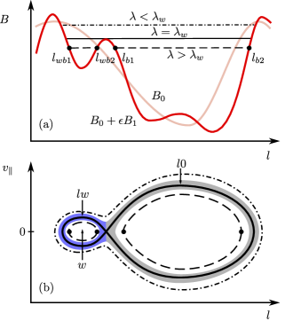
Figure 1: (a) Omnigeneous magnetic field $B_{0}$ as a function of $l$ (light), plus deviation from omnigeneity $\epsilon B_{1}$ (dark). (b) Particle orbits for $B=B_{0}+\epsilon B_{1}$ in $v_{||}$ vs. $l$ space.

Small ripple wells. Small ripple wells like the ones shown in Fig. 1(a) can form when $L\nabla\ln B_{1}\sim\epsilon^{-1}$ because it is possible to have points at which $\partial_{l}B_{0}+\epsilon\partial_{l}B_{1}=0$. The calculation so far has ignored these ripple wells. They turn out to be unimportant for the scaling.

Ripple wells affect three small regions in phase space, depicted in Fig. 1(b): the well $w$, and the layers $lw$ and $l0$. The characteristic size of these regions is given in Table 1. Ripple trapped particles in $w$ move across flux surfaces to get to the flux surface of interest. Via pitch angle diffusion, these particles can go into the layer $lw$, and moving along the magnetic field line, particles can then go into the layer $l0$. From both $lw$ and $l0$, particles can pitch angle scatter into other regions in phase space. As a result, there is a flux of particles leaving from $\lambda_{w}$, causing a discontinuity in the partial derivative $\partial_{\lambda}h_{i,t}$ at $\lambda_{w}$. By integrating in $l$ and $\lambda$ over regions $w$, $lw$ and $l0$, we can explicitly calculate the discontinuity in terms of the parameters of the ripple well parra14 . The size of the jump can be estimated from the characteristic $\Delta\lambda$ and $\Delta h_{i}$ of $l0$ (see Table 1). The jump in $\partial_{\lambda}h_{i,t}$ is of order $\epsilon\partial_{\lambda}h_{i,t}$. Even though this jump is small, in general we have a number of wells of order $\epsilon^{-1}$ in a given magnetic field line, and by accumulation, the effect of this jump condition modifies the distribution function $h_{i,t}$ by an amount of order one.

We now explain how to find the results in Table 1 parra14 . The widths of the intervals in $\lambda$ are small (the width in $v_{||}$ of the regions sketched in Fig. 1(b) is $\Delta v_{||}\sim v_{||}B_{0}\Delta\lambda$). As a result, $\partial_{\lambda}$ is large, and the pitch angle scattering piece dominates in the collision operator, $C_{ii}^{(\ell)}[h_{i}]\simeq(\nu_{\lambda}v_{||}/Bv^{2})\partial_{\lambda}\left(\lambda v_{||}\partial_{\lambda}h_{i}\right)$. The frequency $\nu_{\lambda}(v)$ is the pitch angle scattering frequency. The width of the well $w$ is $\Delta\lambda\sim\epsilon/B_{0}$ because $v_{||}=\sigma v\sqrt{1-\lambda B}$ must vanish for the range of values of $B$ in the ripple well. To estimate the change in the distribution function $\Delta h_{i}$ in the well $w$, we integrate an equation like (2) in the well. To find the widths $\Delta\lambda$ of the layers $lw$ and $l0$ we make collisions and parallel streaming comparable, and to estimate the changes in the distribution functions $\Delta h_{i}$ we impose continuity of derivatives between the well $w$ and the layer $lw$, and continuity of particle flow in phase space between the layers $lw$ and $l0$.

Table 1: Characteristic quantities in the regions in phase space that are affected by a small ripple well: parallel velocity $v_{||}$, length $\Delta l$, width of the interval in $\lambda$, $\Delta\lambda$, relative importance of collisions with respect to the parallel streaming $C_{ii}^{(\ell)}/v_{||}\partial_{l}$, and change of the distribution function within the layer $\Delta h_{i}$.

Region	$v_{||}/v_{ti}$	$\Delta l/L$	$B_{0}\Delta\lambda$	$C_{ii}^{(\ell)}/v_{||}\partial_{l}$	$\Delta h_{i}/h_{i,t}$
Well $w$	$\epsilon^{1/2}$	$\epsilon$	$\epsilon$	$\epsilon^{-1/2}\nu_{\ast}$	$\epsilon^{1/2}$
Layer $lw$	$\epsilon^{1/2}$	$\epsilon$	$\epsilon^{3/4}\nu_{\ast}^{1/2}$	$1$	$\epsilon^{1/4}\nu_{\ast}^{1/2}$
Layer $l0$	$1$	$1$	$\nu_{\ast}^{1/2}$	$1$	$\epsilon\nu_{\ast}^{1/2}$

Note that the change in the distribution function across regions $w$, $lw$ and $l0$ are small compared to $h_{i,t}$. Then, in these regions $h_{i}$ is almost constant and of order $h_{i,t}\sim\epsilon^{1/2}\nu_{\ast}^{-1}\rho_{\ast}f_{Mi}$. The number of particles in the well and its surroundings is not controlled by the well itself, but by collisional balance with the particles trapped in the larger wells.

With these estimates, we can find the contribution from the ripple wells to the energy flux. Using (1) and (5), the contribution due to the region $w$ is $Q_{i,w}\sim B_{0}\Delta\lambda\Delta\alpha(\Delta l/L)(h_{i,t}/f_{Mi})(v_{ti}/v_{||})p_{i}v_{Mi,r}S_{r}\sim\epsilon^{3}\nu_{\ast}^{-1}\rho_{\ast}^{2}p_{i}v_{ti}S_{r}$, where $\Delta\alpha\sim\epsilon$ is the extent of the well in $\alpha$, and we have neglected $\Delta h_{i}$ with respect to $h_{i,t}$. When $\epsilon^{-1/2}\nu_{\ast}\gg 1$, the small change $\Delta h_{i}$ in the layers $lw$ and $l0$ matters. The contributions from $lw$ and $l0$ are $Q_{i,lw}=O(\epsilon^{3}\rho_{\ast}^{2}p_{i}v_{ti}S_{r})$ and $Q_{i,l0}=O(\epsilon^{5/2}\rho_{\ast}^{2}p_{i}v_{ti}S_{r})$. According to these estimates, $Q_{i,lw}$ is always negligible because it is smaller than both $Q_{i,w}$ or $Q_{i,l0}$. For $\epsilon^{-1/2}\nu_{\ast}\ll 1$, $Q_{i,w}$ is larger than $Q_{i,l0}$, whereas for $\epsilon^{-1/2}\nu_{\ast}\gg 1$, $Q_{i,l0}$ is the dominant contribution. The final effect of the ripple wells depends on the total number of them. In general, we expect a number of ripple wells of order $\epsilon^{-1}$ in each magnetic field line, and the number of lines with ripple wells is of order $\epsilon^{-1}$, giving a number of wells of order $\epsilon^{-2}$. Thus, for $\epsilon^{-1/2}\nu_{\ast}\ll 1$, the total energy flux due to ripple wells is $O(\epsilon\nu_{\ast}^{-1}\rho_{\ast}^{2}p_{i}v_{ti}S_{r})$, and for $\epsilon^{-1/2}\nu_{\ast}\gg 1$, the flux due to ripple wells is $O(\epsilon^{1/2}\rho_{\ast}^{2}p_{i}v_{ti}S_{r})$. If we compare these estimates to the perfectly omnigeneous flux in (10), we find that the energy flux due to deviations from omnigeneity is higher than the flux of a perfectly omnigeneous stellarator by $A\sim\epsilon\nu_{\ast}^{-2}$ for $\epsilon^{-1/2}\nu_{\ast}\ll 1$, but it is smaller for $\epsilon^{-1/2}\nu_{\ast}\gg 1$. These estimates are exactly the same as the ones we obtained without ripple wells.

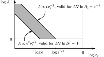
Figure 2: Energy flux amplification due to deviations from omnigeneity as function of $\nu_{\ast}$. When the deviation from omnigeneity gives flux smaller than the flux of a perfectly omnigeneous stellarator, we set the amplification to $1$.

Perturbation to omnigeneity with small gradients. To bound the effect of deviations from omnigeneity, we consider $L\nabla\ln B_{1}\sim 1$. We have evaluated the corrections to the second adiabatic invariant due to deviations from omnigeneity, $J^{(2)}$ and $J^{(3)}$, in (13) and (When omnigeneity fails). For small gradients, the size of $J^{(3)}$ is not $\epsilon^{3/2}v_{ti}L$. In the first integral in (When omnigeneity fails), we can Taylor expand $B_{0}$ and $B_{1}$ around $l_{b1}$, finding $\sqrt{1-\lambda B-\epsilon\lambda B_{1}}\simeq\sqrt{-\lambda(\partial_{l}B_{0}+\epsilon\partial_{l}B_{1})(l-l_{b1})}$ and $\sqrt{1-\lambda B_{0}}\simeq\sqrt{-\lambda\partial_{l}B_{0}(l-l_{b1})}$. Similarly, in the second integral of (When omnigeneity fails), we can Taylor expand $B_{0}$ and $B_{1}$ around $l_{b2}$. With these Taylor expansions, it is easy to see that $J^{(3)}$ is of order $\epsilon^{2}v_{ti}L$. Then, $\partial_{\alpha}J\simeq\partial_{\alpha}J^{(2)}$, and since $\partial_{\alpha}\ln B_{1}\sim 1$, $\partial_{\alpha}J\sim\epsilon v_{ti}L$. As a result, an equation similar to (12) gives $h_{i,t}\sim\epsilon\nu_{\ast}^{-1}\rho_{\ast}f_{Mi}$, and equation (15) leads to

$$Q_{i}=O(\epsilon^{2}\nu_{\ast}^{-1}\rho_{\ast}^{2}p_{i}v_{ti}S_{r}).$$ (17)

Comparing (17) with (10), we find that the amplification factor is $A\sim\epsilon^{2}\nu_{\ast}^{-2}$ for $\epsilon^{-1}\nu_{\ast}\ll 1$, and $A=1$ for $\epsilon^{-1}\nu_{\ast}\gg 1$.

There are no ripple wells formed by a perturbation with $L\nabla\ln B_{1}\sim 1$, but the addition of the perturbation $\epsilon B_{1}$ changes the height and position of the minima and maxima. This effect is studied in calvo13 for stellarators close to quasisymmetry, where it is shown to be a higher order effect. The estimation for stellarators close to omnigeneity is very similar, and gives the same result.

Conclusions. We summarize our results in Fig. 2 where we sketch the dependence on $\nu_{\ast}$ of the amplification of the energy flux $A$ due to deviations from omnigeneity.

For deviations with large gradients, the amplification is considerable at small collisionalities $\nu_{\ast}\ll\epsilon^{1/2}$. In this regime the transport is dominated by particles trapped in the wells of the omnigeneous piece of the magnetic field. Importantly, ripple wells are not crucial for this type of transport, as has sometimes been assumed. This assumption is usually based on the incorrect impression that seminal work like ho87 applies to stellarators close to omnigeneity. Unlike in ho87 , the number of particles in ripple wells is not small because these particles do not have in general small $v_{||}$. The particles that get into ripple wells by collisions come from a population that has $v_{||}\sim v_{ti}$. This is the reason why, when we assume an $O(\epsilon^{-2})$ number of wells, we obtain the flux $\epsilon\nu_{\ast}^{-1}\rho_{\ast}^{2}p_{i}v_{ti}S_{r}$ instead of $\epsilon^{3/2}\nu_{\ast}^{-1}\rho_{\ast}^{2}p_{i}v_{ti}S_{r}$.

Surprisingly, due to the large gradients associated with the deviations from omnigeneity, the energy flux is unlikely to depend quadratically on the deviations from omnigeneity even for relatively small deviations. The dependence will be between linear and quadratic, and this fact will necessarily affect the competition between different optimization criteria.