\RS@ifundefined
subref
\newref subname = section
\RS@ifundefined thmref
\newref thmname = theorem
\RS@ifundefined lemref
\newref lemname = lemma
\newref secname = \RSsectxt ,
names = \RSsecstxt ,
Name = \RSSectxt ,
Names = \RSSecstxt ,
refcmd = LABEL:#1 ,
rngtxt = \RSrngtxt ,
lsttwotxt = \RSlsttwotxt ,
lsttxt = \RSlsttxt
\newref thm
name = theorem ,
names = theorems ,
Name = Theorem ,
Names = Theorems ,
rngtxt = \RSrngtxt ,
lsttwotxt = \RSlsttxt ,
lsttxt = \RSlsttxt
\newref prop
name = proposition ,
names = propositions ,
Name = Proposition ,
Names = Propositions ,
rngtxt = \RSrngtxt ,
lsttwotxt = \RSlsttxt ,
lsttxt = \RSlsttxt
\newref cor
name = corollary ,
names = corollaries ,
Name = Corollary ,
Names = Corollaries ,
rngtxt = \RSrngtxt ,
lsttwotxt = \RSlsttxt ,
lsttxt = \RSlsttxt
\newref rem
name = remark ,
names = remarks ,
Name = Remark ,
Names = Remarks ,
rngtxt = \RSrngtxt ,
lsttwotxt = \RSlsttxt ,
lsttxt = \RSlsttxt
\newref ex
name = example ,
names = examples ,
Name = Example ,
Names = Examples ,
rngtxt = \RSrngtxt ,
lsttwotxt = \RSlsttxt ,
lsttxt = \RSlsttxt
\newref def
name = definition ,
names = definitions ,
Name = Definition ,
Names = Definitions ,
rngtxt = \RSrngtxt ,
lsttwotxt = \RSlsttxt ,
lsttxt = \RSlsttxt
Frames and Factorization of Graph Laplacians
Palle Jorgensen and Feng Tian
(Palle E.T. Jorgensen) Department of Mathematics, The University
of Iowa, Iowa City, IA 52242-1419, U.S.A.
palle-jorgensen@uiowa.edu
(Feng Tian) Department of Mathematics, Wright State University, Dayton,
OH 45435, U.S.A.
feng.tian@wright.edu
Abstract.
Using functions from electrical networks (graphs with resistors assigned
to edges), we prove existence (with explicit formulas) of a canonical
Parseval frame in the energy Hilbert space ℋ E subscript ℋ 𝐸 \mathscr{H}_{E} ℋ E subscript ℋ 𝐸 \mathscr{H}_{E} ℋ E subscript ℋ 𝐸 \mathscr{H}_{E}
We consider infinite connected network-graphs G = ( V , E ) 𝐺 𝑉 𝐸 G=\left(V,E\right) V 𝑉 V E for edges. To every conductance function
c 𝑐 c E 𝐸 E G 𝐺 G ( ℋ E , Δ ) subscript ℋ 𝐸 Δ \left(\mathscr{H}_{E},\Delta\right) ℋ E subscript ℋ 𝐸 \mathscr{H}_{E} Δ ( = Δ c ) annotated Δ absent subscript Δ 𝑐 \Delta\left(=\Delta_{c}\right) c 𝑐 c c 𝑐 c ℋ E subscript ℋ 𝐸 \mathscr{H}_{E} Δ Δ \Delta l 2 ( V ) superscript 𝑙 2 𝑉 l^{2}\left(V\right) ℋ E subscript ℋ 𝐸 \mathscr{H}_{E} l 2 ( V ) superscript 𝑙 2 𝑉 l^{2}\left(V\right) ℋ E subscript ℋ 𝐸 \mathscr{H}_{E} ℋ E subscript ℋ 𝐸 \mathscr{H}_{E} l 2 ( V ) superscript 𝑙 2 𝑉 l^{2}\left(V\right)
Key words and phrases:
Unbounded operators, deficiency-indices, Hilbert space, boundary
values, weighted graph, reproducing kernel, Dirichlet form, graph
Laplacian, resistance network, harmonic analysis, frame, Parseval
frame, Friedrichs extension, reversible random walk, resistance distance,
energy Hilbert space.
2000 Mathematics Subject Classification:
Primary 47L60, 46N30, 46N50, 42C15, 65R10, 05C50, 05C75, 31C20; Secondary
46N20, 22E70, 31A15, 58J65, 81S25
Contents
1 Introduction2 Basic Setting
3 Electrical Current as Frame Coefficients
3.1 Dipoles
4 Lemmas5 The Hilbert Spaces ℋ E subscript ℋ 𝐸 \mathscr{H}_{E} l 2 ( V ′ ) superscript 𝑙 2 superscript 𝑉 ′ l^{2}\left(V^{\prime}\right)
6 The Friedrichs Extension
6.1 The operator P 𝑃 P Δ Δ \Delta
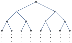
7 Examples
7.1 V = { 0 } ∪ ℤ + 𝑉 0 subscript ℤ V=\left\{0\right\}\cup\mathbb{Z}_{+} 7.2 A reversible walk on the binary tree (the binomial
model)7.3 A 2D lattice7.4 A Parseval frame that is not an ONB in ℋ E subscript ℋ 𝐸 \mathscr{H}_{E}
8 Open problems
1. Introduction
We study infinite networks with the use of frames in Hilbert space.
While our results apply to finite systems, we will concentrate on
the infinite case because of its statistical significance.
By a network we mean a graph G 𝐺 G V 𝑉 V E 𝐸 E Δ Δ \Delta V 𝑉 V
The functions on V 𝑉 V V 𝑉 V ℋ E subscript ℋ 𝐸 \mathscr{H}_{E} ℋ E subscript ℋ 𝐸 \mathscr{H}_{E}
In our first result we identify a canonical Parseval frame in ℋ E subscript ℋ 𝐸 \mathscr{H}_{E} ℋ E subscript ℋ 𝐸 \mathscr{H}_{E} e 𝑒 e e 𝑒 e e 𝑒 e
We apply our frame to complete a number of explicit results. We study
the Friedrichs extension of the graph Laplacian Δ Δ \Delta ℋ E subscript ℋ 𝐸 \mathscr{H}_{E} Δ Δ \Delta
Continuing earlier work [Jor08 , JP13 , JP11a , JP11b , JP10 , MS14 , Fol14 ]
on analysis and spectral theory of infinite connected network-graphs
G = ( V , E ) 𝐺 𝑉 𝐸 G=\left(V,E\right) V 𝑉 V E 𝐸 E c 𝑐 c G 𝐺 G c 𝑐 c E 𝐸 E G 𝐺 G ( ℋ E , Δ ) subscript ℋ 𝐸 Δ \left(\mathscr{H}_{E},\Delta\right) ℋ E subscript ℋ 𝐸 \mathscr{H}_{E} Δ ( = Δ c ) annotated Δ absent subscript Δ 𝑐 \Delta\left(=\Delta_{c}\right) c 𝑐 c c 𝑐 c [AJSV13 , JS12 , CJ12b , CJ12a , JP12 , Dur06 , ST81 , Ter78 ]
and the papers cited there.
It is also known that Δ Δ \Delta l 2 ( V ) superscript 𝑙 2 𝑉 l^{2}\left(V\right) ℋ E subscript ℋ 𝐸 \mathscr{H}_{E} [JP10 ] . As an l 2 ( V ) superscript 𝑙 2 𝑉 l^{2}\left(V\right) Δ Δ \Delta ∞ × ∞ \infty\times\infty ( c , G ) 𝑐 𝐺 \left(c,G\right) Δ Δ \Delta l 2 ( V ) superscript 𝑙 2 𝑉 l^{2}\left(V\right) ℋ E subscript ℋ 𝐸 \mathscr{H}_{E} [Jor08 , JP13 ] .
Hence as an ℋ E subscript ℋ 𝐸 \mathscr{H}_{E} ℋ E subscript ℋ 𝐸 \mathscr{H}_{E} l 2 ( V ) superscript 𝑙 2 𝑉 l^{2}\left(V\right)
We begin with the basic notions needed, and we then turn to our theorem
about Parseval frames: In 3 ℋ E subscript ℋ 𝐸 \mathscr{H}_{E}
2. Basic Setting
Overview of the details below: The graph Laplacian Δ Δ \Delta 2.2 l 2 ( V ) superscript 𝑙 2 𝑉 l^{2}\left(V\right) 2.3 { δ x } subscript 𝛿 𝑥 \left\{\delta_{x}\right\} l 2 ( V ) superscript 𝑙 2 𝑉 l^{2}(V) l 2 ( V ) superscript 𝑙 2 𝑉 l^{2}(V) ℋ E subscript ℋ 𝐸 \mathscr{H}_{E} 3.2
The problem with this is that there is not an independent characterization
of the domain d o m ( Δ , ℋ E ) 𝑑 𝑜 𝑚 Δ subscript ℋ 𝐸 dom\left(\Delta,\mathscr{H}_{E}\right) Δ Δ \Delta ℋ E subscript ℋ 𝐸 \mathscr{H}_{E} l 2 ( V ) superscript 𝑙 2 𝑉 l^{2}(V) 4.1 𝒟 E subscript 𝒟 𝐸 \mathscr{D}_{E} V 𝑉 V ℋ E subscript ℋ 𝐸 \mathscr{H}_{E} ℋ E subscript ℋ 𝐸 \mathscr{H}_{E} V 𝑉 V Δ Δ \Delta ℋ E subscript ℋ 𝐸 \mathscr{H}_{E} 3.4 { δ x } subscript 𝛿 𝑥 \left\{\delta_{x}\right\} l 2 ( V ) superscript 𝑙 2 𝑉 l^{2}(V) ℋ E subscript ℋ 𝐸 \mathscr{H}_{E} ℋ E subscript ℋ 𝐸 \mathscr{H}_{E} { δ x } subscript 𝛿 𝑥 \left\{\delta_{x}\right\} ℋ E subscript ℋ 𝐸 \mathscr{H}_{E} ℋ E subscript ℋ 𝐸 \mathscr{H}_{E}
Let V 𝑉 V E ⊂ V × V 𝐸 𝑉 𝑉 E\subset V\times V
(1)
( x , y ) ∈ E ⟺ ( y , x ) ∈ E ⟺ 𝑥 𝑦 𝐸 𝑦 𝑥 𝐸 \left(x,y\right)\in E\Longleftrightarrow\left(y,x\right)\in E x , y ∈ V 𝑥 𝑦
𝑉 x,y\in V
(2)
# { y ∈ V | ( x , y ) ∈ E } # conditional-set 𝑦 𝑉 𝑥 𝑦 𝐸 \#\left\{y\in V\>|\>\left(x,y\right)\in E\right\} > 0 absent 0 >0 x ∈ V 𝑥 𝑉 x\in V
(3)
( x , x ) ∉ E 𝑥 𝑥 𝐸 \left(x,x\right)\notin E
(4)
∃ o ∈ V 𝑜 𝑉 \exists\,o\in V y ∈ V 𝑦 𝑉 y\in V ∃ x 0 , x 1 , … , x n ∈ V subscript 𝑥 0 subscript 𝑥 1 … subscript 𝑥 𝑛
𝑉 \exists\,x_{0},x_{1},\ldots,x_{n}\in V x 0 = o subscript 𝑥 0 𝑜 x_{0}=o x n = y subscript 𝑥 𝑛 𝑦 x_{n}=y ( x i − 1 , x i ) ∈ E subscript 𝑥 𝑖 1 subscript 𝑥 𝑖 𝐸 \left(x_{i-1},x_{i}\right)\in E ∀ i = 1 , … , n for-all 𝑖 1 … 𝑛
\forall i=1,\ldots,n
If a conductance function c 𝑐 c c x i − 1 x i > 0 subscript 𝑐 subscript 𝑥 𝑖 1 subscript 𝑥 𝑖 0 c_{x_{i-1}x_{i}}>0
Definition 2.1 .
A function c : E → ℝ + ∪ { 0 } : 𝑐 → 𝐸 subscript ℝ 0 c:E\rightarrow\mathbb{R}_{+}\cup\left\{0\right\} conductance function if c ( e ) ≥ 0 𝑐 𝑒 0 c\left(e\right)\geq 0 ∀ e ∈ E for-all 𝑒 𝐸 \forall e\in E x ∈ V 𝑥 𝑉 x\in V ( x , y ) ∈ E 𝑥 𝑦 𝐸 \left(x,y\right)\in E c x y > 0 subscript 𝑐 𝑥 𝑦 0 c_{xy}>0 c x y = c y x subscript 𝑐 𝑥 𝑦 subscript 𝑐 𝑦 𝑥 c_{xy}=c_{yx}
Notation: If x ∈ V 𝑥 𝑉 x\in V
c ( x ) := ∑ y c x y , sum over { y ∈ V | ( x , y ) ∈ E } := E ( x ) . assign 𝑐 𝑥 subscript 𝑦 subscript 𝑐 𝑥 𝑦 sum over { y ∈ V | ( x , y ) ∈ E } := E ( x ) .
c\left(x\right):=\sum_{y}c_{xy},\>\mbox{sum over $\left\{y\in V\>\big{|}\>\left(x,y\right)\in E\right\}:=E\left(x\right)$.} (2.1)
The summation in (2.1 x ∼ y similar-to 𝑥 𝑦 x\sim y x ∼ y similar-to 𝑥 𝑦 x\sim y ( x , y ) ∈ E 𝑥 𝑦 𝐸 \left(x,y\right)\in E
Definition 2.2 .
When c 𝑐 c 2.1 Δ = Δ c Δ subscript Δ 𝑐 \Delta=\Delta_{c}
( Δ u ) ( x ) Δ 𝑢 𝑥 \displaystyle\left(\Delta u\right)\left(x\right) = ∑ y ∼ x c x y ( u ( x ) − u ( y ) ) absent subscript similar-to 𝑦 𝑥 subscript 𝑐 𝑥 𝑦 𝑢 𝑥 𝑢 𝑦 \displaystyle=\sum_{y\sim x}c_{xy}\left(u\left(x\right)-u\left(y\right)\right) (2.2)
= c ( x ) u ( x ) − ∑ y ∼ x c x y u ( y ) . absent 𝑐 𝑥 𝑢 𝑥 subscript similar-to 𝑦 𝑥 subscript 𝑐 𝑥 𝑦 𝑢 𝑦 \displaystyle=c\left(x\right)u\left(x\right)-\sum_{y\sim x}c_{xy}u\left(y\right).
Remark 2.3 .
Given ( V , E , c ) 𝑉 𝐸 𝑐 \left(V,E,c\right) Δ = Δ c Δ subscript Δ 𝑐 \Delta=\Delta_{c} V 𝑉 V ∞ × ∞ \infty\times\infty Δ Δ \Delta
[ c ( x 1 ) − c x 1 x 2 0 ⋯ ⋯ ⋯ ⋯ 0 ⋯ − c x 2 x 1 c ( x 2 ) − c x 2 x 3 0 ⋯ ⋯ ⋯ ⋮ ⋯ 0 − c x 3 x 2 c ( x 3 ) − c x 3 x 4 0 ⋯ ⋯ 0 ⋯ ⋮ 0 ⋱ ⋱ ⋱ ⋱ ⋮ ⋮ ⋯ ⋮ ⋮ ⋱ ⋱ ⋱ ⋱ 0 ⋮ ⋯ ⋮ 0 ⋯ 0 − c x n x n − 1 c ( x n ) − c x n x n + 1 0 ⋯ ⋮ ⋮ ⋯ ⋯ 0 ⋱ ⋱ ⋱ ⋱ ] matrix 𝑐 subscript 𝑥 1 subscript 𝑐 subscript 𝑥 1 subscript 𝑥 2 0 ⋯ ⋯ ⋯ ⋯ 0 ⋯ subscript 𝑐 subscript 𝑥 2 subscript 𝑥 1 𝑐 subscript 𝑥 2 subscript 𝑐 subscript 𝑥 2 subscript 𝑥 3 0 ⋯ ⋯ ⋯ ⋮ ⋯ 0 subscript 𝑐 subscript 𝑥 3 subscript 𝑥 2 𝑐 subscript 𝑥 3 subscript 𝑐 subscript 𝑥 3 subscript 𝑥 4 0 ⋯ ⋯ 0 ⋯ ⋮ 0 ⋱ ⋱ ⋱ ⋱ ⋮ ⋮ ⋯ ⋮ ⋮ ⋱ ⋱ ⋱ ⋱ 0 ⋮ ⋯ ⋮ 0 ⋯ 0 subscript 𝑐 subscript 𝑥 𝑛 subscript 𝑥 𝑛 1 𝑐 subscript 𝑥 𝑛 subscript 𝑐 subscript 𝑥 𝑛 subscript 𝑥 𝑛 1 0 ⋯ ⋮ ⋮ ⋯ ⋯ 0 ⋱ ⋱ ⋱ ⋱ \begin{bmatrix}c\left(x_{1}\right)&-c_{x_{1}x_{2}}&0&\cdots&\cdots&\cdots&\cdots&0&\cdots\\
-c_{x_{2}x_{1}}&c\left(x_{2}\right)&-c_{x_{2}x_{3}}&0&\cdots&\cdots&\cdots&\vdots&\cdots\\
0&-c_{x_{3}x_{2}}&c\left(x_{3}\right)&-c_{x_{3}x_{4}}&0&\cdots&\cdots&\huge\mbox{0}&\cdots\\
\vdots&0&\ddots&\ddots&\ddots&\ddots&\vdots&\vdots&\cdots\\
\vdots&\vdots&\ddots&\ddots&\ddots&\ddots&0&\vdots&\cdots\\
\vdots&\huge\mbox{0}&\cdots&0&-c_{x_{n}x_{n-1}}&c\left(x_{n}\right)&-c_{x_{n}x_{n+1}}&0&\cdots\\
\vdots&\vdots&\cdots&\cdots&0&\ddots&\ddots&\ddots&\ddots\end{bmatrix} (2.3)
(We refer to [GLS12 ] for a number of applications of infinite
banded matrices.)
If # E ( x ) = 2 # 𝐸 𝑥 2 \#E\left(x\right)=2 x ∈ V 𝑥 𝑉 x\in V E ( x ) := { y ∈ V | ( x , y ) ∈ E } assign 𝐸 𝑥 conditional-set 𝑦 𝑉 𝑥 𝑦 𝐸 E\left(x\right):=\left\{y\in V\>|\>\left(x,y\right)\in E\right\} ( V , E , c ) 𝑉 𝐸 𝑐 \left(V,E,c\right) V 𝑉 V
o 𝑜 \textstyle{o\ignorespaces\ignorespaces\ignorespaces\ignorespaces\ignorespaces} c o x 1 subscript 𝑐 𝑜 subscript 𝑥 1 \scriptstyle{c_{ox_{1}}} x 1 subscript 𝑥 1 \textstyle{x_{1}\ignorespaces\ignorespaces\ignorespaces\ignorespaces\ignorespaces} c x 1 x 2 subscript 𝑐 subscript 𝑥 1 subscript 𝑥 2 \scriptstyle{c_{x_{1}x_{2}}} x 2 subscript 𝑥 2 \textstyle{x_{2}} ⋯ ⋯ \textstyle{\cdots} x n − 1 subscript 𝑥 𝑛 1 \textstyle{x_{n-1}\ignorespaces\ignorespaces\ignorespaces\ignorespaces\ignorespaces} c x n − 1 x n subscript 𝑐 subscript 𝑥 𝑛 1 subscript 𝑥 𝑛 \scriptstyle{c_{x_{n-1}x_{n}}} x n subscript 𝑥 𝑛 \textstyle{x_{n}\ignorespaces\ignorespaces\ignorespaces\ignorespaces\ignorespaces} c x n x n + 1 subscript 𝑐 subscript 𝑥 𝑛 subscript 𝑥 𝑛 1 \scriptstyle{c_{x_{n}x_{n+1}}} x n + 1 ⋯ subscript 𝑥 𝑛 1 ⋯ \textstyle{x_{n+1}\cdots} (2.4)
[ c ( o ) − c o x 1 0 ⋯ ⋯ ⋯ 0 − c o x 1 c ( x 1 ) − c x 1 x 2 0 ⋯ ⋯ ⋮ 0 − c x 1 x 2 c ( x 2 ) c x 2 x 3 0 0 ⋮ ⋱ ⋱ ⋱ ⋱ ⋱ ⋮ ⋮ ⋯ ⋱ − c x n x n − 1 c ( x n ) − c x n x n + 1 0 ⋮ ⋯ ⋱ ⋱ ⋱ ⋱ 0 ⋯ ⋯ ⋯ 0 ] matrix 𝑐 𝑜 subscript 𝑐 𝑜 subscript 𝑥 1 0 ⋯ ⋯ ⋯ 0 subscript 𝑐 𝑜 subscript 𝑥 1 𝑐 subscript 𝑥 1 subscript 𝑐 subscript 𝑥 1 subscript 𝑥 2 0 ⋯ ⋯ ⋮ 0 subscript 𝑐 subscript 𝑥 1 subscript 𝑥 2 𝑐 subscript 𝑥 2 subscript 𝑐 subscript 𝑥 2 subscript 𝑥 3 0 missing-subexpression 0 ⋮ ⋱ ⋱ ⋱ ⋱ ⋱ ⋮ ⋮ ⋯ ⋱ subscript 𝑐 subscript 𝑥 𝑛 subscript 𝑥 𝑛 1 𝑐 subscript 𝑥 𝑛 subscript 𝑐 subscript 𝑥 𝑛 subscript 𝑥 𝑛 1 0 ⋮ ⋯ missing-subexpression ⋱ ⋱ ⋱ ⋱ 0 ⋯ ⋯ ⋯ 0 \begin{bmatrix}c\left(o\right)&-c_{ox_{1}}&0&\cdots&\cdots&\cdots&0\\
-c_{ox_{1}}&c\left(x_{1}\right)&-c_{x_{1}x_{2}}&0&\cdots&\cdots&\vdots\\
0&-c_{x_{1}x_{2}}&c\left(x_{2}\right)&c_{x_{2}x_{3}}&0&&\huge\mbox{0}\\
\vdots&\ddots&\ddots&\ddots&\ddots&\ddots&\vdots\\
\vdots&\cdots&\ddots&-c_{x_{n}x_{n-1}}&c\left(x_{n}\right)&-c_{x_{n}x_{n+1}}&0\\
\vdots&\cdots&&\ddots&\ddots&\ddots&\ddots\\
\huge\mbox{0}&\cdots&\cdots&\cdots&0\end{bmatrix} (2.5)
Remark 2.4 (Random Walk ).
If ( V , E , c ) 𝑉 𝐸 𝑐 \left(V,E,c\right) 2.2 ( x , y ) ∈ E 𝑥 𝑦 𝐸 \left(x,y\right)\in E
p x y := c x y c ( x ) assign subscript 𝑝 𝑥 𝑦 subscript 𝑐 𝑥 𝑦 𝑐 𝑥 p_{xy}:=\frac{c_{xy}}{c\left(x\right)} (2.6)
and note then { p x y } subscript 𝑝 𝑥 𝑦 \left\{p_{xy}\right\} 2.6 ∑ y p x y = 1 subscript 𝑦 subscript 𝑝 𝑥 𝑦 1 \sum_{y}p_{xy}=1 ∀ x ∈ V for-all 𝑥 𝑉 \forall x\in V 2.1
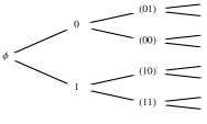
Figure 2.1. Transition probabilities p x y subscript 𝑝 𝑥 𝑦 p_{xy} x 𝑥 x ( in V ) in 𝑉 \left(\mbox{in }V\right)
A Markov-random walk on V 𝑉 V ( p x y ) subscript 𝑝 𝑥 𝑦 \left(p_{xy}\right) reversible iff ∃ \exists c ~ ~ 𝑐 \widetilde{c} V 𝑉 V
c ~ ( x ) p x y = c ~ ( y ) p y x , ∀ ( x y ) ∈ E . formulae-sequence ~ 𝑐 𝑥 subscript 𝑝 𝑥 𝑦 ~ 𝑐 𝑦 subscript 𝑝 𝑦 𝑥 for-all 𝑥 𝑦 𝐸 \widetilde{c}\left(x\right)p_{xy}=\widetilde{c}\left(y\right)p_{yx},\;\forall\left(xy\right)\in E. (2.7)
Lemma 2.5 .
There is a bijective correspondence between reversible Markov-walks
on the one hand, and conductance functions on the other.
Proof.
If c 𝑐 c E 𝐸 E 2.1 ( p x y ) subscript 𝑝 𝑥 𝑦 \left(p_{xy}\right) 2.6 c x y = c y x subscript 𝑐 𝑥 𝑦 subscript 𝑐 𝑦 𝑥 c_{xy}=c_{yx}
Conversely if (2.7 ( p x y = Prob ( x ↦ y ) ) subscript 𝑝 𝑥 𝑦 Prob maps-to 𝑥 𝑦 \left(p_{xy}=\mbox{Prob}\left(x\mapsto y\right)\right) c x y := c ~ ( x ) p x y assign subscript 𝑐 𝑥 𝑦 ~ 𝑐 𝑥 subscript 𝑝 𝑥 𝑦 c_{xy}:=\widetilde{c}\left(x\right)p_{xy}
c ~ ( x ) = ∑ y ∼ x c x y . ~ 𝑐 𝑥 subscript similar-to 𝑦 𝑥 subscript 𝑐 𝑥 𝑦 \widetilde{c}\left(x\right)=\sum_{y\sim x}c_{xy}.
For results on reversible Markov chains, see e.g., [LPP12 ] .
3. Electrical Current as Frame Coefficients
The role of the graph-network setting ( V , E , c , ℋ E ) 𝑉 𝐸 𝑐 subscript ℋ 𝐸 \left(V,E,c,\mathscr{H}_{E}\right) G 𝐺 G V 𝑉 V E 𝐸 E V 𝑉 V G 𝐺 G v ( x , y ) subscript 𝑣 𝑥 𝑦 v_{\left(x,y\right)} ℋ E subscript ℋ 𝐸 \mathscr{H}_{E} x 𝑥 x y 𝑦 y c 𝑐 c x 𝑥 x y 𝑦 y ( V , E , c ) 𝑉 𝐸 𝑐 \left(V,E,c\right) v x y subscript 𝑣 𝑥 𝑦 v_{xy} not in l 2 ( V ) superscript 𝑙 2 𝑉 l^{2}\left(V\right) ℋ E subscript ℋ 𝐸 \mathscr{H}_{E} 3.4
For a fixed function u 𝑢 u ℋ E subscript ℋ 𝐸 \mathscr{H}_{E} e 𝑒 e E 𝐸 E I ( u , e ) 𝐼 𝑢 𝑒 I\left(u,e\right) frame coefficients in a
natural Parseval frame (for ℋ E subscript ℋ 𝐸 \mathscr{H}_{E} v e subscript 𝑣 𝑒 v_{e} e = ( x , y ) 𝑒 𝑥 𝑦 e=\left(x,y\right) E 𝐸 E
This result will be proved below. For general background references
on frames in Hilbert space, we refer to [HJL+ , KLZ09 , CM13 , SD13 , KOPT13 , EO13 ] ,
and for electrical networks, see [Ana11 , Gri10 , Zem96 , Bar93 , Tet91 , DS84 , NW59 ] .
The facts on electrical networks we need are the laws of Kirchhoff
and Ohm, and our computation of the frame coefficients as electrical
currents is based on this, in part.
Definition 3.1 .
Let ℋ ℋ \mathscr{H} ⟨ ⋅ , ⋅ ⟩ ⋅ ⋅
\left\langle\cdot,\cdot\right\rangle ⟨ ⋅ , ⋅ ⟩ ℋ subscript ⋅ ⋅
ℋ \left\langle\cdot,\cdot\right\rangle_{\mathscr{H}} J 𝐽 J { w j } j ∈ J subscript subscript 𝑤 𝑗 𝑗 𝐽 \left\{w_{j}\right\}_{j\in J} ℋ ℋ \mathscr{H} { w j } j ∈ J subscript subscript 𝑤 𝑗 𝑗 𝐽 \left\{w_{j}\right\}_{j\in J} frame for ℋ ℋ \mathscr{H} b 1 subscript 𝑏 1 b_{1} b 2 subscript 𝑏 2 b_{2}
b 1 ‖ u ‖ ℋ 2 ≤ ∑ j ∈ J | ⟨ w j , u ⟩ ℋ | 2 ≤ b 2 ‖ u ‖ ℋ 2 subscript 𝑏 1 superscript subscript norm 𝑢 ℋ 2 subscript 𝑗 𝐽 superscript subscript subscript 𝑤 𝑗 𝑢
ℋ 2 subscript 𝑏 2 superscript subscript norm 𝑢 ℋ 2 b_{1}\left\|u\right\|_{\mathscr{H}}^{2}\leq\sum_{j\in J}\left|\left\langle w_{j},u\right\rangle_{\mathscr{H}}\right|^{2}\leq b_{2}\left\|u\right\|_{\mathscr{H}}^{2} (3.1)
holds for all u ∈ ℋ 𝑢 ℋ u\in\mathscr{H} Parseval
frame if b 1 = b 2 = 1 subscript 𝑏 1 subscript 𝑏 2 1 b_{1}=b_{2}=1
Lemma 3.2 .
If { w j } j ∈ J subscript subscript 𝑤 𝑗 𝑗 𝐽 \left\{w_{j}\right\}_{j\in J} ℋ ℋ \mathscr{H} A = A ℋ : ℋ ⟶ l 2 ( J ) : 𝐴 subscript 𝐴 ℋ ⟶ ℋ superscript 𝑙 2 𝐽 A=A_{\mathscr{H}}:\mathscr{H}\longrightarrow l^{2}\left(J\right)
A u = ( ⟨ w j , u ⟩ ℋ ) j ∈ J 𝐴 𝑢 subscript subscript subscript 𝑤 𝑗 𝑢
ℋ 𝑗 𝐽 Au=\left(\left\langle w_{j},u\right\rangle_{\mathscr{H}}\right)_{j\in J} (3.2)
is well-defined and isometric. Its adjoint A ∗ : l 2 ( J ) ⟶ ℋ : superscript 𝐴 ⟶ superscript 𝑙 2 𝐽 ℋ A^{*}:l^{2}\left(J\right)\longrightarrow\mathscr{H}
A ∗ ( ( γ j ) j ∈ J ) := ∑ j ∈ J γ j w j assign superscript 𝐴 subscript subscript 𝛾 𝑗 𝑗 𝐽 subscript 𝑗 𝐽 subscript 𝛾 𝑗 subscript 𝑤 𝑗 A^{*}\left(\left(\gamma_{j}\right)_{j\in J}\right):=\sum_{j\in J}\gamma_{j}w_{j} (3.3)
and the following hold:
(1)
The sum on the RHS in ( 3.3 ) is norm-convergent;
(2)
A ∗ : l 2 ( J ) ⟶ ℋ : superscript 𝐴 ⟶ superscript 𝑙 2 𝐽 ℋ A^{*}:l^{2}\left(J\right)\longrightarrow\mathscr{H} is co-isometric;
and for all u ∈ ℋ 𝑢 ℋ u\in\mathscr{H} , we have
u = A ∗ A u = ∑ j ∈ J ⟨ w j , u ⟩ w j 𝑢 superscript 𝐴 𝐴 𝑢 subscript 𝑗 𝐽 subscript 𝑤 𝑗 𝑢
subscript 𝑤 𝑗 u=A^{*}Au=\sum_{j\in J}\left\langle w_{j},u\right\rangle w_{j} (3.4)
where the RHS in ( 3.4 ) is norm-convergent.
Proof.
The details are standard in the theory of frames; see the cited papers
above. Note that (3.1 b 1 = b 2 = 1 subscript 𝑏 1 subscript 𝑏 2 1 b_{1}=b_{2}=1 A 𝐴 A 3.2 A ∗ A = I ℋ = superscript 𝐴 𝐴 subscript 𝐼 ℋ absent A^{*}A=I_{\mathscr{H}}= ℋ ℋ \mathscr{H} A A ∗ = 𝐴 superscript 𝐴 absent AA^{*}= A 𝐴 A
When a conductance function c : E → ℝ + ∪ { 0 } : 𝑐 → 𝐸 subscript ℝ 0 c:E\rightarrow\mathbb{R}_{+}\cup\left\{0\right\} ℋ E subscript ℋ 𝐸 \mathscr{H}_{E} c 𝑐 c
⟨ u , v ⟩ ℋ E subscript 𝑢 𝑣
subscript ℋ 𝐸 \displaystyle\left\langle u,v\right\rangle_{\mathscr{H}_{E}} := 1 2 ∑ ∑ ( x , y ) ∈ E c x y ( u ( x ) ¯ − u ( y ) ¯ ) ( v ( x ) − v ( y ) ) , and assign absent 1 2 𝑥 𝑦 𝐸 subscript 𝑐 𝑥 𝑦 ¯ 𝑢 𝑥 ¯ 𝑢 𝑦 𝑣 𝑥 𝑣 𝑦 and
\displaystyle:=\frac{1}{2}\underset{\left(x,y\right)\in E}{\sum\sum}c_{xy}\left(\overline{u\left(x\right)}-\overline{u\left(y\right)}\right)\left(v\left(x\right)-v\left(y\right)\right),\mbox{ and} (3.5)
‖ u ‖ ℋ E 2 superscript subscript norm 𝑢 subscript ℋ 𝐸 2 \displaystyle\left\|u\right\|_{\mathscr{H}_{E}}^{2} = ⟨ u , u ⟩ ℋ E = 1 2 ∑ ∑ ( x , y ) ∈ E c x y | u ( x ) − u ( y ) | 2 < ∞ . absent subscript 𝑢 𝑢
subscript ℋ 𝐸 1 2 𝑥 𝑦 𝐸 subscript 𝑐 𝑥 𝑦 superscript 𝑢 𝑥 𝑢 𝑦 2 \displaystyle=\left\langle u,u\right\rangle_{\mathscr{H}_{E}}=\frac{1}{2}\underset{\left(x,y\right)\in E}{\sum\sum}c_{xy}\left|u\left(x\right)-u\left(y\right)\right|^{2}<\infty. (3.6)
We shall assume that ( V , E , c ) 𝑉 𝐸 𝑐 \left(V,E,c\right) connected
(See Definition 2.1 3.4 3.5 ℋ E subscript ℋ 𝐸 \mathscr{H}_{E} V 𝑉 V 4
Further, for any pair of vertices x , y ∈ V 𝑥 𝑦
𝑉 x,y\in V v x y ∈ ℋ E subscript 𝑣 𝑥 𝑦 subscript ℋ 𝐸 v_{xy}\in\mathscr{H}_{E}
⟨ v x y , u ⟩ ℋ E = u ( x ) − u ( y ) subscript subscript 𝑣 𝑥 𝑦 𝑢
subscript ℋ 𝐸 𝑢 𝑥 𝑢 𝑦 \left\langle v_{xy},u\right\rangle_{\mathscr{H}_{E}}=u\left(x\right)-u\left(y\right) (3.7)
holds for all u ∈ ℋ E 𝑢 subscript ℋ 𝐸 u\in\mathscr{H}_{E} 3.4
Remark 3.3 .
We illustrate this Parseval frame in section 7.4
3.1. Dipoles
Let ( V , E , c , ℋ E ) 𝑉 𝐸 𝑐 subscript ℋ 𝐸 \left(V,E,c,\mathscr{H}_{E}\right) ( V , E , c ) 𝑉 𝐸 𝑐 \left(V,E,c\right) ℋ E subscript ℋ 𝐸 \mathscr{H}_{E} V 𝑉 V G = ( V , E ) 𝐺 𝑉 𝐸 G=\left(V,E\right)
Lemma 3.4 ([JP10 ] ).
For every pair of vertices x , y ∈ V 𝑥 𝑦
𝑉 x,y\in V unique vector v x y ∈ ℋ E subscript 𝑣 𝑥 𝑦 subscript ℋ 𝐸 v_{xy}\in\mathscr{H}_{E}
⟨ u , v x y ⟩ ℋ E = u ( x ) − u ( y ) subscript 𝑢 subscript 𝑣 𝑥 𝑦
subscript ℋ 𝐸 𝑢 𝑥 𝑢 𝑦 \left\langle u,v_{xy}\right\rangle_{\mathscr{H}_{E}}=u\left(x\right)-u\left(y\right) (3.8)
for all u ∈ ℋ E 𝑢 subscript ℋ 𝐸 u\in\mathscr{H}_{E}
Proof.
Fix a pair of vertices x , y 𝑥 𝑦
x,y ( x i , x i + 1 ) ∈ E subscript 𝑥 𝑖 subscript 𝑥 𝑖 1 𝐸 \left(x_{i},x_{i+1}\right)\in E c x i , x i + 1 > 0 subscript 𝑐 subscript 𝑥 𝑖 subscript 𝑥 𝑖 1
0 c_{x_{i},x_{i+1}}>0 x 0 = y subscript 𝑥 0 𝑦 x_{0}=y x n = x subscript 𝑥 𝑛 𝑥 x_{n}=x
u ( x ) − u ( y ) 𝑢 𝑥 𝑢 𝑦 \displaystyle u\left(x\right)-u\left(y\right) = ∑ i = 0 n − 1 u ( x i + 1 ) − u ( x i ) absent superscript subscript 𝑖 0 𝑛 1 𝑢 subscript 𝑥 𝑖 1 𝑢 subscript 𝑥 𝑖 \displaystyle=\sum_{i=0}^{n-1}u\left(x_{i+1}\right)-u\left(x_{i}\right)
= ∑ i = 0 n − 1 1 c x i x i + 1 c x i x i + 1 ( u ( x i + 1 ) − u ( x i ) ) ; absent superscript subscript 𝑖 0 𝑛 1 1 subscript 𝑐 subscript 𝑥 𝑖 subscript 𝑥 𝑖 1 subscript 𝑐 subscript 𝑥 𝑖 subscript 𝑥 𝑖 1 𝑢 subscript 𝑥 𝑖 1 𝑢 subscript 𝑥 𝑖 \displaystyle=\sum_{i=0}^{n-1}\frac{1}{\sqrt{c_{x_{i}x_{i+1}}}}\sqrt{c_{x_{i}x_{i+1}}}\left(u\left(x_{i+1}\right)-u\left(x_{i}\right)\right); (3.9)
and, by Schwarz, we have the following estimate:
| u ( x ) − u ( y ) | 2 superscript 𝑢 𝑥 𝑢 𝑦 2 \displaystyle\left|u\left(x\right)-u\left(y\right)\right|^{2} ≤ ( ∑ i = 0 n − 1 1 c x i x i + 1 ) ∑ j = 0 n − 1 c x j x j + 1 | u ( x j + 1 ) − u ( x j ) | 2 absent superscript subscript 𝑖 0 𝑛 1 1 subscript 𝑐 subscript 𝑥 𝑖 subscript 𝑥 𝑖 1 superscript subscript 𝑗 0 𝑛 1 subscript 𝑐 subscript 𝑥 𝑗 subscript 𝑥 𝑗 1 superscript 𝑢 subscript 𝑥 𝑗 1 𝑢 subscript 𝑥 𝑗 2 \displaystyle\leq\left(\sum_{i=0}^{n-1}\frac{1}{c_{x_{i}x_{i+1}}}\right)\sum_{j=0}^{n-1}c_{x_{j}x_{j+1}}\left|u\left(x_{j+1}\right)-u\left(x_{j}\right)\right|^{2}
≤ ( Const x y ) ‖ u ‖ ℋ E 2 , absent subscript Const 𝑥 𝑦 superscript subscript norm 𝑢 subscript ℋ 𝐸 2 \displaystyle\leq\left(\mbox{Const}_{xy}\right)\left\|u\right\|_{\mathscr{H}_{E}}^{2},
valid for all u ∈ ℋ E 𝑢 subscript ℋ 𝐸 u\in\mathscr{H}_{E} 3.6 a priori estimate. But this states
that the linear functional:
L x y : ℋ E ∋ u ⟼ u ( x ) − u ( y ) : subscript 𝐿 𝑥 𝑦 contains subscript ℋ 𝐸 𝑢 ⟼ 𝑢 𝑥 𝑢 𝑦 L_{xy}:\mathscr{H}_{E}\ni u\longmapsto u\left(x\right)-u\left(y\right) (3.10)
is continuous on ℋ E subscript ℋ 𝐸 \mathscr{H}_{E} ∥ ⋅ ∥ ℋ E \left\|\cdot\right\|_{\mathscr{H}_{E}} v x y ∈ ℋ E subscript 𝑣 𝑥 𝑦 subscript ℋ 𝐸 v_{xy}\in\mathscr{H}_{E} ∃ ! v x y ∈ ℋ E subscript 𝑣 𝑥 𝑦 subscript ℋ 𝐸 \exists!v_{xy}\in\mathscr{H}_{E}
L x y ( u ) = ⟨ v x y , u ⟩ ℋ E , ∀ u ∈ ℋ E . formulae-sequence subscript 𝐿 𝑥 𝑦 𝑢 subscript subscript 𝑣 𝑥 𝑦 𝑢
subscript ℋ 𝐸 for-all 𝑢 subscript ℋ 𝐸 L_{xy}\left(u\right)=\left\langle v_{xy},u\right\rangle_{\mathscr{H}_{E}},\;\forall u\in\mathscr{H}_{E}.
∎
Remark 3.5 .
Let x , y ∈ V 𝑥 𝑦
𝑉 x,y\in V v x y ∈ ℋ E subscript 𝑣 𝑥 𝑦 subscript ℋ 𝐸 v_{xy}\in\mathscr{H}_{E} 2.1 2.2
Δ v x y = δ x − δ y . Δ subscript 𝑣 𝑥 𝑦 subscript 𝛿 𝑥 subscript 𝛿 𝑦 \Delta v_{xy}=\delta_{x}-\delta_{y}. (3.11)
But this equation (3.11 not determine v x y subscript 𝑣 𝑥 𝑦 v_{xy} w 𝑤 w V 𝑉 V Δ w = 0 Δ 𝑤 0 \Delta w=0 w 𝑤 w harmonic , then v x y + w subscript 𝑣 𝑥 𝑦 𝑤 v_{xy}+w 3.11 [JP11a , JP11b ] we studied when ( V , E , c ) 𝑉 𝐸 𝑐 \left(V,E,c\right) ℋ E subscript ℋ 𝐸 \mathscr{H}_{E}
The system of vectors v x y subscript 𝑣 𝑥 𝑦 v_{xy} 3.7 ( V , E , c , ℋ E ) 𝑉 𝐸 𝑐 subscript ℋ 𝐸 \left(V,E,c,\mathscr{H}_{E}\right) resistance metric .
Lemma 3.6 .
When c 𝑐 c ( V , c ) 𝑉 𝑐 \left(V,c\right)
d c ( x , y ) := sup { 1 ‖ u ‖ ℋ E 2 | u ∈ ℋ E , u ( x ) = 1 , u ( y ) = 0 } assign subscript 𝑑 𝑐 𝑥 𝑦 supremum conditional-set 1 superscript subscript norm 𝑢 subscript ℋ 𝐸 2 formulae-sequence 𝑢 subscript ℋ 𝐸 formulae-sequence 𝑢 𝑥 1 𝑢 𝑦 0 d_{c}\left(x,y\right):=\sup\left\{\frac{1}{\left\|u\right\|_{\mathscr{H}_{E}}^{2}}\>\Big{|}\>u\in\mathscr{H}_{E},u\left(x\right)=1,u\left(y\right)=0\right\} (3.12)
then d c ( x , y ) subscript 𝑑 𝑐 𝑥 𝑦 d_{c}\left(x,y\right) V 𝑉 V
d c ( x , y ) = ‖ v x y ‖ ℋ E 2 subscript 𝑑 𝑐 𝑥 𝑦 superscript subscript norm subscript 𝑣 𝑥 𝑦 subscript ℋ 𝐸 2 d_{c}\left(x,y\right)=\left\|v_{xy}\right\|_{\mathscr{H}_{E}}^{2} (3.13)
where the dipole vectors are specified as in (3.7
Proof.
Consider u ∈ ℋ E 𝑢 subscript ℋ 𝐸 u\in\mathscr{H}_{E} 3.12 u ( x ) = 1 𝑢 𝑥 1 u\left(x\right)=1 u ( y ) = 0 𝑢 𝑦 0 u\left(y\right)=0 3.7
1 1 \displaystyle 1 = u ( x ) − u ( y ) = | ⟨ v x y , u ⟩ ℋ E | 2 absent 𝑢 𝑥 𝑢 𝑦 superscript subscript subscript 𝑣 𝑥 𝑦 𝑢
subscript ℋ 𝐸 2 \displaystyle=u\left(x\right)-u\left(y\right)=\left|\left\langle v_{xy},u\right\rangle_{\mathscr{H}_{E}}\right|^{2}
≤ ‖ v x y ‖ ℋ E 2 ‖ u ‖ ℋ E 2 . ( by Schwarz ) formulae-sequence absent superscript subscript norm subscript 𝑣 𝑥 𝑦 subscript ℋ 𝐸 2 superscript subscript norm 𝑢 subscript ℋ 𝐸 2 by Schwarz \displaystyle\leq\left\|v_{xy}\right\|_{\mathscr{H}_{E}}^{2}\left\|u\right\|_{\mathscr{H}_{E}}^{2}.\;\left(\mbox{by Schwarz}\right)
Since we know the optimizing vectors in the Schwarz inequality, the
desired formula (3.13 3.12 3.7
But (3.12
The next lemma offers a lower bound for the resistance metric between
any two vertices when ( V , E , c ) 𝑉 𝐸 𝑐 \left(V,E,c\right) x 𝑥 x y 𝑦 y dist c ( x , y ) ≥ subscript dist 𝑐 𝑥 𝑦 absent \mbox{dist}_{c}\left(x,y\right)\geq x 𝑥 x y 𝑦 y
Lemma 3.7 .
Let G = ( V , E , c ) 𝐺 𝑉 𝐸 𝑐 G=\left(V,E,c\right) x 0 := x → ( e i ) → x n := y assign subscript 𝑥 0 𝑥 → subscript 𝑒 𝑖 → subscript 𝑥 𝑛 assign 𝑦 x_{0}:=x\rightarrow\left(e_{i}\right)\rightarrow x_{n}:=y
dist c ( x , y ) ≥ ∑ i = 0 n − 1 Res x i x i + 1 | I ( v x y ) i , i + 1 | 2 ⏟ dissipation ; subscript dist 𝑐 𝑥 𝑦 dissipation ⏟ superscript subscript 𝑖 0 𝑛 1 subscript Res subscript 𝑥 𝑖 subscript 𝑥 𝑖 1 superscript 𝐼 subscript subscript 𝑣 𝑥 𝑦 𝑖 𝑖 1
2 \mbox{dist}_{c}\left(x,y\right)\geq\underset{\mbox{dissipation}}{\underbrace{\sum_{i=0}^{n-1}\mbox{Res}_{x_{i}x_{i+1}}\left|I\left(v_{xy}\right)_{i,i+1}\right|^{2}}}; (3.14)
where Res = 1 c Res 1 𝑐 \mbox{Res}=\frac{1}{c}
Proof.
In general there are many paths from x 𝑥 x y 𝑦 y x 𝑥 x y 𝑦 y 3.1
‖ v x y ‖ ℋ E 2 superscript subscript norm subscript 𝑣 𝑥 𝑦 subscript ℋ 𝐸 2 \displaystyle\left\|v_{xy}\right\|_{\mathscr{H}_{E}}^{2} = dist c ( x , y ) = ∑ e ∈ E ( d i r ) | ⟨ w e , v x y ⟩ ℋ E | 2 ( w e := c e v e ) formulae-sequence absent subscript dist 𝑐 𝑥 𝑦 subscript 𝑒 superscript 𝐸 𝑑 𝑖 𝑟 superscript subscript subscript 𝑤 𝑒 subscript 𝑣 𝑥 𝑦
subscript ℋ 𝐸 2 assign subscript 𝑤 𝑒 subscript 𝑐 𝑒 subscript 𝑣 𝑒 \displaystyle=\mbox{dist}_{c}\left(x,y\right)=\sum_{e\in E^{\left(dir\right)}}\left|\left\langle w_{e},v_{xy}\right\rangle_{\mathscr{H}_{E}}\right|^{2}\quad\left(w_{e}:=\sqrt{c_{e}}v_{e}\right)
= ∑ e ∈ E ( d i r ) c c | ⟨ v e , v x y ⟩ ℋ E | 2 absent subscript 𝑒 superscript 𝐸 𝑑 𝑖 𝑟 subscript 𝑐 𝑐 superscript subscript subscript 𝑣 𝑒 subscript 𝑣 𝑥 𝑦
subscript ℋ 𝐸 2 \displaystyle=\sum_{e\in E^{\left(dir\right)}}c_{c}\left|\left\langle v_{e},v_{xy}\right\rangle_{\mathscr{H}_{E}}\right|^{2}
≥ ∑ i = 0 n − 1 c i , i + 1 | v x y ( x i ) − v x y ( x i + 1 ) | 2 absent superscript subscript 𝑖 0 𝑛 1 subscript 𝑐 𝑖 𝑖 1
superscript subscript 𝑣 𝑥 𝑦 subscript 𝑥 𝑖 subscript 𝑣 𝑥 𝑦 subscript 𝑥 𝑖 1 2 \displaystyle\geq\sum_{i=0}^{n-1}c_{i,i+1}\left|v_{xy}\left(x_{i}\right)-v_{xy}\left(x_{i+1}\right)\right|^{2}
= ∑ i = 0 n − 1 Res x i x i + 1 | I ( v x y ) x i x i + 1 | 2 . absent superscript subscript 𝑖 0 𝑛 1 subscript Res subscript 𝑥 𝑖 subscript 𝑥 𝑖 1 superscript 𝐼 subscript subscript 𝑣 𝑥 𝑦 subscript 𝑥 𝑖 subscript 𝑥 𝑖 1 2 \displaystyle=\sum_{i=0}^{n-1}\mbox{Res}_{x_{i}x_{i+1}}\left|I\left(v_{xy}\right)_{x_{i}x_{i+1}}\right|^{2}.
Figure 3.1. Two finite paths connecting x 𝑥 x y 𝑦 y e i = ( x i x i + 1 ) , e j ~ = ( x ~ j x ~ j + 1 ) ∈ E formulae-sequence subscript 𝑒 𝑖 subscript 𝑥 𝑖 subscript 𝑥 𝑖 1 ~ subscript 𝑒 𝑗 subscript ~ 𝑥 𝑗 subscript ~ 𝑥 𝑗 1 𝐸 e_{i}=\left(x_{i}x_{i+1}\right),\widetilde{e_{j}}=\left(\widetilde{x}_{j}\widetilde{x}_{j+1}\right)\in E
Now pick an orientation for each edge, and denote by E ( o r i ) superscript 𝐸 𝑜 𝑟 𝑖 E^{\left(ori\right)}
Theorem 3.8 .
Let ( V , E , c , E ( o r i ) ) 𝑉 𝐸 𝑐 superscript 𝐸 𝑜 𝑟 𝑖 \left(V,E,c,E^{\left(ori\right)}\right) ℋ E subscript ℋ 𝐸 \mathscr{H}_{E}
w x y := c x y v x y , indexed by ( x y ) ∈ E ( o r i ) assign subscript 𝑤 𝑥 𝑦 subscript 𝑐 𝑥 𝑦 subscript 𝑣 𝑥 𝑦 indexed by ( x y ) ∈ E ( o r i )
w_{xy}:=\sqrt{c_{xy}}v_{xy},\;\mbox{indexed by $\left(xy\right)\in E^{\left(ori\right)}$} (3.15)
is a Parseval frame for ℋ E subscript ℋ 𝐸 \mathscr{H}_{E}
Proof.
We will show that (3.1 b 1 = b 2 = 1 subscript 𝑏 1 subscript 𝑏 2 1 b_{1}=b_{2}=1 ( w ( x y ) ) ( x y ) ∈ E ( o r i ) subscript subscript 𝑤 𝑥 𝑦 𝑥 𝑦 superscript 𝐸 𝑜 𝑟 𝑖 \left(w_{\left(xy\right)}\right)_{\left(xy\right)\in E^{\left(ori\right)}} 3.7 3.15
Indeed we have for u ∈ ℋ E 𝑢 subscript ℋ 𝐸 u\in\mathscr{H}_{E}
‖ u ‖ ℋ E 2 superscript subscript norm 𝑢 subscript ℋ 𝐸 2 \displaystyle\left\|u\right\|_{\mathscr{H}_{E}}^{2} = ( by ( 3.6 ) ) by ( 3.6 ) \displaystyle\underset{\left(\text{by $\left(\ref{eq:en6}\right)$}\right)}{=} ∑ ( x y ) ∈ E ( o r i ) c x y | u ( x ) − u ( y ) | 2 subscript 𝑥 𝑦 superscript 𝐸 𝑜 𝑟 𝑖 subscript 𝑐 𝑥 𝑦 superscript 𝑢 𝑥 𝑢 𝑦 2 \displaystyle\sum_{\left(xy\right)\in E^{\left(ori\right)}}c_{xy}\left|u\left(x\right)-u\left(y\right)\right|^{2}
= ( by ( 3.7 ) ) by ( 3.7 ) \displaystyle\underset{\left(\text{by $\left(\ref{eq:en7}\right)$}\right)}{=} ∑ ( x y ) ∈ E ( o r i ) c x y | ⟨ v x y , u ⟩ ℋ E | 2 subscript 𝑥 𝑦 superscript 𝐸 𝑜 𝑟 𝑖 subscript 𝑐 𝑥 𝑦 superscript subscript subscript 𝑣 𝑥 𝑦 𝑢
subscript ℋ 𝐸 2 \displaystyle\sum_{\left(xy\right)\in E^{\left(ori\right)}}c_{xy}\left|\left\langle v_{xy},u\right\rangle_{\mathscr{H}_{E}}\right|^{2}
= \displaystyle= ∑ ( x y ) ∈ E ( o r i ) | ⟨ c x y v x y , u ⟩ ℋ E | 2 subscript 𝑥 𝑦 superscript 𝐸 𝑜 𝑟 𝑖 superscript subscript subscript 𝑐 𝑥 𝑦 subscript 𝑣 𝑥 𝑦 𝑢
subscript ℋ 𝐸 2 \displaystyle\sum_{\left(xy\right)\in E^{\left(ori\right)}}\left|\left\langle\sqrt{c_{xy}}v_{xy},u\right\rangle_{\mathscr{H}_{E}}\right|^{2}
= ( by ( 3.15 ) ) by ( 3.15 ) \displaystyle\underset{\left(\text{by $\left(\ref{eq:en8}\right)$}\right)}{=} ∑ ( x y ) ∈ E ( o r i ) | ⟨ w x y , u ⟩ ℋ E | 2 subscript 𝑥 𝑦 superscript 𝐸 𝑜 𝑟 𝑖 superscript subscript subscript 𝑤 𝑥 𝑦 𝑢
subscript ℋ 𝐸 2 \displaystyle\sum_{\left(xy\right)\in E^{\left(ori\right)}}\left|\left\langle w_{xy},u\right\rangle_{\mathscr{H}_{E}}\right|^{2}
which is the desired conclusion.∎
Remark 3.9 .
While the vectors w x y := c x y v x y assign subscript 𝑤 𝑥 𝑦 subscript 𝑐 𝑥 𝑦 subscript 𝑣 𝑥 𝑦 w_{xy}:=\sqrt{c_{xy}}v_{xy} ( x y ) ∈ E ( o r i ) 𝑥 𝑦 superscript 𝐸 𝑜 𝑟 𝑖 \left(xy\right)\in E^{\left(ori\right)} ℋ E subscript ℋ 𝐸 \mathscr{H}_{E} ℋ E subscript ℋ 𝐸 \mathscr{H}_{E} 7.1
To see when our Parseval frames are in fact ONBs, we use the following:
Lemma 3.10 .
Let { w j } j ∈ J subscript subscript 𝑤 𝑗 𝑗 𝐽 \left\{w_{j}\right\}_{j\in J} ℋ ℋ \mathscr{H} ‖ w j ‖ ℋ E ≤ 1 subscript norm subscript 𝑤 𝑗 subscript ℋ 𝐸 1 \left\|w_{j}\right\|_{\mathscr{H}_{E}}\leq 1 ℋ ℋ \mathscr{H} ‖ w j ‖ ℋ = 1 subscript norm subscript 𝑤 𝑗 ℋ 1 \left\|w_{j}\right\|_{\mathscr{H}}=1 j ∈ J 𝑗 𝐽 j\in J
Proof.
Follows from an easy application of
‖ u ‖ ℋ 2 = ∑ j ∈ J | ⟨ w j , u ⟩ ℋ | 2 , u ∈ ℋ . formulae-sequence superscript subscript norm 𝑢 ℋ 2 subscript 𝑗 𝐽 superscript subscript subscript 𝑤 𝑗 𝑢
ℋ 2 𝑢 ℋ \left\|u\right\|_{\mathscr{H}}^{2}=\sum_{j\in J}\left|\left\langle w_{j},u\right\rangle_{\mathscr{H}}\right|^{2},\;u\in\mathscr{H}. (3.16)
Plug in w j 0 subscript 𝑤 subscript 𝑗 0 w_{j_{0}} u 𝑢 u 3.16
Remark 3.11 .
Frames in ℋ E subscript ℋ 𝐸 \mathscr{H}_{E} 3.15 3.2 7.4
V = Band 𝑉 Band V=\mbox{Band}
V = ℤ 2 𝑉 superscript ℤ 2 V=\mathbb{Z}^{2}
Figure 3.2. non-linear system of vertices
In these examples one checks that
1 > ‖ w x y ‖ ℋ E 2 = c x y ‖ v x y ‖ ℋ E 2 = c x y ( v x y ( x ) − v x y ( y ) ) . 1 superscript subscript norm subscript 𝑤 𝑥 𝑦 subscript ℋ 𝐸 2 subscript 𝑐 𝑥 𝑦 superscript subscript norm subscript 𝑣 𝑥 𝑦 subscript ℋ 𝐸 2 subscript 𝑐 𝑥 𝑦 subscript 𝑣 𝑥 𝑦 𝑥 subscript 𝑣 𝑥 𝑦 𝑦 1>\left\|w_{xy}\right\|_{\mathscr{H}_{E}}^{2}=c_{xy}\left\|v_{xy}\right\|_{\mathscr{H}_{E}}^{2}=c_{xy}\left(v_{xy}\left(x\right)-v_{xy}\left(y\right)\right). (3.17)
That is the current flowing through each edge e = ( x , y ) ∈ E 𝑒 𝑥 𝑦 𝐸 e=\left(x,y\right)\in E < 1 absent 1 <1 e 𝑒 e < <
v x y ( x ) − v x y ( y ) < 1 c c y = resistance. subscript 𝑣 𝑥 𝑦 𝑥 subscript 𝑣 𝑥 𝑦 𝑦 1 subscript 𝑐 𝑐 𝑦 resistance. v_{xy}\left(x\right)-v_{xy}\left(y\right)<\frac{1}{c_{cy}}=\mbox{resistance.}
Definition 3.12 .
Let V , E , c , ℋ E 𝑉 𝐸 𝑐 subscript ℋ 𝐸
V,E,c,\mathscr{H}_{E} u ∈ ℋ E 𝑢 subscript ℋ 𝐸 u\in\mathscr{H}_{E}
I ( u ) ( x y ) := c x y ( u ( x ) − u ( y ) ) for ( x , y ) ∈ E . assign 𝐼 subscript 𝑢 𝑥 𝑦 subscript 𝑐 𝑥 𝑦 𝑢 𝑥 𝑢 𝑦 for ( x , y ) ∈ E I\left(u\right)_{\left(xy\right)}:=c_{xy}\left(u\left(x\right)-u\left(y\right)\right)\;\mbox{for $\left(x,y\right)\in E$}. (3.18)
By Ohm’s law, the function I ( u ) ( x y ) 𝐼 subscript 𝑢 𝑥 𝑦 I\left(u\right)_{\left(xy\right)} 3.18
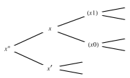
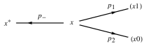
A choice of orientation may be assigned as follows
(three different ways):
(1)
The orientation of every ( x y ) ∈ E 𝑥 𝑦 𝐸 \left(xy\right)\in E
(2)
The orientation may be suggested by geometry; for example in a binary
tree, as shown in Fig 3.3
(3)
Or the orientation may be assigned by the experiment
of inserting one Amp at a vertex, say o ∈ V 𝑜 𝑉 o\in V x d i s t ∈ V subscript 𝑥 𝑑 𝑖 𝑠 𝑡 𝑉 x_{dist}\in V ( x y ) ∈ E 𝑥 𝑦 𝐸 \left(xy\right)\in E I ( u ) x y > 0 𝐼 subscript 𝑢 𝑥 𝑦 0 I\left(u\right)_{xy}>0 I ( u ) x y 𝐼 subscript 𝑢 𝑥 𝑦 I\left(u\right)_{xy} 3.18 3.4
Figure 3.3. Geometric orientation. (See also Fig 7.4 Figure 3.4. Electrically induced orientation.
Corollary 3.13 .
Let ( V , E , c , ℋ E ) 𝑉 𝐸 𝑐 subscript ℋ 𝐸 \left(V,E,c,\mathscr{H}_{E}\right) E ( o r i ) superscript 𝐸 𝑜 𝑟 𝑖 E^{\left(ori\right)} 3 3.12 u ∈ ℋ E 𝑢 subscript ℋ 𝐸 u\in\mathscr{H}_{E}
u = ∑ ( x y ) ∈ E ( o r i ) I ( u ) x y v x y . 𝑢 subscript 𝑥 𝑦 superscript 𝐸 𝑜 𝑟 𝑖 𝐼 subscript 𝑢 𝑥 𝑦 subscript 𝑣 𝑥 𝑦 u=\sum_{\left(xy\right)\in E^{\left(ori\right)}}I\left(u\right)_{xy}v_{xy}. (3.19)
Proof.
By Theorem 3.8 3.2
u = ∑ ( x y ) ∈ E ( o r i ) ⟨ w x y , u ⟩ ℋ E w x y , 𝑢 subscript 𝑥 𝑦 superscript 𝐸 𝑜 𝑟 𝑖 subscript subscript 𝑤 𝑥 𝑦 𝑢
subscript ℋ 𝐸 subscript 𝑤 𝑥 𝑦 u=\sum_{\left(xy\right)\in E^{\left(ori\right)}}\left\langle w_{xy},u\right\rangle_{\mathscr{H}_{E}}w_{xy}, (3.20)
see (3.4 3.15 3.18
⟨ w x y , u ⟩ ℋ E w x y = I ( u ) x y v x y . subscript subscript 𝑤 𝑥 𝑦 𝑢
subscript ℋ 𝐸 subscript 𝑤 𝑥 𝑦 𝐼 subscript 𝑢 𝑥 𝑦 subscript 𝑣 𝑥 𝑦 \left\langle w_{xy},u\right\rangle_{\mathscr{H}_{E}}w_{xy}=I\left(u\right)_{xy}v_{xy}. (3.21)
Considering (3.20 3.21 3.19
4. Lemmas
Starting with a given network ( V , E , c ) 𝑉 𝐸 𝑐 (V,E,c) V 𝑉 V E 𝐸 E Δ Δ \Delta P 𝑃 P l 2 ( V ) superscript 𝑙 2 𝑉 l^{2}(V) ℋ E subscript ℋ 𝐸 \mathscr{H}_{E} c 𝑐 c
Lemma 4.2 Δ Δ \Delta l 2 ( V ) superscript 𝑙 2 𝑉 l^{2}(V) ℋ E subscript ℋ 𝐸 \mathscr{H}_{E} ( V , E , c ) 𝑉 𝐸 𝑐 (V,E,c) ℋ E subscript ℋ 𝐸 \mathscr{H}_{E} 4.3 l 2 ( V ) superscript 𝑙 2 𝑉 l^{2}(V)
Recall that the graph-Laplacian Δ Δ \Delta l 2 ( V ) superscript 𝑙 2 𝑉 l^{2}(V) ℋ E subscript ℋ 𝐸 \mathscr{H}_{E} [Jor08 , JP11b ] . In section
7 ( Δ , ℋ E ) Δ subscript ℋ 𝐸 (\Delta,\mathscr{H}_{E}) ( m , m ) 𝑚 𝑚 (m,m) m > 0 𝑚 0 m>0 P 𝑃 P
Let ( V , E , c ) 𝑉 𝐸 𝑐 \left(V,E,c\right) G = ( V , E ) 𝐺 𝑉 𝐸 G=\left(V,E\right) o 𝑜 o V 𝑉 V x ∈ V 𝑥 𝑉 x\in V o 𝑜 o V ′ := V \ { o } assign superscript 𝑉 ′ \ 𝑉 𝑜 V^{\prime}:=V\backslash\left\{o\right\} l 2 ( V ) superscript 𝑙 2 𝑉 l^{2}\left(V\right) l 2 ( V ′ ) superscript 𝑙 2 superscript 𝑉 ′ l^{2}\left(V^{\prime}\right) x ∈ V 𝑥 𝑉 x\in V
δ x ( y ) = { 1 if y = x 0 if y ≠ x subscript 𝛿 𝑥 𝑦 cases 1 if 𝑦 𝑥 0 if 𝑦 𝑥 \delta_{x}\left(y\right)=\begin{cases}1&\mbox{if }y=x\\
0&\mbox{if }y\neq x\end{cases} (4.1)
Set ℋ E := assign subscript ℋ 𝐸 absent \mathscr{H}_{E}:= u : V → ℂ : 𝑢 → 𝑉 ℂ u:V\rightarrow\mathbb{C}
‖ u ‖ ℋ E 2 := 1 2 ∑ ∑ ( x , y ) ∈ E c x y | u ( x ) − u ( y ) | 2 < ∞ , assign superscript subscript norm 𝑢 subscript ℋ 𝐸 2 1 2 𝑥 𝑦 𝐸 subscript 𝑐 𝑥 𝑦 superscript 𝑢 𝑥 𝑢 𝑦 2 \left\|u\right\|_{\mathscr{H}_{E}}^{2}:=\frac{1}{2}\underset{\left(x,y\right)\in E}{\sum\sum}c_{xy}\left|u\left(x\right)-u\left(y\right)\right|^{2}<\infty, (4.2)
and we note [JP10 ] that ℋ E subscript ℋ 𝐸 \mathscr{H}_{E} x , y ∈ V 𝑥 𝑦
𝑉 x,y\in V v x y ∈ ℋ E subscript 𝑣 𝑥 𝑦 subscript ℋ 𝐸 v_{xy}\in\mathscr{H}_{E}
Δ v x , y = δ x − δ y . Δ subscript 𝑣 𝑥 𝑦
subscript 𝛿 𝑥 subscript 𝛿 𝑦 \Delta v_{x,y}=\delta_{x}-\delta_{y}. (4.3)
If y = o 𝑦 𝑜 y=o v x := v x , o assign subscript 𝑣 𝑥 subscript 𝑣 𝑥 𝑜
v_{x}:=v_{x,o}
Δ v x = δ x − δ o . Δ subscript 𝑣 𝑥 subscript 𝛿 𝑥 subscript 𝛿 𝑜 \Delta v_{x}=\delta_{x}-\delta_{o}. (4.4)
In this case, we assume that v x subscript 𝑣 𝑥 v_{x} x ∈ V ′ 𝑥 superscript 𝑉 ′ x\in V^{\prime}
Definition 4.1 .
Let ( V , E , c , o , Δ , { v x } x ∈ V ′ ) 𝑉 𝐸 𝑐 𝑜 Δ subscript subscript 𝑣 𝑥 𝑥 superscript 𝑉 ′ \left(V,E,c,o,\Delta,\left\{v_{x}\right\}_{x\in V^{\prime}}\right)
𝒟 2 subscript 𝒟 2 \displaystyle\mathscr{D}_{2} := s p a n { δ x | x ∈ V } , and assign absent 𝑠 𝑝 𝑎 𝑛 conditional-set subscript 𝛿 𝑥 𝑥 𝑉 and
\displaystyle:=span\left\{\delta_{x}\>\big{|}\>x\in V\right\},\;\mbox{and} (4.5)
𝒟 E subscript 𝒟 𝐸 \displaystyle\mathscr{D}_{E} := s p a n { v x | x ∈ V ′ } , assign absent 𝑠 𝑝 𝑎 𝑛 conditional-set subscript 𝑣 𝑥 𝑥 superscript 𝑉 ′ \displaystyle:=span\left\{v_{x}\>\big{|}\>x\in V^{\prime}\right\}, (4.6)
where by “span” we mean of all finite linear combinations.
Lemma 4.2 .
The following hold:
(1)
⟨ Δ u , v ⟩ l 2 = ⟨ u , Δ v ⟩ l 2 subscript Δ 𝑢 𝑣
superscript 𝑙 2 subscript 𝑢 Δ 𝑣
superscript 𝑙 2 \left\langle\Delta u,v\right\rangle_{l^{2}}=\left\langle u,\Delta v\right\rangle_{l^{2}} ,
∀ u , v ∈ 𝒟 2 for-all 𝑢 𝑣
subscript 𝒟 2 \forall u,v\in\mathscr{D}_{2} ;
(2)
⟨ Δ u , v ⟩ ℋ E = ⟨ u , Δ v ⟩ ℋ E , subscript Δ 𝑢 𝑣
subscript ℋ 𝐸 subscript 𝑢 Δ 𝑣
subscript ℋ 𝐸 \left\langle\Delta u,v\right\rangle_{\mathscr{H}_{E}}=\left\langle u,\Delta v\right\rangle_{\mathscr{H}_{E}},
∀ u , v ∈ 𝒟 E for-all 𝑢 𝑣
subscript 𝒟 𝐸 \forall u,v\in\mathscr{D}_{E} ;
(3)
⟨ u , Δ u ⟩ l 2 ≥ 0 subscript 𝑢 Δ 𝑢
superscript 𝑙 2 0 \left\langle u,\Delta u\right\rangle_{l^{2}}\geq 0 ,
∀ u ∈ 𝒟 2 for-all 𝑢 subscript 𝒟 2 \forall u\in\mathscr{D}_{2} , and
(4)
⟨ u , Δ u ⟩ ℋ E ≥ 0 subscript 𝑢 Δ 𝑢
subscript ℋ 𝐸 0 \left\langle u,\Delta u\right\rangle_{\mathscr{H}_{E}}\geq 0 , ∀ u ∈ 𝒟 E for-all 𝑢 subscript 𝒟 𝐸 \forall u\in\mathscr{D}_{E} ;
where for u , v ∈ ℋ E 𝑢 𝑣
subscript ℋ 𝐸 u,v\in\mathscr{H}_{E} we set
⟨ u , v ⟩ ℋ E = 1 2 ∑ ∑ ( x , y ) ∈ E c x y ( u ( x ) − u ( y ) ) ¯ ( v ( x ) − v ( y ) ) . subscript 𝑢 𝑣
subscript ℋ 𝐸 1 2 𝑥 𝑦 𝐸 subscript 𝑐 𝑥 𝑦 ¯ 𝑢 𝑥 𝑢 𝑦 𝑣 𝑥 𝑣 𝑦 \left\langle u,v\right\rangle_{\mathscr{H}_{E}}=\frac{1}{2}\underset{\left(x,y\right)\in E}{\sum\sum}c_{xy}\overline{\left(u\left(x\right)-u\left(y\right)\right)}\left(v\left(x\right)-v\left(y\right)\right). (4.7)
Moreover, we have
(5)
⟨ v x , y , u ⟩ ℋ E = u ( x ) − u ( y ) subscript subscript 𝑣 𝑥 𝑦
𝑢
subscript ℋ 𝐸 𝑢 𝑥 𝑢 𝑦 \left\langle v_{x,y},u\right\rangle_{\mathscr{H}_{E}}=u\left(x\right)-u\left(y\right) ,
∀ x , y ∈ V for-all 𝑥 𝑦
𝑉 \forall x,y\in V .
Finally,
(6)
δ x ( ⋅ ) = c ( x ) v x ( ⋅ ) − ∑ y ∼ x c x y v y ( ⋅ ) , ∀ x ∈ V ′ . formulae-sequence subscript 𝛿 𝑥 ⋅ 𝑐 𝑥 subscript 𝑣 𝑥 ⋅ subscript similar-to 𝑦 𝑥 subscript 𝑐 𝑥 𝑦 subscript 𝑣 𝑦 ⋅ for-all 𝑥 superscript 𝑉 ′ \delta_{x}\left(\cdot\right)=c\left(x\right)v_{x}\left(\cdot\right)-\sum_{y\sim x}c_{xy}v_{y}\left(\cdot\right),\;\forall x\in V^{\prime}.
Proof.
Proof of (2 We have ⟨ Δ u , v ⟩ ℋ E = ⟨ u , Δ v ⟩ ℋ E subscript Δ 𝑢 𝑣
subscript ℋ 𝐸 subscript 𝑢 Δ 𝑣
subscript ℋ 𝐸 \left\langle\Delta u,v\right\rangle_{\mathscr{H}_{E}}=\left\langle u,\Delta v\right\rangle_{\mathscr{H}_{E}} u , v ∈ 𝒟 E 𝑢 𝑣
subscript 𝒟 𝐸 u,v\in\mathscr{D}_{E} v x := v x o assign subscript 𝑣 𝑥 subscript 𝑣 𝑥 𝑜 v_{x}:=v_{xo} o 𝑜 o V 𝑉 V V ′ := V \ { o } assign superscript 𝑉 ′ \ 𝑉 𝑜 V^{\prime}:=V\backslash\left\{o\right\} Δ v x = δ x − δ o Δ subscript 𝑣 𝑥 subscript 𝛿 𝑥 subscript 𝛿 𝑜 \Delta v_{x}=\delta_{x}-\delta_{o} x ∈ V ′ 𝑥 superscript 𝑉 ′ x\in V^{\prime} u = ∑ x ∈ V ′ ξ x v x 𝑢 subscript 𝑥 superscript 𝑉 ′ subscript 𝜉 𝑥 subscript 𝑣 𝑥 u=\sum_{x\in V^{\prime}}\xi_{x}v_{x} v = ∑ x ∈ V ′ η x v x 𝑣 subscript 𝑥 superscript 𝑉 ′ subscript 𝜂 𝑥 subscript 𝑣 𝑥 v=\sum_{x\in V^{\prime}}\eta_{x}v_{x}
⟨ Δ u , v ⟩ ℋ E subscript Δ 𝑢 𝑣
subscript ℋ 𝐸 \displaystyle\left\langle\Delta u,v\right\rangle_{\mathscr{H}_{E}} = \displaystyle= ∑ V ′ ∑ V ′ ξ x ¯ η y ⟨ δ x − δ o , v y ⟩ ℋ E subscript superscript 𝑉 ′ subscript superscript 𝑉 ′ ¯ subscript 𝜉 𝑥 subscript 𝜂 𝑦 subscript subscript 𝛿 𝑥 subscript 𝛿 𝑜 subscript 𝑣 𝑦
subscript ℋ 𝐸 \displaystyle\sum_{V^{\prime}}\sum_{V^{\prime}}\overline{\xi_{x}}\eta_{y}\left\langle\delta_{x}-\delta_{o},v_{y}\right\rangle_{\mathscr{H}_{E}}
= \displaystyle= ∑ V ′ ∑ V ′ ξ x ¯ η y ( ( δ x ( y ) − δ x ( o ) ⏟ = 0 ) − ( δ o ( y ) ⏟ = 0 − δ o ( o ) ⏟ = 1 ) ) subscript superscript 𝑉 ′ subscript superscript 𝑉 ′ ¯ subscript 𝜉 𝑥 subscript 𝜂 𝑦 subscript 𝛿 𝑥 𝑦 absent 0 ⏟ subscript 𝛿 𝑥 𝑜 absent 0 ⏟ subscript 𝛿 𝑜 𝑦 absent 1 ⏟ subscript 𝛿 𝑜 𝑜 \displaystyle\sum_{V^{\prime}}\sum_{V^{\prime}}\overline{\xi_{x}}\eta_{y}\big{(}(\delta_{x}\left(y\right)-\underset{{\scriptscriptstyle=0}}{\underbrace{\delta_{x}\left(o\right)}})-(\underset{{\scriptscriptstyle=0}}{\underbrace{\delta_{o}\left(y\right)}}-\underset{{\scriptscriptstyle=1}}{\underbrace{\delta_{o}\left(o\right)}})\big{)}
= \displaystyle= ∑ V ′ ∑ V ′ ξ x ¯ η y ( δ x y + 1 ) subscript superscript 𝑉 ′ subscript superscript 𝑉 ′ ¯ subscript 𝜉 𝑥 subscript 𝜂 𝑦 subscript 𝛿 𝑥 𝑦 1 \displaystyle\sum_{V^{\prime}}\sum_{V^{\prime}}\overline{\xi_{x}}\eta_{y}\left(\delta_{xy}+1\right)
= \displaystyle= ∑ V ′ ξ x ¯ η y + ( ∑ V ′ ξ x ¯ ) ( ∑ V ′ η y ) subscript superscript 𝑉 ′ ¯ subscript 𝜉 𝑥 subscript 𝜂 𝑦 ¯ subscript superscript 𝑉 ′ subscript 𝜉 𝑥 subscript superscript 𝑉 ′ subscript 𝜂 𝑦 \displaystyle\sum_{V^{\prime}}\overline{\xi_{x}}\eta_{y}+\left(\overline{\sum_{V^{\prime}}\xi_{x}}\right)\left(\sum_{V^{\prime}}\eta_{y}\right)
= \displaystyle= ⟨ u , Δ v ⟩ ℋ E . ( by symmetry ) formulae-sequence subscript 𝑢 Δ 𝑣
subscript ℋ 𝐸 by symmetry \displaystyle\left\langle u,\Delta v\right\rangle_{\mathscr{H}_{E}}.\;(\mbox{by symmetry})
Lemma 4.3 .
Let ( V , E , c , o ) 𝑉 𝐸 𝑐 𝑜 \left(V,E,c,o\right)
N c ( x , y ) := ‖ v x − v y ‖ ℋ E 2 assign subscript 𝑁 𝑐 𝑥 𝑦 superscript subscript norm subscript 𝑣 𝑥 subscript 𝑣 𝑦 subscript ℋ 𝐸 2 N_{c}\left(x,y\right):=\left\|v_{x}-v_{y}\right\|_{\mathscr{H}_{E}}^{2} (4.8)
is conditionally negative definite, i.e., for all finite system { ξ x } ⊆ ℂ subscript 𝜉 𝑥 ℂ \left\{\xi_{x}\right\}\subseteq\mathbb{C} ∑ x ∈ V ′ ξ x = 0 subscript 𝑥 superscript 𝑉 ′ subscript 𝜉 𝑥 0 \sum_{x\in V^{\prime}}\xi_{x}=0
∑ x ∑ y ξ x ¯ ξ y N c ( x , y ) ≤ 0 . subscript 𝑥 subscript 𝑦 ¯ subscript 𝜉 𝑥 subscript 𝜉 𝑦 subscript 𝑁 𝑐 𝑥 𝑦 0 \sum_{x}\sum_{y}\overline{\xi_{x}}\xi_{y}N_{c}\left(x,y\right)\leq 0. (4.9)
Proof.
Compute the LHS in (4.9 ∑ ξ x = 0 subscript 𝜉 𝑥 0 \sum\xi_{x}=0
∑ ξ x ¯ ξ y N c ( x , y ) ¯ subscript 𝜉 𝑥 subscript 𝜉 𝑦 subscript 𝑁 𝑐 𝑥 𝑦 \displaystyle\sum\overline{\xi_{x}}\xi_{y}N_{c}\left(x,y\right)
= \displaystyle= − ∑ ∑ ξ x ¯ ξ y ⟨ v x , v y ⟩ ℋ E − ∑ ∑ ξ x ¯ ξ y ⟨ v y , v x ⟩ ℋ E ¯ subscript 𝜉 𝑥 subscript 𝜉 𝑦 subscript subscript 𝑣 𝑥 subscript 𝑣 𝑦
subscript ℋ 𝐸 ¯ subscript 𝜉 𝑥 subscript 𝜉 𝑦 subscript subscript 𝑣 𝑦 subscript 𝑣 𝑥
subscript ℋ 𝐸 \displaystyle-\sum\sum\overline{\xi_{x}}\xi_{y}\left\langle v_{x},v_{y}\right\rangle_{\mathscr{H}_{E}}-\sum\sum\overline{\xi_{x}}\xi_{y}\left\langle v_{y},v_{x}\right\rangle_{\mathscr{H}_{E}}
= \displaystyle= − 2 ‖ ∑ x ξ x v x ‖ ℋ E 2 . 2 superscript subscript norm subscript 𝑥 subscript 𝜉 𝑥 subscript 𝑣 𝑥 subscript ℋ 𝐸 2 \displaystyle-2\left\|\sum_{x}\xi_{x}v_{x}\right\|_{\mathscr{H}_{E}}^{2}.
We show also the following
Lemma 4.4 .
[ JP10 ]
{ u ∈ ℋ E | ⟨ u , δ x ⟩ ℋ E = 0 , ∀ x ∈ V } = { u ∈ ℋ E | Δ u = 0 } . conditional-set 𝑢 subscript ℋ 𝐸 formulae-sequence subscript 𝑢 subscript 𝛿 𝑥
subscript ℋ 𝐸 0 for-all 𝑥 𝑉 conditional-set 𝑢 subscript ℋ 𝐸 Δ 𝑢 0 \left\{u\in\mathscr{H}_{E}\>\big{|}\>\left\langle u,\delta_{x}\right\rangle_{\mathscr{H}_{E}}=0,\;\forall x\in V\right\}=\left\{u\in\mathscr{H}_{E}\>\big{|}\>\Delta u=0\right\}. (4.10)
When N 𝑁 N ℋ N subscript ℋ 𝑁 \mathscr{H}_{N} ξ 𝜉 \xi V 𝑉 V ∑ x ∈ V ξ x = 0 subscript 𝑥 𝑉 subscript 𝜉 𝑥 0 \sum_{x\in V}\xi_{x}=0
‖ ξ ‖ ℋ N 2 := − ∑ x ∑ y ξ x ¯ ξ y N ( x , y ) assign superscript subscript norm 𝜉 subscript ℋ 𝑁 2 subscript 𝑥 subscript 𝑦 ¯ subscript 𝜉 𝑥 subscript 𝜉 𝑦 𝑁 𝑥 𝑦 \left\|\xi\right\|_{\mathscr{H}_{N}}^{2}:=-\sum_{x}\sum_{y}\overline{\xi_{x}}\xi_{y}N\left(x,y\right)
and quotienting out with
∑ x ∑ y ξ x ¯ ξ y N ( x , y ) = 0 . subscript 𝑥 subscript 𝑦 ¯ subscript 𝜉 𝑥 subscript 𝜉 𝑦 𝑁 𝑥 𝑦 0 \sum_{x}\sum_{y}\overline{\xi_{x}}\xi_{y}N\left(x,y\right)=0.
Lemma 4.5 .
Assume ( V , E , c ) 𝑉 𝐸 𝑐 \left(V,E,c\right) N 𝑁 N V × V 𝑉 𝑉 V\times V N = N c 𝑁 subscript 𝑁 𝑐 N=N_{c}
ℋ N c = ℋ E subscript ℋ subscript 𝑁 𝑐 subscript ℋ 𝐸 \mathscr{H}_{N_{c}}=\mathscr{H}_{E} (4.11)
where ℋ E subscript ℋ 𝐸 \mathscr{H}_{E} 3
Proof.
By Lemma 4.3
‖ ξ ‖ ℋ N c 2 = ‖ ∑ x ∈ V ′ ξ x v x ‖ ℋ E 2 superscript subscript norm 𝜉 subscript ℋ subscript 𝑁 𝑐 2 superscript subscript norm subscript 𝑥 superscript 𝑉 ′ subscript 𝜉 𝑥 subscript 𝑣 𝑥 subscript ℋ 𝐸 2 \left\|\xi\right\|_{\mathscr{H}_{N_{c}}}^{2}=\left\|\sum_{x\in V^{\prime}}\xi_{x}v_{x}\right\|_{\mathscr{H}_{E}}^{2} (4.12)
where v x = v o x subscript 𝑣 𝑥 subscript 𝑣 𝑜 𝑥 v_{x}=v_{ox} o ∈ V 𝑜 𝑉 o\in V V ′ = V \ { o } superscript 𝑉 ′ \ 𝑉 𝑜 V^{\prime}=V\backslash\left\{o\right\}
⟨ v x , u ⟩ ℋ E = u ( x ) − u ( o ) , ∀ u ∈ ℋ E . formulae-sequence subscript subscript 𝑣 𝑥 𝑢
subscript ℋ 𝐸 𝑢 𝑥 𝑢 𝑜 for-all 𝑢 subscript ℋ 𝐸 \left\langle v_{x},u\right\rangle_{\mathscr{H}_{E}}=u\left(x\right)-u\left(o\right),\;\forall u\in\mathscr{H}_{E}. (4.13)
Hence, we need only prove that all the finite summations ∑ x ∈ V ′ ξ x v x subscript 𝑥 superscript 𝑉 ′ subscript 𝜉 𝑥 subscript 𝑣 𝑥 \sum_{x\in V^{\prime}}\xi_{x}v_{x} ∑ x ∈ V ′ ξ x = 0 subscript 𝑥 superscript 𝑉 ′ subscript 𝜉 𝑥 0 \sum_{x\in V^{\prime}}\xi_{x}=0 ℋ E subscript ℋ 𝐸 \mathscr{H}_{E} u ∈ ℋ E 𝑢 subscript ℋ 𝐸 u\in\mathscr{H}_{E} u ∈ { ∑ x ∈ V ′ ξ x v x | ∑ x ∈ V ′ ξ x = 0 } ⟂ 𝑢 superscript conditional-set subscript 𝑥 superscript 𝑉 ′ subscript 𝜉 𝑥 subscript 𝑣 𝑥 subscript 𝑥 superscript 𝑉 ′ subscript 𝜉 𝑥 0 perpendicular-to u\in\left\{\sum_{x\in V^{\prime}}\xi_{x}v_{x}\>\big{|}\>\sum_{x\in V^{\prime}}\xi_{x}=0\right\}^{\perp}
⟨ v x , u ⟩ ℋ E − ⟨ v y , u ⟩ ℋ E = 0 subscript subscript 𝑣 𝑥 𝑢
subscript ℋ 𝐸 subscript subscript 𝑣 𝑦 𝑢
subscript ℋ 𝐸 0 \left\langle v_{x},u\right\rangle_{\mathscr{H}_{E}}-\left\langle v_{y},u\right\rangle_{\mathscr{H}_{E}}=0
for all x , y ∈ V ′ 𝑥 𝑦
superscript 𝑉 ′ x,y\in V^{\prime} 4.13 u ( x ) = u ( y ) 𝑢 𝑥 𝑢 𝑦 u\left(x\right)=u\left(y\right) x , y ∈ V ′ 𝑥 𝑦
superscript 𝑉 ′ x,y\in V^{\prime} u ( x ) = u ( o ) 𝑢 𝑥 𝑢 𝑜 u\left(x\right)=u\left(o\right) x ∈ V ′ 𝑥 superscript 𝑉 ′ x\in V^{\prime} ( V , E , c ) 𝑉 𝐸 𝑐 \left(V,E,c\right) u 𝑢 u v x ( o ) = 0 subscript 𝑣 𝑥 𝑜 0 v_{x}\left(o\right)=0 ( x ∈ V ′ ) 𝑥 superscript 𝑉 ′ \left(x\in V^{\prime}\right) u 𝑢 u
Lemma 4.6 .
Let ( V , E , c ) 𝑉 𝐸 𝑐 \left(V,E,c\right) ℋ E subscript ℋ 𝐸 \mathscr{H}_{E} f ∈ ℋ E 𝑓 subscript ℋ 𝐸 f\in\mathscr{H}_{E} x ∈ V 𝑥 𝑉 x\in V
⟨ δ x , f ⟩ ℋ E = ( Δ f ) ( x ) . subscript subscript 𝛿 𝑥 𝑓
subscript ℋ 𝐸 Δ 𝑓 𝑥 \left\langle\delta_{x},f\right\rangle_{\mathscr{H}_{E}}=\left(\Delta f\right)\left(x\right). (4.14)
Proof.
We compute LHS ( 4.14 ) subscript LHS 4.14 \mbox{LHS}_{\left(\ref{eq:N3-1}\right)} 4.7 4.2
⟨ δ x , f ⟩ ℋ E subscript subscript 𝛿 𝑥 𝑓
subscript ℋ 𝐸 \displaystyle\left\langle\delta_{x},f\right\rangle_{\mathscr{H}_{E}} = ( 4.7 ) 4.7 \displaystyle\underset{\left(\ref{eq:HEinner}\right)}{=} 1 2 ∑ ∑ ( s t ) ∈ E c s t ( δ x ( s ) − δ x ( t ) ) ( f ( s ) − f ( t ) ) 1 2 𝑠 𝑡 𝐸 subscript 𝑐 𝑠 𝑡 subscript 𝛿 𝑥 𝑠 subscript 𝛿 𝑥 𝑡 𝑓 𝑠 𝑓 𝑡 \displaystyle\frac{1}{2}\underset{\left(st\right)\in E}{\sum\sum}c_{st}\left(\delta_{x}\left(s\right)-\delta_{x}\left(t\right)\right)\left(f\left(s\right)-f\left(t\right)\right)
= \displaystyle= ∑ t ∼ x c x t ( f ( x ) − f ( t ) ) = ( Δ f ) ( x ) subscript similar-to 𝑡 𝑥 subscript 𝑐 𝑥 𝑡 𝑓 𝑥 𝑓 𝑡 Δ 𝑓 𝑥 \displaystyle\sum_{t\sim x}c_{xt}\left(f\left(x\right)-f\left(t\right)\right)=\left(\Delta f\right)\left(x\right)
where we used (2.2 2.2
Corollary 4.7 .
Let ( V , E , c ) 𝑉 𝐸 𝑐 \left(V,E,c\right)
⟨ δ x , δ y ⟩ ℋ E = { c ~ ( x ) = ∑ t ∼ x c x t if y = x − c x y if ( x y ) ∈ E 0 if ( x y ) ∈ E and x ≠ y subscript subscript 𝛿 𝑥 subscript 𝛿 𝑦
subscript ℋ 𝐸 cases ~ 𝑐 𝑥 subscript similar-to 𝑡 𝑥 subscript 𝑐 𝑥 𝑡 if y = x subscript 𝑐 𝑥 𝑦 if ( x y ) ∈ E 0 if ( x y ) ∈ E and x ≠ y \left\langle\delta_{x},\delta_{y}\right\rangle_{\mathscr{H}_{E}}=\begin{cases}\widetilde{c}\left(x\right)=\sum_{t\sim x}c_{xt}&\mbox{if $y=x$}\\
-c_{xy}&\mbox{if $\left(xy\right)\in E$}\\
0&\mbox{if $\left(xy\right)\in E$and $x\neq y$}\end{cases} (4.15)
Proof.
Immediate from the lemma.∎
Corollary 4.8 .
Let ( V , E , c , Δ ) 𝑉 𝐸 𝑐 Δ \left(V,E,c,\Delta\right)
ℋ E ⊖ { δ x | x ∈ V } = { u ∈ ℋ E | Δ u = 0 } . symmetric-difference subscript ℋ 𝐸 conditional-set subscript 𝛿 𝑥 𝑥 𝑉 conditional-set 𝑢 subscript ℋ 𝐸 Δ 𝑢 0 \mathscr{H}_{E}\ominus\left\{\delta_{x}\>|\>x\in V\right\}=\left\{u\in\mathscr{H}_{E}\>|\>\Delta u=0\right\}. (4.16)
Proof.
This is immediate from (4.14 4.6 ⊖ symmetric-difference \ominus 4.16
Corollary 4.9 .
Let ( V , E , c , Δ ) 𝑉 𝐸 𝑐 Δ \left(V,E,c,\Delta\right) x ∈ V 𝑥 𝑉 x\in V
∑ y ∼ x c x y v x y = δ x . subscript similar-to 𝑦 𝑥 subscript 𝑐 𝑥 𝑦 subscript 𝑣 𝑥 𝑦 subscript 𝛿 𝑥 \sum_{y\sim x}c_{xy}v_{xy}=\delta_{x}. (4.17)
Proof.
Immediate from (4.14 4.6
5. The Hilbert Spaces ℋ E subscript ℋ 𝐸 \mathscr{H}_{E} l 2 ( V ′ ) superscript 𝑙 2 superscript 𝑉 ′ l^{2}\left(V^{\prime}\right)
The purpose of this section is to prepare for the two results (sections
5 6
Definition 5.1 .
Let ( V , E , c , o , { v x } x ∈ V ′ ) 𝑉 𝐸 𝑐 𝑜 subscript subscript 𝑣 𝑥 𝑥 superscript 𝑉 ′ \left(V,E,c,o,\left\{v_{x}\right\}_{x\in V^{\prime}}\right) 2 4 c 𝑐 c
𝒟 l 2 ′ superscript subscript 𝒟 superscript 𝑙 2 ′ \displaystyle\mathscr{D}_{l^{2}}^{\prime} := all finitely supported functions ξ on V ′ such that ∑ x ξ x = 0 . assign absent all finitely supported functions ξ on V ′ such that subscript 𝑥 subscript 𝜉 𝑥 0 \displaystyle:=\mbox{all finitely supported functions $\xi$on $V^{\prime}$such that }\sum_{x}\xi_{x}=0. (5.1)
Then assuming that V 𝑉 V 𝒟 l 2 ′ subscript superscript 𝒟 ′ superscript 𝑙 2 \mathscr{D}^{\prime}_{l^{2}} l 2 ( V ′ ) superscript 𝑙 2 superscript 𝑉 ′ l^{2}\left(V^{\prime}\right)
Lemma 5.2 .
For ( ξ x ) ∈ 𝒟 l 2 ′ subscript 𝜉 𝑥 superscript subscript 𝒟 superscript 𝑙 2 ′ \left(\xi_{x}\right)\in\mathscr{D}_{l^{2}}^{\prime}
K ( ξ ) := ∑ x ∈ V ′ ξ x v x ∈ ℋ E . assign 𝐾 𝜉 subscript 𝑥 superscript 𝑉 ′ subscript 𝜉 𝑥 subscript 𝑣 𝑥 subscript ℋ 𝐸 K\left(\xi\right):=\sum_{x\in V^{\prime}}\xi_{x}v_{x}\in\mathscr{H}_{E}. (5.2)
Then K ( = K c ) annotated 𝐾 absent subscript 𝐾 𝑐 K\left(=K_{c}\right)
K : l 2 ( V ′ ) ⟶ ℋ E : 𝐾 ⟶ superscript 𝑙 2 superscript 𝑉 ′ subscript ℋ 𝐸 K:l^{2}\left(V^{\prime}\right)\longrightarrow\mathscr{H}_{E}
with domain 𝒟 l 2 ′ subscript superscript 𝒟 ′ superscript 𝑙 2 \mathscr{D}^{\prime}_{l^{2}}
Proof.
We must prove that the norm-closure of the graph of K 𝐾 K l 2 × ℋ E superscript 𝑙 2 subscript ℋ 𝐸 l^{2}\times\mathscr{H}_{E} lim n → ∞ ‖ ξ ( n ) ‖ l 2 = 0 subscript → 𝑛 subscript norm superscript 𝜉 𝑛 superscript 𝑙 2 0 \lim_{n\rightarrow\infty}\left\|\xi^{\left(n\right)}\right\|_{l^{2}}=0 ξ ( n ) ∈ 𝒟 l 2 superscript 𝜉 𝑛 subscript 𝒟 superscript 𝑙 2 \xi^{\left(n\right)}\in\mathscr{D}_{l^{2}} ∃ u ∈ ℋ E 𝑢 subscript ℋ 𝐸 \exists u\in\mathscr{H}_{E}
lim n → ∞ ‖ K ( ξ ( n ) ) − u ‖ ℋ E = 0 , subscript → 𝑛 subscript norm 𝐾 superscript 𝜉 𝑛 𝑢 subscript ℋ 𝐸 0 \lim_{n\rightarrow\infty}\left\|K\left(\xi^{\left(n\right)}\right)-u\right\|_{\mathscr{H}_{E}}=0, (5.3)
then u = 0 𝑢 0 u=0 ℋ E subscript ℋ 𝐸 \mathscr{H}_{E}
We prove this by establishing a formula for an adjoint operator,
K ∗ : ℋ E ⟶ l 2 ( V ′ ) : superscript 𝐾 ⟶ subscript ℋ 𝐸 superscript 𝑙 2 superscript 𝑉 ′ K^{*}:\mathscr{H}_{E}\longrightarrow l^{2}\left(V^{\prime}\right)
having as its domain
{ ∑ x ξ x v x | finite sums, ξ x ∈ ℂ , s.t. ∑ x ξ x = 0 } . conditional-set subscript 𝑥 subscript 𝜉 𝑥 subscript 𝑣 𝑥 finite sums, ξ x ∈ ℂ , s.t. ∑ x ξ x = 0 \left\{\sum_{x}\xi_{x}v_{x}\>\big{|}\>\mbox{finite sums, $\xi_{x}\in\mathbb{C}$, s.t. $\sum_{x}\xi_{x}=0$}\right\}. (5.4)
Setting
K ∗ ( ∑ x ξ x v x ) = ( ζ x ) , where superscript 𝐾 subscript 𝑥 subscript 𝜉 𝑥 subscript 𝑣 𝑥 subscript 𝜁 𝑥 where
\displaystyle K^{*}\left(\sum_{x}\xi_{x}v_{x}\right)=\left(\zeta_{x}\right),\mbox{ where }
ζ x = ∑ y ⟨ v x , v y ⟩ ℋ E ξ y subscript 𝜁 𝑥 subscript 𝑦 subscript subscript 𝑣 𝑥 subscript 𝑣 𝑦
subscript ℋ 𝐸 subscript 𝜉 𝑦 \displaystyle\zeta_{x}=\sum_{y}\left\langle v_{x},v_{y}\right\rangle_{\mathscr{H}_{E}}\xi_{y} (5.5)
on the space in (5.4
⟨ K ∗ ( ∑ x ξ x v x ) , η ⟩ l 2 = ⟨ ∑ x ξ x v x , K η ⟩ ℋ E subscript superscript 𝐾 subscript 𝑥 subscript 𝜉 𝑥 subscript 𝑣 𝑥 𝜂
superscript 𝑙 2 subscript subscript 𝑥 subscript 𝜉 𝑥 subscript 𝑣 𝑥 𝐾 𝜂
subscript ℋ 𝐸 \left\langle K^{*}\left(\sum_{x}\xi_{x}v_{x}\right),\eta\right\rangle_{l^{2}}=\left\langle\sum_{x}\xi_{x}v_{x},K\eta\right\rangle_{\mathscr{H}_{E}} (5.6)
holds for all η ∈ 𝒟 l 2 ′ 𝜂 subscript superscript 𝒟 ′ superscript 𝑙 2 \eta\in\mathscr{D}^{\prime}_{l^{2}} K ∗ superscript 𝐾 K^{*} 5.5 5.3
Now let ξ , η ∈ 𝒟 l 2 ′ 𝜉 𝜂
superscript subscript 𝒟 superscript 𝑙 2 ′ \xi,\eta\in\mathscr{D}_{l^{2}}^{\prime} 5.1
( LHS ) ( 5.6 ) subscript LHS 5.6 \displaystyle\left(\mbox{LHS}\right)_{\left(\ref{eq:H2}\right)} = \displaystyle= ⟨ ∑ y ⟨ v x , v y ⟩ ℋ E ξ y , η ⟩ l 2 subscript subscript 𝑦 subscript subscript 𝑣 𝑥 subscript 𝑣 𝑦
subscript ℋ 𝐸 subscript 𝜉 𝑦 𝜂
superscript 𝑙 2 \displaystyle\left\langle\sum_{y}\left\langle v_{x},v_{y}\right\rangle_{\mathscr{H}_{E}}\xi_{y},\eta\right\rangle_{l^{2}}
= \displaystyle= ∑ x ∑ y ξ y ¯ ⟨ v y , v x ⟩ ℋ E η x subscript 𝑥 subscript 𝑦 ¯ subscript 𝜉 𝑦 subscript subscript 𝑣 𝑦 subscript 𝑣 𝑥
subscript ℋ 𝐸 subscript 𝜂 𝑥 \displaystyle\sum_{x}\sum_{y}\overline{\xi_{y}}\left\langle v_{y},v_{x}\right\rangle_{\mathscr{H}_{E}}\eta_{x}
= \displaystyle= ⟨ ∑ y ξ y v y , ∑ x η x v x ⟩ ℋ E subscript subscript 𝑦 subscript 𝜉 𝑦 subscript 𝑣 𝑦 subscript 𝑥 subscript 𝜂 𝑥 subscript 𝑣 𝑥
subscript ℋ 𝐸 \displaystyle\left\langle\sum_{y}\xi_{y}v_{y},\sum_{x}\eta_{x}v_{x}\right\rangle_{\mathscr{H}_{E}}
= ( by ( 5.2 ) ) by ( 5.2 ) \displaystyle\underset{\left(\text{by $\left(\ref{eq:K}\right)$}\right)}{=} ⟨ ∑ y ξ y v y , K η ⟩ ℋ E = ( RHS ) ( 5.6 ) subscript subscript 𝑦 subscript 𝜉 𝑦 subscript 𝑣 𝑦 𝐾 𝜂
subscript ℋ 𝐸 subscript RHS 5.6 \displaystyle\left\langle\sum_{y}\xi_{y}v_{y},K\eta\right\rangle_{\mathscr{H}_{E}}=\left(\mbox{RHS}\right)_{\left(\ref{eq:H2}\right)}
6. The Friedrichs Extension
Below we fix a conductance function c 𝑐 c ( V , E , c ) 𝑉 𝐸 𝑐 \left(V,E,c\right) 2 c 𝑐 c Δ Δ \Delta ℋ E subscript ℋ 𝐸 \mathscr{H}_{E}
Notice that Δ Δ \Delta ℋ E subscript ℋ 𝐸 \mathscr{H}_{E} 4.1 4.2 Δ Δ \Delta 𝒟 E subscript 𝒟 𝐸 \mathscr{D}_{E} ℋ E subscript ℋ 𝐸 \mathscr{H}_{E}
Let ( V , E , c , o , { v x } , Δ ) 𝑉 𝐸 𝑐 𝑜 subscript 𝑣 𝑥 Δ \left(V,E,c,o,\left\{v_{x}\right\},\Delta\right)
∙ ∙ \bullet
G { V = set of vertices, assumed countable infinite ℵ 0 E = edges, V assumed E − connected 𝐺 cases 𝑉 set of vertices, assumed countable infinite subscript ℵ 0 otherwise 𝐸 edges, V assumed E − connected otherwise G\;\begin{cases}V=\mbox{set of vertices, assumed countable infinite }\aleph_{0}\\
E=\mbox{edges, $V$assumed $E-$connected}\end{cases}
∙ ∙ \bullet
c : E ⟶ ℝ + ∪ { 0 } : 𝑐 ⟶ 𝐸 subscript ℝ 0 c:E\longrightarrow\mathbb{R}_{+}\cup\left\{0\right\}
∙ ∙ \bullet
Δ ( := Δ c ) annotated Δ assign absent subscript Δ 𝑐 \Delta\left(:=\Delta_{c}\right)
∙ ∙ \bullet
o ∈ V 𝑜 𝑉 o\in V Δ v x = δ x − δ o Δ subscript 𝑣 𝑥 subscript 𝛿 𝑥 subscript 𝛿 𝑜 \Delta v_{x}=\delta_{x}-\delta_{o}
∙ ∙ \bullet
V ′ := V \ { o } assign superscript 𝑉 ′ \ 𝑉 𝑜 V^{\prime}:=V\backslash\{o\}
∙ ∙ \bullet
ℋ E := span { v x | x ∈ V ′ } assign subscript ℋ 𝐸 span conditional-set subscript 𝑣 𝑥 𝑥 superscript 𝑉 ′ \mathscr{H}_{E}:=\mbox{span}\left\{v_{x}\>|\>x\in V^{\prime}\right\}
Recall we proved in 2 Δ Δ \Delta 𝒟 E subscript 𝒟 𝐸 \mathscr{D}_{E} ℋ E subscript ℋ 𝐸 \mathscr{H}_{E}
In this section, we shall be concerned with its Friedrichs extension,
now denoted Δ F r i subscript Δ 𝐹 𝑟 𝑖 \Delta_{Fri} [DS88 , AG93 ] ; and, in the special case of ( Δ , ℋ E ) Δ subscript ℋ 𝐸 \left(\Delta,\mathscr{H}_{E}\right) [JP10 , JP11b ] .
In all cases, we have that Δ Δ \Delta Δ F r i subscript Δ 𝐹 𝑟 𝑖 \Delta_{Fri} Δ ∗ superscript Δ \Delta^{*} ℋ E subscript ℋ 𝐸 \mathscr{H}_{E} V 𝑉 V
( Δ u ) ( x ) = ∑ y ∼ x c x y ( u ( x ) − u ( y ) ) Δ 𝑢 𝑥 subscript similar-to 𝑦 𝑥 subscript 𝑐 𝑥 𝑦 𝑢 𝑥 𝑢 𝑦 \left(\Delta u\right)\left(x\right)=\sum_{y\sim x}c_{xy}\left(u\left(x\right)-u\left(y\right)\right) (6.1)
where u 𝑢 u V 𝑉 V
Lemma 6.1 .
As an operator in ℋ E subscript ℋ 𝐸 \mathscr{H}_{E} Δ Δ \Delta 𝒟 E subscript 𝒟 𝐸 \mathscr{D}_{E} ( m , m ) 𝑚 𝑚 \left(m,m\right)
m = dim { u ∈ ℋ E | s . t . Δ u = − u } . 𝑚 dimension conditional-set 𝑢 subscript ℋ 𝐸 formulae-sequence 𝑠 𝑡 Δ 𝑢 𝑢 m=\dim\left\{u\in\mathscr{H}_{E}\>\big{|}\>s.t.\>\Delta u=-u\right\}. (6.2)
Proof.
Recall that if S 𝑆 S ℋ ℋ \mathscr{H}
⟨ u , S u ⟩ ≥ 0 , ∀ u ∈ d o m ( S ) formulae-sequence 𝑢 𝑆 𝑢
0 for-all 𝑢 𝑑 𝑜 𝑚 𝑆 \left\langle u,Su\right\rangle\geq 0,\;\forall u\in dom\left(S\right) (6.3)
then S 𝑆 S ( m , m ) 𝑚 𝑚 \left(m,m\right) m = dim ( 𝒩 ( S ∗ + I ) ) 𝑚 dimension 𝒩 superscript 𝑆 𝐼 m=\dim\left(\mathscr{N}\left(S^{*}+I\right)\right) S ∗ superscript 𝑆 S^{*}
d o m ( S ∗ ) = { u ∈ ℋ | ∃ C < ∞ s . t . | ⟨ u , S φ ⟩ | ≤ C ‖ φ ‖ , ∀ φ ∈ d o m ( S ) } . 𝑑 𝑜 𝑚 superscript 𝑆 conditional-set 𝑢 ℋ formulae-sequence 𝐶 𝑠 𝑡 formulae-sequence 𝑢 𝑆 𝜑
𝐶 norm 𝜑 for-all 𝜑 𝑑 𝑜 𝑚 𝑆 dom\left(S^{*}\right)=\Big{\{}u\in\mathscr{H}\>\big{|}\>\exists C<\infty\>s.t.\>\left|\left\langle u,S\varphi\right\rangle\right|\leq C\left\|\varphi\right\|,\;\forall\varphi\in dom\left(S\right)\Big{\}}. (6.4)
We may apply this to ℋ = ℋ E ℋ subscript ℋ 𝐸 \mathscr{H}=\mathscr{H}_{E} S := Δ assign 𝑆 Δ S:=\Delta 𝒟 E subscript 𝒟 𝐸 \mathscr{D}_{E} u ∈ d o m ( S ∗ ) 𝑢 𝑑 𝑜 𝑚 superscript 𝑆 u\in dom\left(S^{*}\right) u ∈ d o m ( ( Δ | 𝒟 E ) ∗ ) 𝑢 𝑑 𝑜 𝑚 superscript evaluated-at Δ subscript 𝒟 𝐸 u\in dom((\Delta|_{\mathscr{D}_{E}})^{*})
( S ∗ u ) ( x ) = ∑ y ∈ E ( x ) c x y ( u ( x ) − u ( y ) ) , superscript 𝑆 𝑢 𝑥 subscript 𝑦 𝐸 𝑥 subscript 𝑐 𝑥 𝑦 𝑢 𝑥 𝑢 𝑦 \left(S^{*}u\right)\left(x\right)=\sum_{y\in E\left(x\right)}c_{xy}\left(u\left(x\right)-u\left(y\right)\right),
(i.e., the pointwise action of Δ Δ \Delta 6.2 𝒩 ( S ∗ + I ) 𝒩 superscript 𝑆 𝐼 \mathscr{N}\left(S^{*}+I\right)
Corollary 6.2 .
Let p x y := c x y c ( x ) assign subscript 𝑝 𝑥 𝑦 subscript 𝑐 𝑥 𝑦 𝑐 𝑥 p_{xy}:=\frac{c_{xy}}{c\left(x\right)} 2.4 2.1
( P u ) ( x ) := ∑ y ∼ x p x y u ( y ) assign 𝑃 𝑢 𝑥 subscript similar-to 𝑦 𝑥 subscript 𝑝 𝑥 𝑦 𝑢 𝑦 \left(Pu\right)\left(x\right):=\sum_{y\sim x}p_{xy}u\left(y\right) (6.5)
be the corresponding transition operator, accounting for the p 𝑝 p ( V , E ) 𝑉 𝐸 \left(V,E\right) ( Δ , ℋ E ) Δ subscript ℋ 𝐸 \left(\Delta,\mathscr{H}_{E}\right) ℋ E subscript ℋ 𝐸 \mathscr{H}_{E} 𝒟 E subscript 𝒟 𝐸 \mathscr{D}_{E} 4.1 ( Δ , ℋ E ) Δ subscript ℋ 𝐸 \left(\Delta,\mathscr{H}_{E}\right) ( m , m ) 𝑚 𝑚 \left(m,m\right) m > 0 𝑚 0 m>0 u 𝑢 u V 𝑉 V u ≠ 0 𝑢 0 u\neq 0 u ∈ ℋ E 𝑢 subscript ℋ 𝐸 u\in\mathscr{H}_{E}
( 1 + 1 c ( x ) ) u ( x ) = ( P u ) ( x ) , for all x ∈ V . 1 1 𝑐 𝑥 𝑢 𝑥 𝑃 𝑢 𝑥 for all x ∈ V .
\left(1+\frac{1}{c\left(x\right)}\right)u\left(x\right)=\left(Pu\right)\left(x\right),\;\mbox{for all $x\in V$.} (6.6)
Proof.
Since ( Δ | 𝒟 E ) ∗ superscript evaluated-at Δ subscript 𝒟 𝐸 (\Delta|_{\mathscr{D}_{E}})^{*} V 𝑉 V 6.1 − u = Δ u 𝑢 Δ 𝑢 -u=\Delta u 6.6
− u ( x ) = c ( x ) u ( x ) − ∑ y ∼ x c x y u ( y ) ⟺ ( 1 + 1 c ( x ) ) u ( x ) = ∑ y ∼ x c x y c ( x ) u ( y ) ⟺ 𝑢 𝑥 𝑐 𝑥 𝑢 𝑥 subscript similar-to 𝑦 𝑥 subscript 𝑐 𝑥 𝑦 𝑢 𝑦 1 1 𝑐 𝑥 𝑢 𝑥 subscript similar-to 𝑦 𝑥 subscript 𝑐 𝑥 𝑦 𝑐 𝑥 𝑢 𝑦 -u\left(x\right)=c\left(x\right)u\left(x\right)-\sum_{y\sim x}c_{xy}u\left(y\right)\Longleftrightarrow\left(1+\frac{1}{c\left(x\right)}\right)u\left(x\right)=\sum_{y\sim x}\frac{c_{xy}}{c\left(x\right)}u\left(y\right)
which is the desired eq. (6.6
For u 𝑢 u 6.6 d o m ( ( Δ | 𝒟 E ) ∗ ) 𝑑 𝑜 𝑚 superscript evaluated-at Δ subscript 𝒟 𝐸 dom((\Delta|_{\mathscr{D}_{E}})^{*})
∑ ( x y ) ∈ E c x y | u ( x ) − u ( y ) | 2 < ∞ subscript 𝑥 𝑦 𝐸 subscript 𝑐 𝑥 𝑦 superscript 𝑢 𝑥 𝑢 𝑦 2 \sum_{\left(xy\right)\in E}c_{xy}\left|u\left(x\right)-u\left(y\right)\right|^{2}<\infty
as asserted.
∎
In the discussion below, we use that both operators Δ Δ \Delta P 𝑃 P V 𝑉 V P 𝑃 P P 𝟏 = 𝟏 𝑃 1 1 P\mathbf{1}=\mathbf{1} 𝟏 1 \mathbf{1} V 𝑉 V
Lemma 6.3 .
If u 𝑢 u V 𝑉 V 6.2 6.6 p ∈ V 𝑝 𝑉 p\in V u ( p ) ≠ 0 𝑢 𝑝 0 u\left(p\right)\neq 0 ( x i x i + 1 ) ∈ E subscript 𝑥 𝑖 subscript 𝑥 𝑖 1 𝐸 \left(x_{i}x_{i+1}\right)\in E x 0 = p subscript 𝑥 0 𝑝 x_{0}=p
u ( x k + 1 ) ≥ ∏ i = 0 k ( 1 + 1 c ( x i ) ) u ( p ) . 𝑢 subscript 𝑥 𝑘 1 superscript subscript product 𝑖 0 𝑘 1 1 𝑐 subscript 𝑥 𝑖 𝑢 𝑝 u\left(x_{k+1}\right)\geq\prod_{i=0}^{k}\left(1+\frac{1}{c\left(x_{i}\right)}\right)u\left(p\right). (6.7)
Proof.
We may assume without loss of generality that u ( p ) > 0 𝑢 𝑝 0 u\left(p\right)>0 x 0 = p subscript 𝑥 0 𝑝 x_{0}=p x 1 := arg max { u ( y ) | y ∼ x 0 } assign subscript 𝑥 1 similar-to conditional 𝑢 𝑦 𝑦 subscript 𝑥 0 x_{1}:=\arg\max\left\{u\left(y\right)\>|\>y\sim x_{0}\right\} u ( x 1 ) = max u | E ( x 0 ) 𝑢 subscript 𝑥 1 evaluated-at 𝑢 𝐸 subscript 𝑥 0 u\left(x_{1}\right)=\max u\big{|}_{E\left(x_{0}\right)}
u ( x 1 ) ≥ ∑ y ∼ x 0 p x 0 y u ( y ) = ( P u ) ( x 0 ) = ( 1 + 1 c ( x 0 ) ) u ( x 0 ) 𝑢 subscript 𝑥 1 subscript similar-to 𝑦 subscript 𝑥 0 subscript 𝑝 subscript 𝑥 0 𝑦 𝑢 𝑦 𝑃 𝑢 subscript 𝑥 0 1 1 𝑐 subscript 𝑥 0 𝑢 subscript 𝑥 0 u\left(x_{1}\right)\geq\sum_{y\sim x_{0}}p_{x_{0}y}u\left(y\right)=\left(Pu\right)\left(x_{0}\right)=\left(1+\frac{1}{c\left(x_{0}\right)}\right)u\left(x_{0}\right)
where we used (6.6
Now for the induction: Suppose x 1 , … , x k subscript 𝑥 1 … subscript 𝑥 𝑘
x_{1},\ldots,x_{k} x k + 1 := arg max { u ( y ) | y ∼ x k } assign subscript 𝑥 𝑘 1 similar-to conditional 𝑢 𝑦 𝑦 subscript 𝑥 𝑘 x_{k+1}:=\arg\max\left\{u\left(y\right)\>|\>y\sim x_{k}\right\}
u ( x k + 1 ) ≥ ( P u ) ( x k ) = ( 1 + 1 c ( x k ) ) u ( x k ) . 𝑢 subscript 𝑥 𝑘 1 𝑃 𝑢 subscript 𝑥 𝑘 1 1 𝑐 subscript 𝑥 𝑘 𝑢 subscript 𝑥 𝑘 u\left(x_{k+1}\right)\geq\left(Pu\right)\left(x_{k}\right)=\left(1+\frac{1}{c\left(x_{k}\right)}\right)u\left(x_{k}\right).
A final iteration then yields the desired conclusion (6.7
Remark 6.4 .
In section 7.1 ( V , E , c ) 𝑉 𝐸 𝑐 \left(V,E,c\right) Δ Δ \Delta ℋ E subscript ℋ 𝐸 \mathscr{H}_{E} ( 1 , 1 ) 1 1 \left(1,1\right) V = ℤ + ∪ { 0 } 𝑉 subscript ℤ 0 V=\mathbb{Z}_{+}\cup\left\{0\right\} E 𝐸 E x ∈ ℤ + 𝑥 subscript ℤ x\in\mathbb{Z}_{+}
E ( x ) = { x − 1 , x + 1 } , while E ( 0 ) = { 1 } . formulae-sequence 𝐸 𝑥 𝑥 1 𝑥 1 while 𝐸 0 1 E\left(x\right)=\left\{x-1,x+1\right\},\mbox{ while }E\left(0\right)=\left\{1\right\}.
Lemma 6.5 .
A function u 𝑢 u V 𝑉 V Δ F r i subscript Δ 𝐹 𝑟 𝑖 \Delta_{Fri} u 𝑢 u 𝒟 E subscript 𝒟 𝐸 \mathscr{D}_{E}
𝒟 E ∋ φ ⟼ ⟨ φ , Δ φ ⟩ ℋ E ∈ ℝ + ∪ { 0 } , and formulae-sequence contains subscript 𝒟 𝐸 𝜑 ⟼ subscript 𝜑 Δ 𝜑
subscript ℋ 𝐸 subscript ℝ 0 and \displaystyle\mathscr{D}_{E}\ni\varphi\longmapsto\left\langle\varphi,\Delta\varphi\right\rangle_{\mathscr{H}_{E}}\in\mathbb{R}_{+}\cup\left\{0\right\},\mbox{ and} (6.8)
Δ u ∈ ℋ E . Δ 𝑢 subscript ℋ 𝐸 \displaystyle\Delta u\in\mathscr{H}_{E}. (6.9)
Proof.
The assertion follows from an application of the characterization
of Δ F r i subscript Δ 𝐹 𝑟 𝑖 \Delta_{Fri} [DS88 , AG93 ] combined with the following
fact:
If φ = ∑ x ∈ V ξ x v x 𝜑 subscript 𝑥 𝑉 subscript 𝜉 𝑥 subscript 𝑣 𝑥 \varphi=\sum_{x\in V}\xi_{x}v_{x} ( ξ x ) subscript 𝜉 𝑥 \left(\xi_{x}\right) ∑ x ξ x = 0 subscript 𝑥 subscript 𝜉 𝑥 0 \sum_{x}\xi_{x}=0
⟨ φ , Δ φ ⟩ ℋ E = ∑ x ∈ V ′ | ξ x | 2 . subscript 𝜑 Δ 𝜑
subscript ℋ 𝐸 subscript 𝑥 superscript 𝑉 ′ superscript subscript 𝜉 𝑥 2 \left\langle\varphi,\Delta\varphi\right\rangle_{\mathscr{H}_{E}}=\sum_{x\in V^{\prime}}\left|\xi_{x}\right|^{2}. (6.10)
Moreover, eq. (6.9
‖ Δ u ‖ ℋ E 2 := 1 2 ∑ ( x , y ) ∈ E c x y | ( Δ u ) ( x ) − ( Δ u ) ( y ) | 2 < ∞ . assign superscript subscript norm Δ 𝑢 subscript ℋ 𝐸 2 1 2 subscript 𝑥 𝑦 𝐸 subscript 𝑐 𝑥 𝑦 superscript Δ 𝑢 𝑥 Δ 𝑢 𝑦 2 \left\|\Delta u\right\|_{\mathscr{H}_{E}}^{2}:=\frac{1}{2}\sum_{\left(x,y\right)\in E}c_{xy}\left|\left(\Delta u\right)\left(x\right)-\left(\Delta u\right)\left(y\right)\right|^{2}<\infty.
We now prove formula (6.10
Assume φ = ∑ x ∈ V ′ ξ x v x 𝜑 subscript 𝑥 superscript 𝑉 ′ subscript 𝜉 𝑥 subscript 𝑣 𝑥 \varphi=\sum_{x\in V^{\prime}}\xi_{x}v_{x}
⟨ φ , Δ φ ⟩ ℋ E subscript 𝜑 Δ 𝜑
subscript ℋ 𝐸 \displaystyle\left\langle\varphi,\Delta\varphi\right\rangle_{\mathscr{H}_{E}} = ⟨ ∑ x ξ x v x , Δ ( ∑ x ξ y v y ) ⟩ ℋ E absent subscript subscript 𝑥 subscript 𝜉 𝑥 subscript 𝑣 𝑥 Δ subscript 𝑥 subscript 𝜉 𝑦 subscript 𝑣 𝑦
subscript ℋ 𝐸 \displaystyle=\left\langle\text{$\sum$}_{x}\xi_{x}v_{x},\Delta\big{(}\text{$\sum$}_{x}\xi_{y}v_{y}\big{)}\right\rangle_{\mathscr{H}_{E}}
= ⟨ ∑ x ξ x v x , ∑ y ξ y ( δ y − δ o ) ⟩ ℋ E absent subscript subscript 𝑥 subscript 𝜉 𝑥 subscript 𝑣 𝑥 subscript 𝑦 subscript 𝜉 𝑦 subscript 𝛿 𝑦 subscript 𝛿 𝑜
subscript ℋ 𝐸 \displaystyle=\left\langle\text{$\sum$}_{x}\xi_{x}v_{x},\text{$\sum$}_{y}\xi_{y}\left(\delta_{y}-\delta_{o}\right)\right\rangle_{\mathscr{H}_{E}}
= ∑ x ∑ y ξ x ¯ ξ y ⟨ v x , δ y ⟩ ℋ E ( since ∑ y ξ y = 0 ) absent subscript 𝑥 subscript 𝑦 ¯ subscript 𝜉 𝑥 subscript 𝜉 𝑦 subscript subscript 𝑣 𝑥 subscript 𝛿 𝑦
subscript ℋ 𝐸 subscript since ∑ 𝑦 subscript 𝜉 𝑦 0 \displaystyle=\text{$\sum$}_{x}\text{$\sum$}_{y}\overline{\xi_{x}}\xi_{y}\left\langle v_{x},\delta_{y}\right\rangle_{\mathscr{H}_{E}}\;(\mbox{since }\tiny\text{$\sum$}_{y}\xi_{y}=0)
= ∑ x | ξ x | 2 . absent subscript 𝑥 superscript subscript 𝜉 𝑥 2 \displaystyle=\text{$\sum$}_{x}\left|\xi_{x}\right|^{2}.
∎
Lemma 6.6 .
Let ℋ E subscript ℋ 𝐸 \mathscr{H}_{E} 𝒟 E subscript 𝒟 𝐸 \mathscr{D}_{E} 𝒟 l 2 ′ superscript subscript 𝒟 superscript 𝑙 2 ′ \mathscr{D}_{l^{2}}^{\prime} l 2 ( V ′ ) superscript 𝑙 2 superscript 𝑉 ′ l^{2}\left(V^{\prime}\right) ∑ x ∈ V ′ ξ x = 0 subscript 𝑥 superscript 𝑉 ′ subscript 𝜉 𝑥 0 \sum_{x\in V^{\prime}}\xi_{x}=0 ∑ x | ξ x | 2 < ∞ subscript 𝑥 superscript subscript 𝜉 𝑥 2 \sum_{x}\left|\xi_{x}\right|^{2}<\infty
L ( ξ x ) := ∑ x ξ x δ x ; assign 𝐿 subscript 𝜉 𝑥 subscript 𝑥 subscript 𝜉 𝑥 subscript 𝛿 𝑥 L\left(\xi_{x}\right):=\sum_{x}\xi_{x}\delta_{x}; (6.11)
then L : l 2 ( V ′ ) ⟶ ℋ E : 𝐿 ⟶ superscript 𝑙 2 superscript 𝑉 ′ subscript ℋ 𝐸 L:l^{2}\left(V^{\prime}\right)\longrightarrow\mathscr{H}_{E} 𝒟 l 2 ′ superscript subscript 𝒟 superscript 𝑙 2 ′ \mathscr{D}_{l^{2}}^{\prime}
L ∗ : ℋ E ⟶ l 2 ( V ′ ) : superscript 𝐿 ⟶ subscript ℋ 𝐸 superscript 𝑙 2 superscript 𝑉 ′ L^{*}:\mathscr{H}_{E}\longrightarrow l^{2}\left(V^{\prime}\right)
satisfies
L ∗ ( ∑ x ∈ V ′ ξ x v x ) = ξ . superscript 𝐿 subscript 𝑥 superscript 𝑉 ′ subscript 𝜉 𝑥 subscript 𝑣 𝑥 𝜉 L^{*}\left(\text{$\sum$}_{x\in V^{\prime}}\xi_{x}v_{x}\right)=\xi. (6.12)
Proof.
To prove the assertion, we must show that, if ξ 𝜉 \xi V ′ superscript 𝑉 ′ V^{\prime} ∑ x ∈ V ′ ξ x = 0 subscript 𝑥 superscript 𝑉 ′ subscript 𝜉 𝑥 0 \sum_{x\in V^{\prime}}\xi_{x}=0
⟨ L ( ξ ) , u ⟩ ℋ E subscript 𝐿 𝜉 𝑢
subscript ℋ 𝐸 \displaystyle\left\langle L\left(\xi\right),u\right\rangle_{\mathscr{H}_{E}} = ⟨ ξ , η ⟩ l 2 where absent subscript 𝜉 𝜂
superscript 𝑙 2 where \displaystyle=\left\langle\xi,\eta\right\rangle_{l^{2}}\mbox{ where} (6.13)
u 𝑢 \displaystyle u = ∑ y ∈ V ′ η y v y . absent subscript 𝑦 superscript 𝑉 ′ subscript 𝜂 𝑦 subscript 𝑣 𝑦 \displaystyle=\sum_{y\in V^{\prime}}\eta_{y}v_{y}. (6.14)
We prove (6.13
( LHS ) ( 6.13 ) subscript LHS 6.13 \displaystyle\left(\mbox{LHS}\right)_{\left(\ref{eq:F8}\right)} = \displaystyle= ⟨ Δ ( ∑ x ξ x v x ) , ∑ y η y v y ⟩ ℋ E subscript Δ subscript 𝑥 subscript 𝜉 𝑥 subscript 𝑣 𝑥 subscript 𝑦 subscript 𝜂 𝑦 subscript 𝑣 𝑦
subscript ℋ 𝐸 \displaystyle\left\langle\Delta(\text{$\sum$}_{x}\xi_{x}v_{x}),\text{$\sum$}_{y}\eta_{y}v_{y}\right\rangle_{\mathscr{H}_{E}}
= \displaystyle= ⟨ ∑ x ξ x v x , Δ ( ∑ y η y v y ) ⟩ ℋ E subscript subscript 𝑥 subscript 𝜉 𝑥 subscript 𝑣 𝑥 Δ subscript 𝑦 subscript 𝜂 𝑦 subscript 𝑣 𝑦
subscript ℋ 𝐸 \displaystyle\left\langle\text{$\sum$}_{x}\xi_{x}v_{x},\Delta(\text{$\sum$}_{y}\eta_{y}v_{y})\right\rangle_{\mathscr{H}_{E}}
= \displaystyle= ∑ x ξ x ¯ η x = ( RHS ) ( 6.13 ) subscript 𝑥 ¯ subscript 𝜉 𝑥 subscript 𝜂 𝑥 subscript RHS 6.13 \displaystyle\text{$\sum$}_{x}\overline{\xi_{x}}\eta_{x}=\left(\mbox{RHS}\right)_{\left(\ref{eq:F8}\right)}
where we used formula (6.10
Remark 6.7 .
To understand Δ Δ \Delta ℋ E subscript ℋ 𝐸 \mathscr{H}_{E} ℋ E subscript ℋ 𝐸 \mathscr{H}_{E} { δ x } subscript 𝛿 𝑥 \left\{\delta_{x}\right\} { v x } subscript 𝑣 𝑥 \left\{v_{x}\right\} V ′ superscript 𝑉 ′ V^{\prime}
Neither of the two systems is orthogonal in the inner product of ℋ E subscript ℋ 𝐸 \mathscr{H}_{E}
We have ⟨ v x , v y ⟩ ℋ E = v x ( y ) = v y ( x ) subscript subscript 𝑣 𝑥 subscript 𝑣 𝑦
subscript ℋ 𝐸 subscript 𝑣 𝑥 𝑦 subscript 𝑣 𝑦 𝑥 \left\langle v_{x},v_{y}\right\rangle_{\mathscr{H}_{E}}=v_{x}\left(y\right)=v_{y}\left(x\right) v x ( o ) = 0 subscript 𝑣 𝑥 𝑜 0 v_{x}\left(o\right)=0 o 𝑜 o 4.7
⟨ δ x , δ y ⟩ ℋ E = { − c x y if ( x , y ) ∈ E c ( x ) if x = y 0 otherwise ; and subscript subscript 𝛿 𝑥 subscript 𝛿 𝑦
subscript ℋ 𝐸 cases subscript 𝑐 𝑥 𝑦 if ( x , y ) ∈ E 𝑐 𝑥 if x = y 0 otherwise and
\left\langle\delta_{x},\delta_{y}\right\rangle_{\mathscr{H}_{E}}=\begin{cases}-c_{xy}&\mbox{if $\left(x,y\right)\in E$}\\
c\left(x\right)&\mbox{if $x=y$}\\
0&\mbox{otherwise}\end{cases};\mbox{ and}
⟨ δ x , v y ⟩ ℋ E = { δ x y if x , y ∈ V ′ − 1 if x = o , y ∈ V ′ . subscript subscript 𝛿 𝑥 subscript 𝑣 𝑦
subscript ℋ 𝐸 cases subscript 𝛿 𝑥 𝑦 if x , y ∈ V ′ 1 if x = o , y ∈ V ′ \left\langle\delta_{x},v_{y}\right\rangle_{\mathscr{H}_{E}}=\begin{cases}\delta_{xy}&\mbox{if $x,y\in V^{\prime}$}\\
-1&\mbox{if $x=o,y\in V^{\prime}$}.\end{cases}
Corollary 6.8 .
If x ∈ V ′ 𝑥 superscript 𝑉 ′ x\in V^{\prime} δ x ∈ ℋ E subscript 𝛿 𝑥 subscript ℋ 𝐸 \delta_{x}\in\mathscr{H}_{E}
δ x ( ⋅ ) = c ( x ) v x ( ⋅ ) − ∑ y ∼ x c x y v y ( ⋅ ) . subscript 𝛿 𝑥 ⋅ 𝑐 𝑥 subscript 𝑣 𝑥 ⋅ subscript similar-to 𝑦 𝑥 subscript 𝑐 𝑥 𝑦 subscript 𝑣 𝑦 ⋅ \delta_{x}\left(\cdot\right)=c\left(x\right)v_{x}\left(\cdot\right)-\sum_{y\sim x}c_{xy}v_{y}\left(\cdot\right). (6.15)
Proof.
To show this, it is enough to check equality of
⟨ LHS ( 6.15 ) , v x ⟩ ℋ E = ⟨ RHS ( 6.15 ) , v x ⟩ ℋ E for all x ∈ V ; subscript subscript LHS 6.15 subscript 𝑣 𝑥
subscript ℋ 𝐸 subscript subscript RHS 6.15 subscript 𝑣 𝑥
subscript ℋ 𝐸 for all x ∈ V \left\langle\mbox{LHS}_{\left(\ref{eq:F1-1}\right)},v_{x}\right\rangle_{\mathscr{H}_{E}}=\left\langle\mbox{RHS}_{\left(\ref{eq:F1-1}\right)},v_{x}\right\rangle_{\mathscr{H}_{E}}\;\mbox{for all $x\in V$};
and this follows from an application of the formulas in Remark 6.7
Theorem 6.9 .
Let ( V , E , c , Δ ( = Δ c ) , ℋ E , Δ F r i ) 𝑉 𝐸 𝑐 annotated Δ absent subscript Δ 𝑐 subscript ℋ 𝐸 subscript Δ 𝐹 𝑟 𝑖 \left(V,E,c,\Delta\left(=\Delta_{c}\right),\mathscr{H}_{E},\Delta_{Fri}\right) L 𝐿 L L ∗ superscript 𝐿 L^{*} 6.6
(i)
L L ∗ 𝐿 superscript 𝐿 LL^{*} is selfadjoint, and
(ii)
L L ∗ = Δ F r i 𝐿 superscript 𝐿 subscript Δ 𝐹 𝑟 𝑖 LL^{*}=\Delta_{Fri} .
Proof.
Conclusion (i L 𝐿 L L L ∗ 𝐿 superscript 𝐿 LL^{*} ii
L L ∗ u = Δ u for all u ∈ 𝒟 E ′ . 𝐿 superscript 𝐿 𝑢 Δ 𝑢 for all u ∈ 𝒟 E ′ . LL^{*}u=\Delta u\;\mbox{for all $u\in\mathscr{D}_{E}^{\prime}$.} (6.16)
Proof of (6.16 : Let u = ∑ x ∈ V ′ ξ x v x 𝑢 subscript 𝑥 superscript 𝑉 ′ subscript 𝜉 𝑥 subscript 𝑣 𝑥 u=\sum_{x\in V^{\prime}}\xi_{x}v_{x} ∑ x ξ x = 0 subscript 𝑥 subscript 𝜉 𝑥 0 \sum_{x}\xi_{x}=0
L L ∗ u 𝐿 superscript 𝐿 𝑢 \displaystyle LL^{*}u = ( by ( 6.12 ) ) by ( 6.12 ) \displaystyle\underset{\left(\text{by $\left(\ref{eq:F7}\right)$}\right)}{=} L ξ 𝐿 𝜉 \displaystyle L\xi
= ( by ( 6.11 ) ) by ( 6.11 ) \displaystyle\underset{\left(\text{by $\left(\ref{eq:F6}\right)$}\right)}{=} ∑ x ∈ V ′ ξ x δ x subscript 𝑥 superscript 𝑉 ′ subscript 𝜉 𝑥 subscript 𝛿 𝑥 \displaystyle\sum_{x\in V^{\prime}}\xi_{x}\delta_{x}
= ( since ∑ ξ x = 0 ) since subscript 𝜉 𝑥 0 \displaystyle\underset{\left(\text{since }\sum\xi_{x}=0\right)}{=} ∑ x ∈ V ′ ξ x ( δ x − δ o ) subscript 𝑥 superscript 𝑉 ′ subscript 𝜉 𝑥 subscript 𝛿 𝑥 subscript 𝛿 𝑜 \displaystyle\sum_{x\in V^{\prime}}\xi_{x}\left(\delta_{x}-\delta_{o}\right)
= ( by ( 6.11 ) ) by ( 6.11 ) \displaystyle\underset{\left(\text{by $\left(\ref{eq:F6}\right)$}\right)}{=} ∑ x ∈ V ′ ξ x Δ v x subscript 𝑥 superscript 𝑉 ′ subscript 𝜉 𝑥 Δ subscript 𝑣 𝑥 \displaystyle\sum_{x\in V^{\prime}}\xi_{x}\Delta v_{x}
= since finite sum since finite sum \displaystyle\underset{\text{since finite sum}}{=} Δ ( ∑ x ξ x v x ) Δ subscript 𝑥 subscript 𝜉 𝑥 subscript 𝑣 𝑥 \displaystyle\Delta\left(\sum_{x}\xi_{x}v_{x}\right)
= \displaystyle= Δ u = ( RHS ) ( 6.16 ) . Δ 𝑢 subscript RHS 6.16 \displaystyle\Delta u=\left(\mbox{RHS}\right)_{\left(\ref{eq:F10}\right)}.
∎
Corollary 6.10 .
We have the Greens-Gauss identity:
( Δ y ( ⟨ v x , v y ⟩ ) ) ( z ) = δ x z , ∀ x , y , z ∈ V ′ . formulae-sequence subscript Δ 𝑦 subscript 𝑣 𝑥 subscript 𝑣 𝑦
𝑧 subscript 𝛿 𝑥 𝑧 for-all 𝑥 𝑦
𝑧 superscript 𝑉 ′ \left(\Delta_{y}\left(\left\langle v_{x},v_{y}\right\rangle\right)\right)\left(z\right)=\delta_{xz},\;\forall x,y,z\in V^{\prime}. (6.17)
Notation: The inner products ⟨ v x , v y ⟩ := ⟨ v x , v y ⟩ ℋ E assign subscript 𝑣 𝑥 subscript 𝑣 𝑦
subscript subscript 𝑣 𝑥 subscript 𝑣 𝑦
subscript ℋ 𝐸 \left\langle v_{x},v_{y}\right\rangle:=\left\langle v_{x},v_{y}\right\rangle_{\mathscr{H}_{E}} 3.8
Proof.
( LHS ) ( 6.17 ) subscript LHS 6.17 \displaystyle\left(\mbox{LHS}\right)_{\left(\ref{eq:F11}\right)} = \displaystyle= ∑ w ∼ z c z w ( ⟨ v x , v z ⟩ ℋ E − ⟨ v x , v w ⟩ ℋ E ) subscript similar-to 𝑤 𝑧 subscript 𝑐 𝑧 𝑤 subscript subscript 𝑣 𝑥 subscript 𝑣 𝑧
subscript ℋ 𝐸 subscript subscript 𝑣 𝑥 subscript 𝑣 𝑤
subscript ℋ 𝐸 \displaystyle\sum_{w\sim z}c_{zw}\left(\left\langle v_{x},v_{z}\right\rangle_{\mathscr{H}_{E}}-\left\langle v_{x},v_{w}\right\rangle_{\mathscr{H}_{E}}\right)
= \displaystyle= ∑ w ∼ z c z w ( v x ( z ) − v x ( w ) ) subscript similar-to 𝑤 𝑧 subscript 𝑐 𝑧 𝑤 subscript 𝑣 𝑥 𝑧 subscript 𝑣 𝑥 𝑤 \displaystyle\sum_{w\sim z}c_{zw}\left(v_{x}\left(z\right)-v_{x}\left(w\right)\right)
= \displaystyle= ( Δ v x ) ( z ) Δ subscript 𝑣 𝑥 𝑧 \displaystyle\left(\Delta v_{x}\right)\left(z\right)
= \displaystyle= ( δ x − δ o ) ( z ) = δ x z = ( RHS ) ( 6.17 ) subscript 𝛿 𝑥 subscript 𝛿 𝑜 𝑧 subscript 𝛿 𝑥 𝑧 subscript RHS 6.17 \displaystyle\left(\delta_{x}-\delta_{o}\right)\left(z\right)=\delta_{xz}=\left(\mbox{RHS}\right)_{\left(\ref{eq:F11}\right)}
where we used that z ∈ V ′ = V \ { o } 𝑧 superscript 𝑉 ′ \ 𝑉 𝑜 z\in V^{\prime}=V\backslash\left\{o\right\}
6.1. The operator P 𝑃 P Δ Δ \Delta
Let ( V , E , c ) 𝑉 𝐸 𝑐 \left(V,E,c\right) V 𝑉 V E 𝐸 E c : E → ℝ + ∪ { 0 } : 𝑐 → 𝐸 subscript ℝ 0 c:E\rightarrow\mathbb{R}_{+}\cup\left\{0\right\}
c ~ ( x ) := ∑ y ∼ x c x y , p x y := c x y c ~ ( x ) ; and ( Δ u ) ( x ) = ∑ y ∼ x c x y ( u ( x ) − u ( y ) ) , ( P u ) ( x ) = ∑ y ∼ x p x y u ( y ) , formulae-sequence assign ~ 𝑐 𝑥 subscript similar-to 𝑦 𝑥 subscript 𝑐 𝑥 𝑦 formulae-sequence assign subscript 𝑝 𝑥 𝑦 subscript 𝑐 𝑥 𝑦 ~ 𝑐 𝑥 formulae-sequence and Δ 𝑢 𝑥 subscript similar-to 𝑦 𝑥 subscript 𝑐 𝑥 𝑦 𝑢 𝑥 𝑢 𝑦 𝑃 𝑢 𝑥 subscript similar-to 𝑦 𝑥 subscript 𝑝 𝑥 𝑦 𝑢 𝑦 \begin{split}\widetilde{c}\left(x\right):=&\sum_{y\sim x}c_{xy},\;p_{xy}:=\frac{c_{xy}}{\widetilde{c}\left(x\right)};\mbox{ and}\\
\left(\Delta u\right)\left(x\right)&=\sum_{y\sim x}c_{xy}\left(u\left(x\right)-u\left(y\right)\right),\\
\left(Pu\right)\left(x\right)&=\sum_{y\sim x}p_{xy}u\left(y\right),\end{split} (6.18)
we have the connection
Δ Δ \displaystyle\Delta = c ~ ( I − P ) , and absent ~ 𝑐 𝐼 𝑃 and
\displaystyle=\widetilde{c}\left(I-P\right),\mbox{ and} (6.19)
P 𝑃 \displaystyle P = I − 1 c ~ Δ absent 𝐼 1 ~ 𝑐 Δ \displaystyle=I-\frac{1}{\widetilde{c}}\Delta (6.20)
from (6.6 6.2
Theorem 6.11 .
Let ℋ E subscript ℋ 𝐸 \mathscr{H}_{E} c 𝑐 c l 2 ( c ~ ) = l 2 ( V , c ~ ) = superscript 𝑙 2 ~ 𝑐 superscript 𝑙 2 𝑉 ~ 𝑐 absent l^{2}\left(\widetilde{c}\right)=l^{2}\left(V,\widetilde{c}\right)= V 𝑉 V
⟨ u 1 , u 2 ⟩ l 2 ( c ~ ) = ∑ x ∈ V c ~ ( x ) u 1 ( x ) ¯ u 2 ( x ) . subscript subscript 𝑢 1 subscript 𝑢 2
superscript 𝑙 2 ~ 𝑐 subscript 𝑥 𝑉 ~ 𝑐 𝑥 ¯ subscript 𝑢 1 𝑥 subscript 𝑢 2 𝑥 \left\langle u_{1},u_{2}\right\rangle_{l^{2}\left(\widetilde{c}\right)}=\sum_{x\in V}\widetilde{c}\left(x\right)\overline{u_{1}\left(x\right)}u_{2}\left(x\right). (6.21)
Then
(1)
Δ Δ \Delta is Hermitian in ℋ E subscript ℋ 𝐸 \mathscr{H}_{E} , but not
in l 2 ( c ~ ) superscript 𝑙 2 ~ 𝑐 l^{2}\left(\widetilde{c}\right) .
(2)
P 𝑃 P is Hermitian in l 2 ( c ~ ) superscript 𝑙 2 ~ 𝑐 l^{2}\left(\widetilde{c}\right)
and in ℋ E subscript ℋ 𝐸 \mathscr{H}_{E} .
Proof.
The first half of conclusion (1 4.2 P 𝑃 P ℋ E subscript ℋ 𝐸 \mathscr{H}_{E} 6.20 f = 1 c ~ 𝑓 1 ~ 𝑐 f=\frac{1}{\widetilde{c}}
Lemma 6.12 .
Let Δ Δ \Delta P 𝑃 P ℋ E subscript ℋ 𝐸 \mathscr{H}_{E} f 𝑓 f V 𝑉 V
⟨ ( f Δ ) v x , v y ⟩ ℋ E = ⟨ v x , ( f Δ ) v y ⟩ ℋ E . subscript 𝑓 Δ subscript 𝑣 𝑥 subscript 𝑣 𝑦
subscript ℋ 𝐸 subscript subscript 𝑣 𝑥 𝑓 Δ subscript 𝑣 𝑦
subscript ℋ 𝐸 \left\langle\left(f\Delta\right)v_{x},v_{y}\right\rangle_{\mathscr{H}_{E}}=\left\langle v_{x},\left(f\Delta\right)v_{y}\right\rangle_{\mathscr{H}_{E}}. (6.22)
Proof.
We compute as follows, using (3.11
LHS ( 6.22 ) subscript LHS 6.22 \displaystyle\mbox{LHS}_{\left(\ref{eq:P5}\right)} = \displaystyle= ⟨ f ( ⋅ ) ( δ x − δ o ) , v y ⟩ ℋ E subscript 𝑓 ⋅ subscript 𝛿 𝑥 subscript 𝛿 𝑜 subscript 𝑣 𝑦
subscript ℋ 𝐸 \displaystyle\left\langle f\left(\cdot\right)\left(\delta_{x}-\delta_{o}\right),v_{y}\right\rangle_{\mathscr{H}_{E}}
= \displaystyle= ( f ( ⋅ ) ( δ x − δ o ) ) ( y ) − ( f ( ⋅ ) ( δ x − δ o ) ) ( o ) 𝑓 ⋅ subscript 𝛿 𝑥 subscript 𝛿 𝑜 𝑦 𝑓 ⋅ subscript 𝛿 𝑥 subscript 𝛿 𝑜 𝑜 \displaystyle\left(f\left(\cdot\right)\left(\delta_{x}-\delta_{o}\right)\right)\left(y\right)-\left(f\left(\cdot\right)\left(\delta_{x}-\delta_{o}\right)\right)\left(o\right)
= \displaystyle= f ( y ) δ x y + f ( o ) 𝑓 𝑦 subscript 𝛿 𝑥 𝑦 𝑓 𝑜 \displaystyle f\left(y\right)\delta_{xy}+f\left(o\right)
for all vertices x , y ∈ V ′ = V \ { o } 𝑥 𝑦
superscript 𝑉 ′ \ 𝑉 𝑜 x,y\in V^{\prime}=V\backslash\left\{o\right\} o 𝑜 o V 𝑉 V 6.22
Proof of Theorem 6.11 2
We show that
⟨ ( P u 1 ) , u 2 ⟩ l 2 ( c ~ ) = ⟨ u 1 , ( P u 2 ) ⟩ l 2 ( c ~ ) subscript 𝑃 subscript 𝑢 1 subscript 𝑢 2
superscript 𝑙 2 ~ 𝑐 subscript subscript 𝑢 1 𝑃 subscript 𝑢 2
superscript 𝑙 2 ~ 𝑐 \left\langle\left(Pu_{1}\right),u_{2}\right\rangle_{l^{2}\left(\widetilde{c}\right)}=\left\langle u_{1},\left(Pu_{2}\right)\right\rangle_{l^{2}\left(\widetilde{c}\right)}
for all finitely supported functions u 1 , u 2 subscript 𝑢 1 subscript 𝑢 2
u_{1},u_{2} V 𝑉 V
But this follows from the assumption c ~ ( x ) p x y = c ~ ( y ) p y x ~ 𝑐 𝑥 subscript 𝑝 𝑥 𝑦 ~ 𝑐 𝑦 subscript 𝑝 𝑦 𝑥 \widetilde{c}\left(x\right)p_{xy}=\widetilde{c}\left(y\right)p_{yx}
∑ x c ~ ( x ) p x y = ∑ x c ~ ( y ) p y x = c ~ ( y ) ∑ x p y x = c ~ ( y ) subscript 𝑥 ~ 𝑐 𝑥 subscript 𝑝 𝑥 𝑦 subscript 𝑥 ~ 𝑐 𝑦 subscript 𝑝 𝑦 𝑥 ~ 𝑐 𝑦 subscript 𝑥 subscript 𝑝 𝑦 𝑥 ~ 𝑐 𝑦 \sum_{x}\widetilde{c}\left(x\right)p_{xy}=\sum_{x}\widetilde{c}\left(y\right)p_{yx}=\widetilde{c}\left(y\right)\sum_{x}p_{yx}=\widetilde{c}\left(y\right)
i.e., the function c ~ ~ 𝑐 \widetilde{c} P 𝑃 P c ~ P = c ~ ~ 𝑐 𝑃 ~ 𝑐 \widetilde{c}P=\widetilde{c} P = ( p x y ) 𝑃 subscript 𝑝 𝑥 𝑦 P=\left(p_{xy}\right)
The final assertion, that Δ Δ \Delta l 2 ( c ~ ) superscript 𝑙 2 ~ 𝑐 l^{2}\left(\widetilde{c}\right) 4.2 Δ Δ \Delta f = 1 c ~ 𝑓 1 ~ 𝑐 f=\frac{1}{\widetilde{c}}
Corollary 6.13 .
Let ( P u ) ( x ) = ∑ y ∼ x p x y u ( y ) 𝑃 𝑢 𝑥 subscript similar-to 𝑦 𝑥 subscript 𝑝 𝑥 𝑦 𝑢 𝑦 \left(Pu\right)\left(x\right)=\sum_{y\sim x}p_{xy}u\left(y\right)
p x y = c x y c ~ ( x ) subscript 𝑝 𝑥 𝑦 subscript 𝑐 𝑥 𝑦 ~ 𝑐 𝑥 p_{xy}=\frac{c_{xy}}{\widetilde{c}\left(x\right)} (6.23)
is defined for ( x y ) ∈ E 𝑥 𝑦 𝐸 \left(xy\right)\in E c 𝑐 c ( V , E ) 𝑉 𝐸 \left(V,E\right)
c ~ ( x ) = ∑ y ∼ x c x y . ~ 𝑐 𝑥 subscript similar-to 𝑦 𝑥 subscript 𝑐 𝑥 𝑦 \widetilde{c}\left(x\right)=\sum_{y\sim x}c_{xy}. (6.24)
Then P 𝑃 P l 2 ( V , c ~ ) superscript 𝑙 2 𝑉 ~ 𝑐 l^{2}\left(V,\widetilde{c}\right)
Proof.
We proved in Lemma 4.2 3 ⟨ u , Δ u ⟩ l 2 ≥ 0 subscript 𝑢 Δ 𝑢
superscript 𝑙 2 0 \left\langle u,\Delta u\right\rangle_{l^{2}}\geq 0 u ∈ l 2 𝑢 superscript 𝑙 2 u\in l^{2} ⟨ ⋅ , ⋅ ⟩ l 2 subscript ⋅ ⋅
superscript 𝑙 2 \left\langle\cdot,\cdot\right\rangle_{l^{2}} l 2 superscript 𝑙 2 l^{2} ⟨ u , c ~ u ⟩ l 2 = ‖ u ‖ l 2 ( c ~ ) 2 subscript 𝑢 ~ 𝑐 𝑢
superscript 𝑙 2 superscript subscript norm 𝑢 superscript 𝑙 2 ~ 𝑐 2 \left\langle u,\widetilde{c}u\right\rangle_{l^{2}}=\left\|u\right\|_{l^{2}\left(\widetilde{c}\right)}^{2}
Using (6.23 6.24
P u = u − 1 c ~ Δ u , 𝑃 𝑢 𝑢 1 ~ 𝑐 Δ 𝑢 Pu=u-\frac{1}{\widetilde{c}}\Delta u, (6.25)
so c ~ P u = c ~ u − Δ u ~ 𝑐 𝑃 𝑢 ~ 𝑐 𝑢 Δ 𝑢 \widetilde{c}Pu=\widetilde{c}u-\Delta u V 𝑉 V
⟨ u , P u ⟩ l 2 ( c ~ ) subscript 𝑢 𝑃 𝑢
superscript 𝑙 2 ~ 𝑐 \displaystyle\left\langle u,Pu\right\rangle_{l^{2}\left(\widetilde{c}\right)} = ⟨ u , c ~ u − Δ u ⟩ l 2 absent subscript 𝑢 ~ 𝑐 𝑢 Δ 𝑢
superscript 𝑙 2 \displaystyle=\left\langle u,\widetilde{c}u-\Delta u\right\rangle_{l^{2}}
= ‖ u ‖ l 2 ( c ~ ) 2 − ⟨ u , Δ u ⟩ l 2 absent superscript subscript norm 𝑢 superscript 𝑙 2 ~ 𝑐 2 subscript 𝑢 Δ 𝑢
superscript 𝑙 2 \displaystyle=\left\|u\right\|_{l^{2}\left(\widetilde{c}\right)}^{2}-\left\langle u,\Delta u\right\rangle_{l^{2}}
≤ ‖ u ‖ l 2 ( c ~ ) 2 , ( by Lemma 4.2 ( 3 ) ) absent superscript subscript norm 𝑢 superscript 𝑙 2 ~ 𝑐 2 by Lemma 4.2 ( 3 )
\displaystyle\leq\left\|u\right\|_{l^{2}\left(\widetilde{c}\right)}^{2},\;\left(\mbox{by Lemma \ref{lem:Delta} $\left(\ref{enu:D3}\right)$}\right)
holds for all u ∈ l 2 ( c ~ ) 𝑢 superscript 𝑙 2 ~ 𝑐 u\in l^{2}\left(\widetilde{c}\right)
Since we also proved that P 𝑃 P 6.25 l 2 ( c ~ ) superscript 𝑙 2 ~ 𝑐 l^{2}\left(\widetilde{c}\right) l 2 ( c ~ ) superscript 𝑙 2 ~ 𝑐 l^{2}\left(\widetilde{c}\right)
Lemma 6.14 .
Let ( V , E , c , p ) 𝑉 𝐸 𝑐 𝑝 \left(V,E,c,p\right) Δ Δ \Delta P 𝑃 P u 𝑢 u V 𝑉 V Δ u = 0 Δ 𝑢 0 \Delta u=0 P u = u 𝑃 𝑢 𝑢 Pu=u
Proof.
Immediate from Δ u = c ~ ( u − P u ) Δ 𝑢 ~ 𝑐 𝑢 𝑃 𝑢 \Delta u=\tilde{c}\left(u-Pu\right) 6.19
Corollary 6.15 .
Let ( V , E , c ) 𝑉 𝐸 𝑐 \left(V,E,c\right)
p x y := c x y c ~ ( x ) , ( x y ) ∈ E ; formulae-sequence assign subscript 𝑝 𝑥 𝑦 subscript 𝑐 𝑥 𝑦 ~ 𝑐 𝑥 𝑥 𝑦 𝐸 p_{xy}:=\dfrac{c_{xy}}{\widetilde{c}\left(x\right)},\;\left(xy\right)\in E; (6.26)
where c ~ ( x ) := ∑ y ∼ x c x y assign ~ 𝑐 𝑥 subscript similar-to 𝑦 𝑥 subscript 𝑐 𝑥 𝑦 \widetilde{c}\left(x\right):=\sum_{y\sim x}c_{xy} o ∈ V 𝑜 𝑉 o\in V ( v x ) x ∈ V ′ subscript subscript 𝑣 𝑥 𝑥 superscript 𝑉 ′ \left(v_{x}\right)_{x\in V^{\prime}} V ′ = V \ { o } superscript 𝑉 ′ \ 𝑉 𝑜 V^{\prime}=V\backslash\left\{o\right\}
⟨ v x , u ⟩ ℋ E = u ( x ) − u ( o ) , ∀ x ∈ V ′ . formulae-sequence subscript subscript 𝑣 𝑥 𝑢
subscript ℋ 𝐸 𝑢 𝑥 𝑢 𝑜 for-all 𝑥 superscript 𝑉 ′ \left\langle v_{x},u\right\rangle_{\mathscr{H}_{E}}=u\left(x\right)-u\left(o\right),\;\forall x\in V^{\prime}. (6.27)
Setting
( P u ) ( x ) = ∑ y ∼ x p x y u ( y ) , 𝑃 𝑢 𝑥 subscript similar-to 𝑦 𝑥 subscript 𝑝 𝑥 𝑦 𝑢 𝑦 \left(Pu\right)\left(x\right)=\sum_{y\sim x}p_{xy}u\left(y\right), (6.28)
we get
P v x = ∑ y ∼ x p x y v y ; and 𝑃 subscript 𝑣 𝑥 subscript similar-to 𝑦 𝑥 subscript 𝑝 𝑥 𝑦 subscript 𝑣 𝑦 and
Pv_{x}=\sum_{y\sim x}p_{xy}v_{y};\>\mbox{ and} (6.29)
the following implication holds for the dense subspace 𝒟 E subscript 𝒟 𝐸 \mathscr{D}_{E} ℋ E subscript ℋ 𝐸 \mathscr{H}_{E}
u ∈ 𝒟 E ⟹ P u ∈ 𝒟 E ; where formulae-sequence 𝑢 subscript 𝒟 𝐸 ⟹ 𝑃 𝑢 subscript 𝒟 𝐸 where u\in\mathscr{D}_{E}\Longrightarrow Pu\in\mathscr{D}_{E};\;\mbox{where} (6.30)
𝒟 E := { ∑ x ξ x v x | ξ x ∈ ℂ , finitely supported on V ′ , s.t. ∑ x ξ x = 0 } assign subscript 𝒟 𝐸 conditional-set subscript 𝑥 subscript 𝜉 𝑥 subscript 𝑣 𝑥 formulae-sequence subscript 𝜉 𝑥 ℂ finitely supported on V ′ , s.t. subscript 𝑥 subscript 𝜉 𝑥 0 \mathscr{D}_{E}:=\left\{\sum_{x}\xi_{x}v_{x}\>\big{|}\>\xi_{x}\in\mathbb{C},\;\mbox{finitely supported on $V^{\prime},$s.t. }\sum_{x}\xi_{x}=0\right\} (6.31)
Proof.
A direct computation shows that (6.29 V 𝑉 V
Our assertion is that working in the Hilbert space ℋ E subscript ℋ 𝐸 \mathscr{H}_{E} 6.30
∑ x ξ x = 0 ⟹ ∑ y ( ∑ x ξ x p x y ) = 0 subscript 𝑥 subscript 𝜉 𝑥 0 ⟹ subscript 𝑦 subscript 𝑥 subscript 𝜉 𝑥 subscript 𝑝 𝑥 𝑦 0 \sum_{x}\xi_{x}=0\Longrightarrow\sum_{y}\left(\sum_{x}\xi_{x}p_{xy}\right)=0 (6.32)
for all finitely supported functions. But we have
∑ y ( ∑ x ξ x p x y ) = ∑ x ξ x ( ∑ y p x y ) = ∑ x ξ x = 0 subscript 𝑦 subscript 𝑥 subscript 𝜉 𝑥 subscript 𝑝 𝑥 𝑦 subscript 𝑥 subscript 𝜉 𝑥 subscript 𝑦 subscript 𝑝 𝑥 𝑦 subscript 𝑥 subscript 𝜉 𝑥 0 \sum_{y}\left(\sum_{x}\xi_{x}p_{xy}\right)=\sum_{x}\xi_{x}\left(\sum_{y}p_{xy}\right)=\sum_{x}\xi_{x}=0
which is the desired assertion (6.32 6.30
7. Examples
The purpose of the first example is multi-fold:
First, by picking an infinite arithmetic progression of points on
the line as vertex set V 𝑉 V ( n , n + 1 ) 𝑛 𝑛 1 (n,n+1) v x y subscript 𝑣 𝑥 𝑦 v_{xy} V 𝑉 V 7.1 7.2
In section 7.4 ( V , E , c ) 𝑉 𝐸 𝑐 (V,E,c) c 𝑐 c 3.8
The examples below illustrate the following: When a graph network
( V , E , c ) 𝑉 𝐸 𝑐 (V,E,c) v x y subscript 𝑣 𝑥 𝑦 v_{xy} V 𝑉 V l 2 ( V ) superscript 𝑙 2 𝑉 l^{2}(V) ℋ E subscript ℋ 𝐸 \mathscr{H}_{E}
7.1. V = { 0 } ∪ ℤ + 𝑉 0 subscript ℤ V=\left\{0\right\}\cup\mathbb{Z}_{+}
Consider G = ( V , E , c ) 𝐺 𝑉 𝐸 𝑐 G=\left(V,E,c\right) V = { 0 } ∪ ℤ + 𝑉 0 subscript ℤ V=\left\{0\right\}\cup\mathbb{Z}_{+} a 1 , a 2 , … subscript 𝑎 1 subscript 𝑎 2 …
a_{1},a_{2},\ldots ℝ + subscript ℝ \mathbb{R}_{+} c n − 1 , n := a n assign subscript 𝑐 𝑛 1 𝑛
subscript 𝑎 𝑛 c_{n-1,n}:=a_{n} n ∈ ℤ + 𝑛 subscript ℤ n\in\mathbb{Z}_{+}
0 a 1 1 a 2 2 a 3 3 ⋯ n a n + 1 n + 1 ⋯ 0 subscript 𝑎 1 1 subscript 𝑎 2 2 subscript 𝑎 3 3 ⋯ 𝑛 subscript 𝑎 𝑛 1 𝑛 1 ⋯ \lx@xy@svg{\hbox{\raise 0.0pt\hbox{\kern 5.5pt\hbox{\ignorespaces\ignorespaces\ignorespaces\hbox{\vtop{\kern 0.0pt\offinterlineskip\halign{\entry@#!@&&\entry@@#!@\cr&&&&&&\crcr}}}\ignorespaces{\hbox{\kern-5.5pt\raise 0.0pt\hbox{\hbox{\kern 0.0pt\raise 0.0pt\hbox{\hbox{\kern 3.0pt\raise 0.0pt\hbox{$\textstyle{0\ignorespaces\ignorespaces\ignorespaces\ignorespaces}$}}}}}}}\ignorespaces\ignorespaces\ignorespaces\ignorespaces{\hbox{\kern 5.50002pt\raise 0.0pt\hbox{\hbox{\kern 0.0pt\raise 0.0pt\hbox{\lx@xy@tip{1}\lx@xy@tip{-1}}}}}}{\hbox{\lx@xy@droprule}}\ignorespaces\ignorespaces\ignorespaces{\hbox{\kern 11.64995pt\raise-5.15138pt\hbox{{}\hbox{\kern 0.0pt\raise 0.0pt\hbox{\hbox{\kern 3.0pt\hbox{\hbox{\kern 0.0pt\raise-0.8625pt\hbox{$\scriptstyle{a_{1}}$}}}\kern 3.0pt}}}}}}\ignorespaces{\hbox{\kern 29.5pt\raise 0.0pt\hbox{\hbox{\kern 0.0pt\raise 0.0pt\hbox{\lx@xy@tip{1}\lx@xy@tip{-1}}}}}}{\hbox{\lx@xy@droprule}}{\hbox{\lx@xy@droprule}}{\hbox{\kern 29.5pt\raise 0.0pt\hbox{\hbox{\kern 0.0pt\raise 0.0pt\hbox{\hbox{\kern 3.0pt\raise 0.0pt\hbox{$\textstyle{1\ignorespaces\ignorespaces\ignorespaces\ignorespaces}$}}}}}}}\ignorespaces\ignorespaces\ignorespaces\ignorespaces{\hbox{\kern 40.50002pt\raise 0.0pt\hbox{\hbox{\kern 0.0pt\raise 0.0pt\hbox{\lx@xy@tip{1}\lx@xy@tip{-1}}}}}}{\hbox{\lx@xy@droprule}}\ignorespaces\ignorespaces\ignorespaces{\hbox{\kern 46.64995pt\raise-5.15138pt\hbox{{}\hbox{\kern 0.0pt\raise 0.0pt\hbox{\hbox{\kern 3.0pt\hbox{\hbox{\kern 0.0pt\raise-0.8625pt\hbox{$\scriptstyle{a_{2}}$}}}\kern 3.0pt}}}}}}\ignorespaces{\hbox{\kern 64.5pt\raise 0.0pt\hbox{\hbox{\kern 0.0pt\raise 0.0pt\hbox{\lx@xy@tip{1}\lx@xy@tip{-1}}}}}}{\hbox{\lx@xy@droprule}}{\hbox{\lx@xy@droprule}}{\hbox{\kern 64.5pt\raise 0.0pt\hbox{\hbox{\kern 0.0pt\raise 0.0pt\hbox{\hbox{\kern 3.0pt\raise 0.0pt\hbox{$\textstyle{2\ignorespaces\ignorespaces\ignorespaces\ignorespaces}$}}}}}}}\ignorespaces\ignorespaces\ignorespaces\ignorespaces{\hbox{\kern 75.50002pt\raise 0.0pt\hbox{\hbox{\kern 0.0pt\raise 0.0pt\hbox{\lx@xy@tip{1}\lx@xy@tip{-1}}}}}}{\hbox{\lx@xy@droprule}}\ignorespaces\ignorespaces\ignorespaces{\hbox{\kern 81.64995pt\raise-5.15138pt\hbox{{}\hbox{\kern 0.0pt\raise 0.0pt\hbox{\hbox{\kern 3.0pt\hbox{\hbox{\kern 0.0pt\raise-0.8625pt\hbox{$\scriptstyle{a_{3}}$}}}\kern 3.0pt}}}}}}\ignorespaces{\hbox{\kern 99.5pt\raise 0.0pt\hbox{\hbox{\kern 0.0pt\raise 0.0pt\hbox{\lx@xy@tip{1}\lx@xy@tip{-1}}}}}}{\hbox{\lx@xy@droprule}}{\hbox{\lx@xy@droprule}}{\hbox{\kern 99.5pt\raise 0.0pt\hbox{\hbox{\kern 0.0pt\raise 0.0pt\hbox{\hbox{\kern 3.0pt\raise 0.0pt\hbox{$\textstyle{3}$}}}}}}}{\hbox{\kern 134.5pt\raise 0.0pt\hbox{\hbox{\kern 0.0pt\raise 0.0pt\hbox{\hbox{\kern 3.0pt\raise 0.0pt\hbox{$\textstyle{\cdots}$}}}}}}}{\hbox{\kern 172.0pt\raise 0.0pt\hbox{\hbox{\kern 0.0pt\raise 0.0pt\hbox{\hbox{\kern 3.0pt\raise 0.0pt\hbox{$\textstyle{n\ignorespaces\ignorespaces\ignorespaces\ignorespaces}$}}}}}}}\ignorespaces\ignorespaces\ignorespaces\ignorespaces{\hbox{\kern 184.00235pt\raise 0.0pt\hbox{\hbox{\kern 0.0pt\raise 0.0pt\hbox{\lx@xy@tip{1}\lx@xy@tip{-1}}}}}}{\hbox{\lx@xy@droprule}}\ignorespaces\ignorespaces\ignorespaces{\hbox{\kern 191.7018pt\raise-5.31804pt\hbox{{}\hbox{\kern 0.0pt\raise 0.0pt\hbox{\hbox{\kern 3.0pt\hbox{\hbox{\kern 0.0pt\raise-0.69585pt\hbox{$\scriptstyle{a_{n+1}}$}}}\kern 3.0pt}}}}}}\ignorespaces{\hbox{\kern 208.00235pt\raise 0.0pt\hbox{\hbox{\kern 0.0pt\raise 0.0pt\hbox{\lx@xy@tip{1}\lx@xy@tip{-1}}}}}}{\hbox{\lx@xy@droprule}}{\hbox{\lx@xy@droprule}}{\hbox{\kern 208.00235pt\raise 0.0pt\hbox{\hbox{\kern 0.0pt\raise 0.0pt\hbox{\hbox{\kern 3.0pt\raise 0.0pt\hbox{$\textstyle{n+1}$}}}}}}}\ignorespaces}}}}\ignorespaces\cdots
The dipole vectors v x y subscript 𝑣 𝑥 𝑦 v_{xy} x , y ∈ ℕ 𝑥 𝑦
ℕ x,y\in\mathbb{N}
v x y ( z ) = { 0 if z ≤ x − ∑ k = x + 1 z 1 a k if x < z < y − ∑ k = x + 1 y 1 a k if z ≥ y subscript 𝑣 𝑥 𝑦 𝑧 cases 0 if z ≤ x superscript subscript 𝑘 𝑥 1 𝑧 1 subscript 𝑎 𝑘 if x < z < y superscript subscript 𝑘 𝑥 1 𝑦 1 subscript 𝑎 𝑘 if z ≥ y v_{xy}\left(z\right)=\begin{cases}0&\mbox{if $z\leq x$}\\
-\sum_{k=x+1}^{z}\frac{1}{a_{k}}&\mbox{if $x<z<y$}\\
-\sum_{k=x+1}^{y}\frac{1}{a_{k}}&\mbox{if $z\geq y$}\end{cases}
See Fig 7.1
Figure 7.1. The dipole v x y subscript 𝑣 𝑥 𝑦 v_{xy}
It follows from Lemma 3.6 d i s t ( = d c = d a ) dist\left(=d_{c}=d_{a}\right)
d i s t ( x , y ) = { 0 if x = y 1 a x + 1 + ⋯ + 1 a y ⏟ ∑ x < k ≤ y 1 a k if x < y 𝑑 𝑖 𝑠 𝑡 𝑥 𝑦 cases 0 if x = y subscript 𝑥 𝑘 𝑦 1 subscript 𝑎 𝑘 ⏟ 1 subscript 𝑎 𝑥 1 ⋯ 1 subscript 𝑎 𝑦 if x < y dist\left(x,y\right)=\begin{cases}0&\mbox{if $x=y$}\\
\underset{\sum_{x<k\leq y}\frac{1}{a_{k}}}{\underbrace{\frac{1}{a_{x+1}}+\cdots+\frac{1}{a_{y}}}}&\mbox{if $x<y$}\end{cases}
Note that V = ℤ + ∪ { 0 } 𝑉 subscript ℤ 0 V=\mathbb{Z}_{+}\cup\left\{0\right\} bounded metric space if
and only if
∑ n = 1 ∞ 1 a n < ∞ . superscript subscript 𝑛 1 1 subscript 𝑎 𝑛 \sum_{n=1}^{\infty}\frac{1}{a_{n}}<\infty. (7.1)
The corresponding graph Laplacian has the following matrix representation:
[ a 1 − a 1 − a 1 a 1 + a 2 − a 2 − a 2 a 2 + a 3 − a 3 0 − a 3 a 3 + a 4 ⋱ ⋱ ⋱ − a n − a n a n + a n + 1 − a n + 1 0 − a n + 1 ⋱ ⋱ ⋱ ⋱ ⋱ ⋱ ] matrix subscript 𝑎 1 subscript 𝑎 1 subscript 𝑎 1 subscript 𝑎 1 subscript 𝑎 2 subscript 𝑎 2 missing-subexpression subscript 𝑎 2 subscript 𝑎 2 subscript 𝑎 3 subscript 𝑎 3 missing-subexpression missing-subexpression 0 missing-subexpression missing-subexpression subscript 𝑎 3 subscript 𝑎 3 subscript 𝑎 4 ⋱ missing-subexpression missing-subexpression missing-subexpression ⋱ ⋱ subscript 𝑎 𝑛 missing-subexpression missing-subexpression missing-subexpression missing-subexpression subscript 𝑎 𝑛 subscript 𝑎 𝑛 subscript 𝑎 𝑛 1 subscript 𝑎 𝑛 1 missing-subexpression 0 missing-subexpression missing-subexpression missing-subexpression subscript 𝑎 𝑛 1 ⋱ ⋱ missing-subexpression missing-subexpression missing-subexpression missing-subexpression missing-subexpression missing-subexpression ⋱ ⋱ missing-subexpression missing-subexpression missing-subexpression missing-subexpression missing-subexpression missing-subexpression ⋱ ⋱ \begin{bmatrix}a_{1}&-a_{1}\\
-a_{1}&a_{1}+a_{2}&-a_{2}\\
&-a_{2}&a_{2}+a_{3}&-a_{3}&&&\Huge\mbox{0}\\
&&-a_{3}&a_{3}+a_{4}&\ddots\\
&&&\ddots&\ddots&-a_{n}\\
&&&&-a_{n}&a_{n}+a_{n+1}&-a_{n+1}\\
&\Huge\mbox{0}&&&&-a_{n+1}&\ddots&\ddots\\
&&&&&&\ddots&\ddots\\
&&&&&&\ddots&\ddots\end{bmatrix} (7.2)
That is,
{ ( Δ u ) 0 = a 1 ( u 0 − u 1 ) ( Δ u ) n = a n ( u n − u n − 1 ) + a n + 1 ( u n − u n + 1 ) = ( a n + a n + 1 ) u n − a n u n − 1 − a n + 1 u n + 1 , ∀ n ∈ ℤ + . cases subscript Δ 𝑢 0 absent subscript 𝑎 1 subscript 𝑢 0 subscript 𝑢 1 subscript Δ 𝑢 𝑛 absent subscript 𝑎 𝑛 subscript 𝑢 𝑛 subscript 𝑢 𝑛 1 subscript 𝑎 𝑛 1 subscript 𝑢 𝑛 subscript 𝑢 𝑛 1 otherwise formulae-sequence absent subscript 𝑎 𝑛 subscript 𝑎 𝑛 1 subscript 𝑢 𝑛 subscript 𝑎 𝑛 subscript 𝑢 𝑛 1 subscript 𝑎 𝑛 1 subscript 𝑢 𝑛 1 for-all 𝑛 subscript ℤ \begin{cases}\left(\Delta u\right)_{0}&=a_{1}\left(u_{0}-u_{1}\right)\\
\left(\Delta u\right)_{n}&=a_{n}\left(u_{n}-u_{n-1}\right)+a_{n+1}\left(u_{n}-u_{n+1}\right)\\
&=\left(a_{n}+a_{n+1}\right)u_{n}-a_{n}u_{n-1}-a_{n+1}u_{n+1},\;\forall n\in\mathbb{Z}_{+}.\end{cases} (7.3)
Lemma 7.1 .
Let G = ( V , c , E ) 𝐺 𝑉 𝑐 𝐸 G=\left(V,c,E\right) a n := c n − 1 , n assign subscript 𝑎 𝑛 subscript 𝑐 𝑛 1 𝑛
a_{n}:=c_{n-1,n} n ∈ ℤ + 𝑛 subscript ℤ n\in\mathbb{Z}_{+} u ∈ ℋ E 𝑢 subscript ℋ 𝐸 u\in\mathscr{H}_{E} Δ u = − u Δ 𝑢 𝑢 \Delta u=-u u 𝑢 u Δ Δ \Delta u 𝑢 u
∑ n = 1 ∞ a n ⟨ v n − 1 , n , u ⟩ ℋ E ( δ n − 1 ( s ) − δ n ( s ) + v n − 1 , n ( s ) ) = 0 , ∀ s ∈ ℤ + ; formulae-sequence superscript subscript 𝑛 1 subscript 𝑎 𝑛 subscript subscript 𝑣 𝑛 1 𝑛
𝑢
subscript ℋ 𝐸 subscript 𝛿 𝑛 1 𝑠 subscript 𝛿 𝑛 𝑠 subscript 𝑣 𝑛 1 𝑛
𝑠 0 for-all 𝑠 subscript ℤ \sum_{n=1}^{\infty}a_{n}\left\langle v_{n-1,n},u\right\rangle_{\mathscr{H}_{E}}\left(\delta_{n-1}\left(s\right)-\delta_{n}\left(s\right)+v_{n-1,n}\left(s\right)\right)=0,\;\forall s\in\mathbb{Z}_{+}; (7.4)
where
‖ u ‖ ℋ E 2 = ∑ n = 1 ∞ a n | ⟨ v n − 1 , n , u ⟩ ℋ E | 2 < ∞ . superscript subscript norm 𝑢 subscript ℋ 𝐸 2 superscript subscript 𝑛 1 subscript 𝑎 𝑛 superscript subscript subscript 𝑣 𝑛 1 𝑛
𝑢
subscript ℋ 𝐸 2 \left\|u\right\|_{\mathscr{H}_{E}}^{2}=\sum_{n=1}^{\infty}a_{n}\left|\left\langle v_{n-1,n},u\right\rangle_{\mathscr{H}_{E}}\right|^{2}<\infty. (7.5)
Proof.
By Theorem 3.8 { a n v n − 1 , n } n = 1 ∞ superscript subscript subscript 𝑎 𝑛 subscript 𝑣 𝑛 1 𝑛
𝑛 1 \left\{\sqrt{a_{n}}v_{n-1,n}\right\}_{n=1}^{\infty} ℋ E subscript ℋ 𝐸 \mathscr{H}_{E}
v n − 1 , n ( s ) = { 0 s ≤ n − 1 − 1 a n s ≥ n ; n = 1 , 2 , … formulae-sequence subscript 𝑣 𝑛 1 𝑛
𝑠 cases 0 𝑠 𝑛 1 1 subscript 𝑎 𝑛 𝑠 𝑛 𝑛 1 2 …
v_{n-1,n}\left(s\right)=\begin{cases}0&s\leq n-1\\
-\frac{1}{a_{n}}&s\geq n\end{cases};n=1,2,\ldots (7.6)
and so { a n v n − 1 , n } n = 1 ∞ superscript subscript subscript 𝑎 𝑛 subscript 𝑣 𝑛 1 𝑛
𝑛 1 \left\{\sqrt{a_{n}}v_{n-1,n}\right\}_{n=1}^{\infty} ℋ E subscript ℋ 𝐸 \mathscr{H}_{E} u ∈ ℋ E 𝑢 subscript ℋ 𝐸 u\in\mathscr{H}_{E}
u = ∑ n = 1 ∞ a n ⟨ v n − 1 , n , u ⟩ ℋ E v n − 1 , n 𝑢 superscript subscript 𝑛 1 subscript 𝑎 𝑛 subscript subscript 𝑣 𝑛 1 𝑛
𝑢
subscript ℋ 𝐸 subscript 𝑣 𝑛 1 𝑛
u=\sum_{n=1}^{\infty}a_{n}\left\langle v_{n-1,n},u\right\rangle_{\mathscr{H}_{E}}v_{n-1,n}
see (3.4 Δ u = − u Δ 𝑢 𝑢 \Delta u=-u
∑ n = 1 ∞ a n ⟨ v n − 1 , n , u ⟩ ℋ E ( δ n − 1 ( s ) − δ n ( s ) ) superscript subscript 𝑛 1 subscript 𝑎 𝑛 subscript subscript 𝑣 𝑛 1 𝑛
𝑢
subscript ℋ 𝐸 subscript 𝛿 𝑛 1 𝑠 subscript 𝛿 𝑛 𝑠 \displaystyle\sum_{n=1}^{\infty}a_{n}\left\langle v_{n-1,n},u\right\rangle_{\mathscr{H}_{E}}\left(\delta_{n-1}\left(s\right)-\delta_{n}\left(s\right)\right) = − ∑ n = 1 ∞ a n ⟨ v n − 1 , n , u ⟩ ℋ E v n − 1 , n ( s ) absent superscript subscript 𝑛 1 subscript 𝑎 𝑛 subscript subscript 𝑣 𝑛 1 𝑛
𝑢
subscript ℋ 𝐸 subscript 𝑣 𝑛 1 𝑛
𝑠 \displaystyle=-\sum_{n=1}^{\infty}a_{n}\left\langle v_{n-1,n},u\right\rangle_{\mathscr{H}_{E}}v_{n-1,n}\left(s\right)
for all s ∈ ℤ + 𝑠 subscript ℤ s\in\mathbb{Z}_{+}
Conjecture 7.2 .
Consider Δ Δ \Delta ℋ E subscript ℋ 𝐸 \mathscr{H}_{E} c n , n − 1 = a n subscript 𝑐 𝑛 𝑛 1
subscript 𝑎 𝑛 c_{n,n-1}=a_{n} Δ Δ \Delta ℋ E subscript ℋ 𝐸 \mathscr{H}_{E} ∑ n = 1 ∞ 1 a n = ∞ superscript subscript 𝑛 1 1 subscript 𝑎 𝑛 \sum_{n=1}^{\infty}\frac{1}{a_{n}}=\infty 7.1 ( 1 , 1 ) 1 1 \left(1,1\right)
Remark 7.3 .
Below we compute the deficiency space in an example with index values
( 1 , 1 ) 1 1 \left(1,1\right)
Lemma 7.4 .
Let ( V , E , c = { a n } ) 𝑉 𝐸 𝑐
subscript 𝑎 𝑛 \left(V,E,c=\left\{a_{n}\right\}\right) Q > 1 𝑄 1 Q>1 a n := Q n assign subscript 𝑎 𝑛 superscript 𝑄 𝑛 a_{n}:=Q^{n} n ∈ ℤ + 𝑛 subscript ℤ n\in\mathbb{Z}_{+} Δ Δ \Delta ( 1 , 1 ) 1 1 \left(1,1\right)
Proof.
Suppose Δ u = − u Δ 𝑢 𝑢 \Delta u=-u u ∈ ℋ E 𝑢 subscript ℋ 𝐸 u\in\mathscr{H}_{E}
− u 1 subscript 𝑢 1 \displaystyle-u_{1} = Q ( u 1 − u 0 ) + Q 2 ( u 1 − u 2 ) ⟺ u 2 = ( 1 Q 2 + 1 + Q Q ) u 1 − 1 Q u 0 ⟺ absent 𝑄 subscript 𝑢 1 subscript 𝑢 0 superscript 𝑄 2 subscript 𝑢 1 subscript 𝑢 2 subscript 𝑢 2 1 superscript 𝑄 2 1 𝑄 𝑄 subscript 𝑢 1 1 𝑄 subscript 𝑢 0 \displaystyle=Q\left(u_{1}-u_{0}\right)+Q^{2}\left(u_{1}-u_{2}\right)\Longleftrightarrow u_{2}=\left(\frac{1}{Q^{2}}+\frac{1+Q}{Q}\right)u_{1}-\frac{1}{Q}u_{0}
− u 2 subscript 𝑢 2 \displaystyle-u_{2} = Q 2 ( u 2 − u 1 ) + Q 3 ( u 2 − u 3 ) ⟺ u 3 = ( 1 Q 3 + 1 + Q Q ) u 2 − 1 Q u 1 ⟺ absent superscript 𝑄 2 subscript 𝑢 2 subscript 𝑢 1 superscript 𝑄 3 subscript 𝑢 2 subscript 𝑢 3 subscript 𝑢 3 1 superscript 𝑄 3 1 𝑄 𝑄 subscript 𝑢 2 1 𝑄 subscript 𝑢 1 \displaystyle=Q^{2}\left(u_{2}-u_{1}\right)+Q^{3}\left(u_{2}-u_{3}\right)\Longleftrightarrow u_{3}=\left(\frac{1}{Q^{3}}+\frac{1+Q}{Q}\right)u_{2}-\frac{1}{Q}u_{1}
and by induction,
u n + 1 = ( 1 Q n + 1 + 1 + Q Q ) u n − 1 Q u n − 1 , n ∈ ℤ + formulae-sequence subscript 𝑢 𝑛 1 1 superscript 𝑄 𝑛 1 1 𝑄 𝑄 subscript 𝑢 𝑛 1 𝑄 subscript 𝑢 𝑛 1 𝑛 subscript ℤ u_{n+1}=\left(\frac{1}{Q^{n+1}}+\frac{1+Q}{Q}\right)u_{n}-\frac{1}{Q}u_{n-1},\;n\in\mathbb{Z}_{+}
i.e., u 𝑢 u
[ u n + 1 u n ] = [ 1 Q n + 1 + 1 + Q Q − 1 Q 1 0 ] [ u n u n − 1 ] matrix subscript 𝑢 𝑛 1 subscript 𝑢 𝑛 matrix 1 superscript 𝑄 𝑛 1 1 𝑄 𝑄 1 𝑄 1 0 matrix subscript 𝑢 𝑛 subscript 𝑢 𝑛 1 \begin{bmatrix}u_{n+1}\\
u_{n}\end{bmatrix}=\begin{bmatrix}\frac{1}{Q^{n+1}}+\frac{1+Q}{Q}&-\frac{1}{Q}\\
1&0\end{bmatrix}\begin{bmatrix}u_{n}\\
u_{n-1}\end{bmatrix}
The eigenvalues of the coefficient matrix are
λ ± subscript 𝜆 plus-or-minus \displaystyle\lambda_{\pm} = 1 2 ( 1 Q n + 1 + 1 + Q Q ± ( 1 Q n + 1 + 1 + Q Q ) 2 − 4 Q ) absent 1 2 plus-or-minus 1 superscript 𝑄 𝑛 1 1 𝑄 𝑄 superscript 1 superscript 𝑄 𝑛 1 1 𝑄 𝑄 2 4 𝑄 \displaystyle=\frac{1}{2}\left(\frac{1}{Q^{n+1}}+\frac{1+Q}{Q}\pm\sqrt{\left(\frac{1}{Q^{n+1}}+\frac{1+Q}{Q}\right)^{2}-\frac{4}{Q}}\right)
∼ 1 2 ( 1 + Q Q ± ( Q − 1 Q ) ) = { 1 1 Q as n → ∞ . similar-to absent 1 2 plus-or-minus 1 𝑄 𝑄 𝑄 1 𝑄 cases 1 otherwise 1 𝑄 otherwise as n → ∞ . \displaystyle\sim\frac{1}{2}\left(\frac{1+Q}{Q}\pm\left(\frac{Q-1}{Q}\right)\right)=\begin{cases}1\\
\dfrac{1}{Q}\end{cases}\mbox{as $n\rightarrow\infty$.}
Equivalently, as n → ∞ → 𝑛 n\rightarrow\infty
u n + 1 ∼ ( 1 + Q Q ) u n − 1 Q u n − 1 = ( 1 + 1 Q ) u n − 1 Q u n − 1 similar-to subscript 𝑢 𝑛 1 1 𝑄 𝑄 subscript 𝑢 𝑛 1 𝑄 subscript 𝑢 𝑛 1 1 1 𝑄 subscript 𝑢 𝑛 1 𝑄 subscript 𝑢 𝑛 1 u_{n+1}\sim\left(\frac{1+Q}{Q}\right)u_{n}-\frac{1}{Q}u_{n-1}=\left(1+\frac{1}{Q}\right)u_{n}-\frac{1}{Q}u_{n-1}
and so
u n + 1 − u n ∼ 1 Q ( u n − u n − 1 ) . similar-to subscript 𝑢 𝑛 1 subscript 𝑢 𝑛 1 𝑄 subscript 𝑢 𝑛 subscript 𝑢 𝑛 1 u_{n+1}-u_{n}\sim\frac{1}{Q}\left(u_{n}-u_{n-1}\right).
Therefore, for the tail-summation, we have:
∑ n Q n ( u n + 1 − u n ) 2 = const ∑ n ( Q − 1 ) 2 Q n + 2 < ∞ subscript 𝑛 superscript 𝑄 𝑛 superscript subscript 𝑢 𝑛 1 subscript 𝑢 𝑛 2 const subscript 𝑛 superscript 𝑄 1 2 superscript 𝑄 𝑛 2 \sum_{n}Q^{n}\left(u_{n+1}-u_{n}\right)^{2}=\mbox{const}\sum_{n}\frac{\left(Q-1\right)^{2}}{Q^{n+2}}<\infty
which implies ‖ u ‖ ℋ E < ∞ subscript norm 𝑢 subscript ℋ 𝐸 \left\|u\right\|_{\mathscr{H}_{E}}<\infty
Next, we give a random walk interpretation of Lemma 7.4 2.4 2.1
Remark 7.5 (Harmonic functions in ℋ E subscript ℋ 𝐸 \mathscr{H}_{E} .
Note that in Example 7.1 7.4 ℋ E subscript ℋ 𝐸 \mathscr{H}_{E} Q > 1 𝑄 1 Q>1
{ u ∈ ℋ E | Δ u = 0 } conditional-set 𝑢 subscript ℋ 𝐸 Δ 𝑢 0 \left\{u\in\mathscr{H}_{E}\>\big{|}\>\Delta u=0\right\}
is spanned by u = ( u n ) n = 0 ∞ 𝑢 superscript subscript subscript 𝑢 𝑛 𝑛 0 u=\left(u_{n}\right)_{n=0}^{\infty} u n = 1 Q n subscript 𝑢 𝑛 1 superscript 𝑄 𝑛 u_{n}=\frac{1}{Q^{n}} n ∈ ℕ 𝑛 ℕ n\in\mathbb{N} ‖ 1 / Q n ‖ ℋ E 2 < ∞ superscript subscript norm 1 superscript 𝑄 𝑛 subscript ℋ 𝐸 2 \|1/Q^{n}\|_{\mathscr{H}_{E}}^{2}<\infty
Proof.
This is immediate from Lemma 6.14
Remark 7.6 .
For the domain of the Friedrichs extension Δ F r i subscript Δ 𝐹 𝑟 𝑖 \Delta_{Fri}
d o m ( Δ F r i ) = { f ∈ ℋ E | ( f ( x ) − f ( x + 1 ) ) Q x ∈ l 2 ( ℤ + ) } 𝑑 𝑜 𝑚 subscript Δ 𝐹 𝑟 𝑖 conditional-set 𝑓 subscript ℋ 𝐸 𝑓 𝑥 𝑓 𝑥 1 superscript 𝑄 𝑥 superscript 𝑙 2 subscript ℤ dom(\Delta_{Fri})=\left\{f\in\mathscr{H}_{E}\>|\>\left(f\left(x\right)-f\left(x+1\right)\right)Q^{x}\in l^{2}\left(\mathbb{Z}_{+}\right)\right\} (7.7)
i.e.,
d o m ( Δ F r i ) = { f ∈ ℋ E | ∑ x = 0 ∞ | f ( x ) − f ( x + 1 ) | 2 Q 2 x < ∞ } . 𝑑 𝑜 𝑚 subscript Δ 𝐹 𝑟 𝑖 conditional-set 𝑓 subscript ℋ 𝐸 superscript subscript 𝑥 0 superscript 𝑓 𝑥 𝑓 𝑥 1 2 superscript 𝑄 2 𝑥 dom(\Delta_{Fri})=\left\{f\in\mathscr{H}_{E}\>|\>\sum_{x=0}^{\infty}\left|f\left(x\right)-f\left(x+1\right)\right|^{2}Q^{2x}<\infty\right\}.
Proof.
By Theorem 3.8 f ∈ ℋ E 𝑓 subscript ℋ 𝐸 f\in\mathscr{H}_{E}
f 𝑓 \displaystyle f = ∑ x ⟨ f , Q x 2 v ( x , x + 1 ) ⟩ ℋ E Q x 2 v ( x , x + 1 ) absent subscript 𝑥 subscript 𝑓 superscript 𝑄 𝑥 2 subscript 𝑣 𝑥 𝑥 1
subscript ℋ 𝐸 superscript 𝑄 𝑥 2 subscript 𝑣 𝑥 𝑥 1 \displaystyle=\sum_{x}\left\langle f,Q^{\frac{x}{2}}v_{\left(x,x+1\right)}\right\rangle_{\mathscr{H}_{E}}Q^{\frac{x}{2}}v_{\left(x,x+1\right)}
= ∑ x ( f ( x ) − f ( x + 1 ) ) Q x v ( x , x + 1 ) ; absent subscript 𝑥 𝑓 𝑥 𝑓 𝑥 1 superscript 𝑄 𝑥 subscript 𝑣 𝑥 𝑥 1 \displaystyle=\sum_{x}\left(f\left(x\right)-f\left(x+1\right)\right)Q^{x}v_{\left(x,x+1\right)};
and
⟨ f , Δ f ⟩ ℋ E = ∑ x | f ( x ) − f ( x + 1 ) | 2 Q 2 x . subscript 𝑓 Δ 𝑓
subscript ℋ 𝐸 subscript 𝑥 superscript 𝑓 𝑥 𝑓 𝑥 1 2 superscript 𝑄 2 𝑥 \left\langle f,\Delta f\right\rangle_{\mathscr{H}_{E}}=\sum_{x}\left|f\left(x\right)-f\left(x+1\right)\right|^{2}Q^{2x}.
The desired conclusion (7.7 6.9 Δ F r i subscript Δ 𝐹 𝑟 𝑖 \Delta_{Fri} [DS88 , AG93 ] .∎
Definition 7.7 .
Let G = ( V , E , c ) 𝐺 𝑉 𝐸 𝑐 G=\left(V,E,c\right) ( p x y ) subscript 𝑝 𝑥 𝑦 \left(p_{xy}\right) c : V → ℝ + : 𝑐 → 𝑉 subscript ℝ c:V\rightarrow\mathbb{R}_{+}
c ( x ) p x y = c ( y ) p y x ; 𝑐 𝑥 subscript 𝑝 𝑥 𝑦 𝑐 𝑦 subscript 𝑝 𝑦 𝑥 c\left(x\right)p_{xy}=c\left(y\right)p_{yx}; (7.8)
and then
c x y := c ( x ) p x y assign subscript 𝑐 𝑥 𝑦 𝑐 𝑥 subscript 𝑝 𝑥 𝑦 c_{xy}:=c\left(x\right)p_{xy} (7.9)
is a system of conductance. Conversely, for a system of conductance
( c x y ) subscript 𝑐 𝑥 𝑦 \left(c_{xy}\right)
c ( x ) 𝑐 𝑥 \displaystyle c\left(x\right) := ∑ y ∼ x c x y , and assign absent subscript similar-to 𝑦 𝑥 subscript 𝑐 𝑥 𝑦 and
\displaystyle:=\sum_{y\sim x}c_{xy},\;\mbox{and} (7.10)
p x y subscript 𝑝 𝑥 𝑦 \displaystyle p_{xy} := c x y c ( x ) assign absent subscript 𝑐 𝑥 𝑦 𝑐 𝑥 \displaystyle:=\frac{c_{xy}}{c\left(x\right)} (7.11)
and so ( p x y ) subscript 𝑝 𝑥 𝑦 \left(p_{xy}\right) 7.2
c x y subscript 𝑐 𝑥 𝑦 c_{xy} y ∼ x similar-to 𝑦 𝑥 y\sim x
transition probabilities
Figure 7.2. neighbors of x 𝑥 x
Recall the graph Laplacian in (7.3
( Δ u ) n = c ( n ) ( u n − p − ( n ) u n − 1 − p + ( n ) u n + 1 ) , ∀ n ∈ ℤ + ; formulae-sequence subscript Δ 𝑢 𝑛 𝑐 𝑛 subscript 𝑢 𝑛 subscript 𝑝 𝑛 subscript 𝑢 𝑛 1 subscript 𝑝 𝑛 subscript 𝑢 𝑛 1 for-all 𝑛 subscript ℤ \left(\Delta u\right)_{n}=c\left(n\right)\left(u_{n}-p_{-}\left(n\right)u_{n-1}-p_{+}\left(n\right)u_{n+1}\right),\;\forall n\in\mathbb{Z}_{+}; (7.12)
where
c ( n ) := a n + a n + 1 assign 𝑐 𝑛 subscript 𝑎 𝑛 subscript 𝑎 𝑛 1 c\left(n\right):=a_{n}+a_{n+1} (7.13)
and
p − ( n ) := a n c ( n ) , p + ( n ) := a n + 1 c ( n ) formulae-sequence assign subscript 𝑝 𝑛 subscript 𝑎 𝑛 𝑐 𝑛 assign subscript 𝑝 𝑛 subscript 𝑎 𝑛 1 𝑐 𝑛 p_{-}\left(n\right):=\frac{a_{n}}{c\left(n\right)},\;p_{+}\left(n\right):=\frac{a_{n+1}}{c\left(n\right)} (7.14)
are the left/right transition probabilities, as shown in Fig 7.3
Figure 7.3. The transition probabilities p + , p − subscript 𝑝 subscript 𝑝
p_{+},p_{-} p + ( n ) = p + subscript 𝑝 𝑛 subscript 𝑝 p_{+}\left(n\right)=p_{+} p − ( n ) = p − subscript 𝑝 𝑛 subscript 𝑝 p_{-}\left(n\right)=p_{-} n ∈ ℤ + 𝑛 subscript ℤ n\in\mathbb{Z}_{+}
In the case a n = Q n subscript 𝑎 𝑛 superscript 𝑄 𝑛 a_{n}=Q^{n} Q > 1 𝑄 1 Q>1 7.4
c ( n ) := Q n + Q n + 1 , and assign 𝑐 𝑛 superscript 𝑄 𝑛 superscript 𝑄 𝑛 1 and
c\left(n\right):=Q^{n}+Q^{n+1},\;\mbox{and } (7.15)
p + subscript 𝑝 \displaystyle p_{+} := p + ( n ) = Q n + 1 Q n + Q n + 1 = Q 1 + Q assign absent subscript 𝑝 𝑛 superscript 𝑄 𝑛 1 superscript 𝑄 𝑛 superscript 𝑄 𝑛 1 𝑄 1 𝑄 \displaystyle:=p_{+}\left(n\right)=\frac{Q^{n+1}}{Q^{n}+Q^{n+1}}=\frac{Q}{1+Q} (7.16)
p − subscript 𝑝 \displaystyle p_{-} := p − ( n ) = Q n Q n + Q n + 1 = 1 1 + Q assign absent subscript 𝑝 𝑛 superscript 𝑄 𝑛 superscript 𝑄 𝑛 superscript 𝑄 𝑛 1 1 1 𝑄 \displaystyle:=p_{-}\left(n\right)=\frac{Q^{n}}{Q^{n}+Q^{n+1}}=\frac{1}{1+Q} (7.17)
For all n ∈ ℤ + ∪ { 0 } 𝑛 subscript ℤ 0 n\in\mathbb{Z}_{+}\cup\left\{0\right\}
( P u ) n := p − u n − 1 + p + u n + 1 . assign subscript 𝑃 𝑢 𝑛 subscript 𝑝 subscript 𝑢 𝑛 1 subscript 𝑝 subscript 𝑢 𝑛 1 \left(Pu\right)_{n}:=p_{-}u_{n-1}+p_{+}u_{n+1}. (7.18)
Note ( P u ) 0 = u 1 subscript 𝑃 𝑢 0 subscript 𝑢 1 \left(Pu\right)_{0}=u_{1} 7.12
Δ = c ( 1 − P ) . Δ 𝑐 1 𝑃 \Delta=c\left(1-P\right). (7.19)
In particular, p + > 1 2 subscript 𝑝 1 2 p_{+}>\frac{1}{2} > 1 2 absent 1 2 >\frac{1}{2}
travel time ( n , ∞ ) ⏟ = dist to ∞ < ∞ ; absent dist to ∞ ⏟ travel time 𝑛 \underset{=\mbox{ dist to $\infty$}}{\underbrace{\mbox{travel time}\left(n,\infty\right)}}<\infty;
and so Δ Δ \Delta ( 1 , 1 ) 1 1 \left(1,1\right)
Lemma 7.8 .
Let ( V , E , Δ ( = Δ c ) ) 𝑉 𝐸 annotated Δ absent subscript Δ 𝑐 \left(V,E,\Delta(=\Delta_{c})\right) c 𝑐 c c n − 1 , n = Q n subscript 𝑐 𝑛 1 𝑛
superscript 𝑄 𝑛 c_{n-1,n}=Q^{n} n ∈ ℤ + 𝑛 subscript ℤ n\in\mathbb{Z}_{+} Q > 1 𝑄 1 Q>1 7.4 λ > 0 𝜆 0 \lambda>0 f λ ∈ ℋ E subscript 𝑓 𝜆 subscript ℋ 𝐸 f_{\lambda}\in\mathscr{H}_{E} Δ f λ = λ f λ Δ subscript 𝑓 𝜆 𝜆 subscript 𝑓 𝜆 \Delta f_{\lambda}=\lambda f_{\lambda}
Proof.
By (7.19 Δ f λ = λ f λ ⟺ P f λ = ( 1 − λ c ) f λ ⟺ Δ subscript 𝑓 𝜆 𝜆 subscript 𝑓 𝜆 𝑃 subscript 𝑓 𝜆 1 𝜆 𝑐 subscript 𝑓 𝜆 \Delta f_{\lambda}=\lambda f_{\lambda}\Longleftrightarrow Pf_{\lambda}=\left(1-\frac{\lambda}{c}\right)f_{\lambda}
1 1 + Q f λ ( n − 1 ) + Q 1 + Q f λ ( n + 1 ) = ( 1 − λ Q n − 1 ( 1 + Q ) ) f λ ( n ) 1 1 𝑄 subscript 𝑓 𝜆 𝑛 1 𝑄 1 𝑄 subscript 𝑓 𝜆 𝑛 1 1 𝜆 superscript 𝑄 𝑛 1 1 𝑄 subscript 𝑓 𝜆 𝑛 \frac{1}{1+Q}f_{\lambda}\left(n-1\right)+\frac{Q}{1+Q}f_{\lambda}\left(n+1\right)=\left(1-\frac{\lambda}{Q^{n-1}\left(1+Q\right)}\right)f_{\lambda}\left(n\right)
and so
f λ ( n + 1 ) = ( 1 + Q Q − λ Q n ) f λ ( n ) − 1 Q f λ ( n − 1 ) . subscript 𝑓 𝜆 𝑛 1 1 𝑄 𝑄 𝜆 superscript 𝑄 𝑛 subscript 𝑓 𝜆 𝑛 1 𝑄 subscript 𝑓 𝜆 𝑛 1 f_{\lambda}\left(n+1\right)=\left(\frac{1+Q}{Q}-\frac{\lambda}{Q^{n}}\right)f_{\lambda}\left(n\right)-\frac{1}{Q}f_{\lambda}\left(n-1\right). (7.20)
This corresponds to the following matrix equation:
[ f ( n + 1 ) f ( n ) ] matrix 𝑓 𝑛 1 𝑓 𝑛 \displaystyle\begin{bmatrix}f\left(n+1\right)\\
f\left(n\right)\end{bmatrix} = [ 1 + Q Q − λ Q n − 1 Q 1 0 ] [ f ( n ) f ( n − 1 ) ] absent matrix 1 𝑄 𝑄 𝜆 superscript 𝑄 𝑛 1 𝑄 1 0 matrix 𝑓 𝑛 𝑓 𝑛 1 \displaystyle=\begin{bmatrix}\frac{1+Q}{Q}-\frac{\lambda}{Q^{n}}&-\frac{1}{Q}\\
1&0\end{bmatrix}\begin{bmatrix}f\left(n\right)\\
f\left(n-1\right)\end{bmatrix}
∼ [ 1 + Q Q − 1 Q 1 0 ] [ f ( n ) f ( n − 1 ) ] , as n → ∞ . similar-to absent matrix 1 𝑄 𝑄 1 𝑄 1 0 matrix 𝑓 𝑛 𝑓 𝑛 1 as n → ∞ .
\displaystyle\sim\begin{bmatrix}\frac{1+Q}{Q}&-\frac{1}{Q}\\
1&0\end{bmatrix}\begin{bmatrix}f\left(n\right)\\
f\left(n-1\right)\end{bmatrix},\;\mbox{as $n\rightarrow\infty$.}
The eigenvalues of the coefficient matrix are given by
λ ± ∼ 1 2 ( 1 + Q Q ± ( Q − 1 Q ) ) = { 1 1 Q as n → ∞ . similar-to subscript 𝜆 plus-or-minus 1 2 plus-or-minus 1 𝑄 𝑄 𝑄 1 𝑄 cases 1 otherwise 1 𝑄 otherwise as n → ∞ . \lambda_{\pm}\sim\frac{1}{2}\left(\frac{1+Q}{Q}\pm\left(\frac{Q-1}{Q}\right)\right)=\begin{cases}1\\
\dfrac{1}{Q}\end{cases}\mbox{as $n\rightarrow\infty$.}
That is, as n → ∞ → 𝑛 n\rightarrow\infty
f λ ( n + 1 ) ∼ ( 1 + Q Q ) f λ ( n ) − 1 Q f λ ( n − 1 ) ; similar-to subscript 𝑓 𝜆 𝑛 1 1 𝑄 𝑄 subscript 𝑓 𝜆 𝑛 1 𝑄 subscript 𝑓 𝜆 𝑛 1 f_{\lambda}\left(n+1\right)\sim\left(\frac{1+Q}{Q}\right)f_{\lambda}\left(n\right)-\frac{1}{Q}f_{\lambda}\left(n-1\right);
i.e.,
f λ ( n + 1 ) ∼ 1 Q f λ ( n ) ; similar-to subscript 𝑓 𝜆 𝑛 1 1 𝑄 subscript 𝑓 𝜆 𝑛 f_{\lambda}\left(n+1\right)\sim\frac{1}{Q}f_{\lambda}\left(n\right); (7.21)
and so the tail summation of ‖ f λ ‖ ℋ E 2 superscript subscript norm subscript 𝑓 𝜆 subscript ℋ 𝐸 2 \left\|f_{\lambda}\right\|_{\mathscr{H}_{E}}^{2} 7.4 f λ ∈ ℋ E subscript 𝑓 𝜆 subscript ℋ 𝐸 f_{\lambda}\in\mathscr{H}_{E}
Corollary 7.9 .
Let ( V , E , Δ ) 𝑉 𝐸 Δ \left(V,E,\Delta\right) Δ F r i subscript Δ 𝐹 𝑟 𝑖 \Delta_{Fri} [ 0 , ∞ ) 0 [0,\infty)
Proof.
Fix λ ≥ 0 𝜆 0 \lambda\geq 0 Δ f λ = λ f λ Δ subscript 𝑓 𝜆 𝜆 subscript 𝑓 𝜆 \Delta f_{\lambda}=\lambda f_{\lambda} f ∈ ℋ E 𝑓 subscript ℋ 𝐸 f\in\mathscr{H}_{E} f λ ∉ d o m ( Δ F r i ) subscript 𝑓 𝜆 𝑑 𝑜 𝑚 subscript Δ 𝐹 𝑟 𝑖 f_{\lambda}\notin dom(\Delta_{Fri})
Note for λ = 0 𝜆 0 \lambda=0 f 0 subscript 𝑓 0 f_{0} f 0 = k ( 1 Q n ) n = 0 ∞ subscript 𝑓 0 𝑘 superscript subscript 1 superscript 𝑄 𝑛 𝑛 0 f_{0}=k\left(\frac{1}{Q^{n}}\right)_{n=0}^{\infty} k ≠ 0 𝑘 0 k\neq 0 7.5 7.7 f 0 ∉ d o m ( Δ F r i ) subscript 𝑓 0 𝑑 𝑜 𝑚 subscript Δ 𝐹 𝑟 𝑖 f_{0}\notin dom(\Delta_{Fri})
The argument for λ > 0 𝜆 0 \lambda>0 n → ∞ → 𝑛 n\rightarrow\infty f λ ( n ) ∼ 1 Q n similar-to subscript 𝑓 𝜆 𝑛 1 superscript 𝑄 𝑛 f_{\lambda}\left(n\right)\sim\frac{1}{Q^{n}} 7.21 7.7 f λ ∉ d o m ( Δ F r i ) subscript 𝑓 𝜆 𝑑 𝑜 𝑚 subscript Δ 𝐹 𝑟 𝑖 f_{\lambda}\notin dom(\Delta_{Fri})
However, if λ 0 < λ 1 subscript 𝜆 0 subscript 𝜆 1 \lambda_{0}<\lambda_{1} [ 0 , ∞ ) 0 [0,\infty)
∫ λ 0 λ 1 f λ ( ⋅ ) 𝑑 λ ∈ d o m ( Δ F r i ) superscript subscript subscript 𝜆 0 subscript 𝜆 1 subscript 𝑓 𝜆 ⋅ differential-d 𝜆 𝑑 𝑜 𝑚 subscript Δ 𝐹 𝑟 𝑖 \int_{\lambda_{0}}^{\lambda_{1}}f_{\lambda}\left(\cdot\right)d\lambda\in dom(\Delta_{Fri}) (7.22)
and so every f λ subscript 𝑓 𝜆 f_{\lambda} λ ∈ [ 0 , ∞ ) 𝜆 0 \lambda\in[0,\infty) Δ F r i subscript Δ 𝐹 𝑟 𝑖 \Delta_{Fri}
The verification of (7.22 7.20
f λ ( n + 1 ) = ( 1 + Q Q − λ Q n ) f λ ( n ) − 1 Q f λ ( n − 1 ) . subscript 𝑓 𝜆 𝑛 1 1 𝑄 𝑄 𝜆 superscript 𝑄 𝑛 subscript 𝑓 𝜆 𝑛 1 𝑄 subscript 𝑓 𝜆 𝑛 1 f_{\lambda}\left(n+1\right)=\left(\frac{1+Q}{Q}-\frac{\lambda}{Q^{n}}\right)f_{\lambda}\left(n\right)-\frac{1}{Q}f_{\lambda}\left(n-1\right). (7.23)
Set
F [ λ 0 , λ 1 ] := ∫ λ 0 λ 1 f λ ( ⋅ ) 𝑑 λ . assign subscript 𝐹 subscript 𝜆 0 subscript 𝜆 1 superscript subscript subscript 𝜆 0 subscript 𝜆 1 subscript 𝑓 𝜆 ⋅ differential-d 𝜆 F_{\left[\lambda_{0},\lambda_{1}\right]}:=\int_{\lambda_{0}}^{\lambda_{1}}f_{\lambda}\left(\cdot\right)d\lambda. (7.24)
Then by (7.23 7.24
F [ λ 0 , λ 1 ] ( n + 1 ) = 1 + Q Q F [ λ 0 , λ 1 ] ( n ) − 1 Q n ∫ λ 0 λ 1 λ f λ ( n ) 𝑑 λ − 1 Q F [ λ 0 , λ 1 ] ( n − 1 ) subscript 𝐹 subscript 𝜆 0 subscript 𝜆 1 𝑛 1 1 𝑄 𝑄 subscript 𝐹 subscript 𝜆 0 subscript 𝜆 1 𝑛 1 superscript 𝑄 𝑛 superscript subscript subscript 𝜆 0 subscript 𝜆 1 𝜆 subscript 𝑓 𝜆 𝑛 differential-d 𝜆 1 𝑄 subscript 𝐹 subscript 𝜆 0 subscript 𝜆 1 𝑛 1 F_{\left[\lambda_{0},\lambda_{1}\right]}\left(n+1\right)=\frac{1+Q}{Q}F_{\left[\lambda_{0},\lambda_{1}\right]}\left(n\right)-\frac{1}{Q^{n}}\int_{\lambda_{0}}^{\lambda_{1}}\lambda f_{\lambda}\left(n\right)d\lambda-\frac{1}{Q}F_{\left[\lambda_{0},\lambda_{1}\right]}\left(n-1\right)
and ∫ λ 0 λ 1 λ f λ 𝑑 λ superscript subscript subscript 𝜆 0 subscript 𝜆 1 𝜆 subscript 𝑓 𝜆 differential-d 𝜆 \int_{\lambda_{0}}^{\lambda_{1}}\lambda f_{\lambda}d\lambda
Remark 7.10 (Krein extension).
Set
d o m ( Δ H a r m ) 𝑑 𝑜 𝑚 superscript Δ 𝐻 𝑎 𝑟 𝑚 \displaystyle dom(\Delta^{Harm}) := assign \displaystyle:= d o m ( Δ ) + Harmonic functions 𝑑 𝑜 𝑚 Δ Harmonic functions \displaystyle dom(\Delta)+\mbox{Harmonic functions}
Δ H a r m superscript Δ 𝐻 𝑎 𝑟 𝑚 \displaystyle\Delta^{Harm} := assign \displaystyle:= Δ ∗ | d o m ( Δ H a r m ) ; evaluated-at superscript Δ 𝑑 𝑜 𝑚 superscript Δ 𝐻 𝑎 𝑟 𝑚 \displaystyle\Delta^{*}\big{|}_{dom(\Delta^{Harm})};
Then Δ H a r m ⊃ Δ Δ superscript Δ 𝐻 𝑎 𝑟 𝑚 \Delta^{Harm}\supset\Delta Δ Δ \Delta
⟨ φ + h , Δ H a r m ( φ + h ) ⟩ ℋ E = ⟨ φ + h , Δ φ ⟩ ℋ E = ⟨ φ , Δ φ ⟩ ℋ E ≥ 0 subscript 𝜑 ℎ superscript Δ 𝐻 𝑎 𝑟 𝑚 𝜑 ℎ
subscript ℋ 𝐸 subscript 𝜑 ℎ Δ 𝜑
subscript ℋ 𝐸 subscript 𝜑 Δ 𝜑
subscript ℋ 𝐸 0 \left\langle\varphi+h,\Delta^{Harm}\left(\varphi+h\right)\right\rangle_{\mathscr{H}_{E}}=\left\langle\varphi+h,\Delta\varphi\right\rangle_{\mathscr{H}_{E}}=\left\langle\varphi,\Delta\varphi\right\rangle_{\mathscr{H}_{E}}\geq 0
for all φ ∈ d o m ( Δ ) 𝜑 𝑑 𝑜 𝑚 Δ \varphi\in dom(\Delta) h ℎ h Δ H a r m superscript Δ 𝐻 𝑎 𝑟 𝑚 \Delta^{Harm}
7.2. A reversible walk on the binary tree (the binomial
model)
Consider the binary tree as a set V 𝑉 V G = ( V , E ) 𝐺 𝑉 𝐸 G=\left(V,E\right) E 𝐸 E
V := { o = ϕ , ( x 1 x 2 ⋯ x n ) , x i ∈ { 0 , 1 } , 1 ≤ i ≤ n } , and assign 𝑉 formulae-sequence 𝑜 italic-ϕ subscript 𝑥 1 subscript 𝑥 2 ⋯ subscript 𝑥 𝑛
formulae-sequence subscript 𝑥 𝑖 0 1 1 𝑖 𝑛 and
V:=\left\{o=\phi,\left(x_{1}x_{2}\cdots x_{n}\right),x_{i}\in\left\{0,1\right\},1\leq i\leq n\right\},\mbox{ and} (7.25)
E ( ϕ ) = { 0 , 1 } 𝐸 italic-ϕ 0 1 \displaystyle E\left(\phi\right)=\left\{0,1\right\}
E ( ( x 1 x 2 ⋯ x n ) ) = { ( x 1 ⋯ x n − 1 ) ⏟ = x ∗ , ( x 0 ) , ( x 1 ) ⏟ extended words } , see Fig 7.4 . 𝐸 subscript 𝑥 1 subscript 𝑥 2 ⋯ subscript 𝑥 𝑛 absent superscript 𝑥 ⏟ subscript 𝑥 1 ⋯ subscript 𝑥 𝑛 1 extended words ⏟ 𝑥 0 𝑥 1
see Fig 7.4 .
\displaystyle E\left(\left(x_{1}x_{2}\cdots x_{n}\right)\right)=\Big{\{}\underset{=x^{*}}{\underbrace{\left(x_{1}\cdots x_{n-1}\right)}},\underset{\text{extended words}}{\underbrace{\left(x0\right),\left(x1\right)}}\Big{\}},\mbox{ see Fig \ref{fig:bt}.}
Figure 7.4. The binary tree model, three nearest neighbors.
Now fix transition probabilities at o = ϕ 𝑜 italic-ϕ o=\phi V ′ = V \ { ϕ } superscript 𝑉 ′ \ 𝑉 italic-ϕ V^{\prime}=V\backslash\left\{\phi\right\}
{ Prob ( x → ( x 0 ) ) = p 0 Prob ( x → ( x 1 ) ) = p 1 Prob ( x → ( x ∗ ) ) = p − cases Prob → 𝑥 𝑥 0 absent subscript 𝑝 0 Prob → 𝑥 𝑥 1 absent subscript 𝑝 1 Prob → 𝑥 superscript 𝑥 absent subscript 𝑝 \begin{cases}\mbox{Prob}\left(x\rightarrow\left(x0\right)\right)&=p_{0}\\
\mbox{Prob}\left(x\rightarrow\left(x1\right)\right)&=p_{1}\\
\mbox{Prob}\left(x\rightarrow\left(x^{*}\right)\right)&=p_{-}\end{cases} (7.26)
with 0 < p 0 < 1 0 subscript 𝑝 0 1 0<p_{0}<1 7.4 p 0 + p 1 + p − = 1 subscript 𝑝 0 subscript 𝑝 1 subscript 𝑝 1 p_{0}+p_{1}+p_{-}=1 7.5
Figure 7.5. Transition probabilities at a vertex x ∈ V ′ 𝑥 superscript 𝑉 ′ x\in V^{\prime}
For x ∈ V ′ 𝑥 superscript 𝑉 ′ x\in V^{\prime}
F 0 ( x ) = # { i | x i = 0 } F 1 ( x ) = # { i | x i = 1 } ; subscript 𝐹 0 𝑥 # conditional-set 𝑖 subscript 𝑥 𝑖 0 subscript 𝐹 1 𝑥 # conditional-set 𝑖 subscript 𝑥 𝑖 1 \begin{split}F_{0}\left(x\right)=\#\left\{i\>|\>x_{i}=0\right\}\\
F_{1}\left(x\right)=\#\left\{i\>|\>x_{i}=1\right\}\end{split}; (7.27)
and
| x | := x 1 + x 2 + ⋯ + x n ; so that F 0 ( x ) + F 1 ( x ) = | x | , ∀ x ∈ V ′ . formulae-sequence assign 𝑥 subscript 𝑥 1 subscript 𝑥 2 ⋯ subscript 𝑥 𝑛 formulae-sequence so that subscript 𝐹 0 𝑥 subscript 𝐹 1 𝑥 𝑥 for-all 𝑥 superscript 𝑉 ′ \begin{split}\left|x\right|&:=x_{1}+x_{2}+\cdots+x_{n};\mbox{ so that}\\
&F_{0}\left(x\right)+F_{1}\left(x\right)=\left|x\right|,\;\forall x\in V^{\prime}.\end{split} (7.28)
Further, define the function c : V → ℝ + : 𝑐 → 𝑉 subscript ℝ c:V\rightarrow\mathbb{R}_{+}
c ( x ) = p 0 F 0 ( x ) p 1 F 1 ( x ) p − | x | , ∀ x ∈ V ′ . formulae-sequence 𝑐 𝑥 superscript subscript 𝑝 0 subscript 𝐹 0 𝑥 superscript subscript 𝑝 1 subscript 𝐹 1 𝑥 superscript subscript 𝑝 𝑥 for-all 𝑥 superscript 𝑉 ′ c\left(x\right)=\frac{p_{0}^{F_{0}\left(x\right)}p_{1}^{F_{1}\left(x\right)}}{p_{-}^{\left|x\right|}},\;\forall x\in V^{\prime}. (7.29)
Lemma 7.11 .
With the transition probabilities defined in (7.26 V 𝑉 V c : V → ℝ + : 𝑐 → 𝑉 subscript ℝ c:V\rightarrow\mathbb{R}_{+} 7.29 ( x y ) 𝑥 𝑦 \left(xy\right) G = ( V , E ) 𝐺 𝑉 𝐸 G=\left(V,E\right)
c ( x ) Prob ( x → y ) = c ( y ) Prob ( y → x ) . 𝑐 𝑥 Prob → 𝑥 𝑦 𝑐 𝑦 Prob → 𝑦 𝑥 c\left(x\right)\mbox{Prob}\left(x\rightarrow y\right)=c\left(y\right)\mbox{Prob}\left(y\rightarrow x\right). (7.30)
Proof.
This follows from a direct inspection of the cases; see also Figures
7.4 7.5
For ( x y ) ∈ E 𝑥 𝑦 𝐸 \left(xy\right)\in E 7.29 7.30 c x y := c ( x ) Prob ( x → y ) assign subscript 𝑐 𝑥 𝑦 𝑐 𝑥 Prob → 𝑥 𝑦 c_{xy}:=c\left(x\right)\mbox{Prob}\left(x\rightarrow y\right)
( Δ u ) ( x ) := ∑ y ∼ x c x y ( u ( x ) − u ( y ) ) . assign Δ 𝑢 𝑥 subscript similar-to 𝑦 𝑥 subscript 𝑐 𝑥 𝑦 𝑢 𝑥 𝑢 𝑦 \left(\Delta u\right)\left(x\right):=\sum_{y\sim x}c_{xy}\left(u\left(x\right)-u\left(y\right)\right). (7.31)
Corollary 7.12 .
If min ( p i ) > p − subscript 𝑝 𝑖 subscript 𝑝 \min\left(p_{i}\right)>p_{-} Δ Δ \Delta 7.31 ( 1 , 1 ) 1 1 \left(1,1\right) u 𝑢 u − u = Δ u 𝑢 Δ 𝑢 -u=\Delta u ℋ E subscript ℋ 𝐸 \mathscr{H}_{E} 0 < ‖ u ‖ ℋ E < ∞ 0 subscript norm 𝑢 subscript ℋ 𝐸 0<\left\|u\right\|_{\mathscr{H}_{E}}<\infty
Proof.
The analysis here is analogous to the one above in Example 7.1
Remark 7.13 .
For literature on the binomial model and its applications, see for
example [YG06 , CLM03 , Lon80 ] .
7.3. A 2D lattice
Let G = ( V , E , c ) 𝐺 𝑉 𝐸 𝑐 G=\left(V,E,c\right) 7.6 Q , Q ¯ > 1 𝑄 ¯ 𝑄
1 Q,\overline{Q}>1
a n := c n − 1 , n assign subscript 𝑎 𝑛 subscript 𝑐 𝑛 1 𝑛
\displaystyle a_{n}:=c_{n-1,n} = Q n absent superscript 𝑄 𝑛 \displaystyle=Q^{n}
a ¯ n := c ¯ n − 1 , n assign subscript ¯ 𝑎 𝑛 subscript ¯ 𝑐 𝑛 1 𝑛
\displaystyle\overline{a}_{n}:=\overline{c}_{n-1,n} = Q ¯ n absent superscript ¯ 𝑄 𝑛 \displaystyle=\overline{Q}^{n}
for all n ∈ ℤ + 𝑛 subscript ℤ n\in\mathbb{Z}_{+}
{ p + = Q 1 + Q , p ¯ + = Q ¯ 1 + Q ¯ p − = 1 1 + Q , p ¯ − = 1 1 + Q ¯ p d = vertical transitions cases formulae-sequence subscript 𝑝 𝑄 1 𝑄 subscript ¯ 𝑝 ¯ 𝑄 1 ¯ 𝑄 otherwise formulae-sequence subscript 𝑝 1 1 𝑄 subscript ¯ 𝑝 1 1 ¯ 𝑄 otherwise subscript 𝑝 𝑑 vertical transitions otherwise \begin{cases}p_{+}=\frac{Q}{1+Q},\;\overline{p}_{+}=\frac{\overline{Q}}{1+\overline{Q}}\\
p_{-}=\frac{1}{1+Q},\;\overline{p}_{-}=\frac{1}{1+\overline{Q}}\\
p_{d}=\mbox{vertical transitions}\end{cases}
Figure 7.6. Conductance: c n − 1 , n = Q n subscript 𝑐 𝑛 1 𝑛
superscript 𝑄 𝑛 c_{n-1,n}=Q^{n} c ¯ n − 1 , n = Q ¯ n subscript ¯ 𝑐 𝑛 1 𝑛
superscript ¯ 𝑄 𝑛 \overline{c}_{n-1,n}=\overline{Q}^{n}
7.4. A Parseval frame that is not an ONB in ℋ E subscript ℋ 𝐸 \mathscr{H}_{E}
Let c 01 , c 02 , c 12 subscript 𝑐 01 subscript 𝑐 02 subscript 𝑐 12
c_{01},c_{02},c_{12} 7.7
Figure 7.7. The set { v x y : ( x y ) ∈ E } conditional-set subscript 𝑣 𝑥 𝑦 𝑥 𝑦 𝐸 \left\{v_{xy}:\left(xy\right)\in E\right\}
We show that w i j = e i j v i j subscript 𝑤 𝑖 𝑗 subscript 𝑒 𝑖 𝑗 subscript 𝑣 𝑖 𝑗 w_{ij}=\sqrt{e_{ij}}v_{ij} i < j 𝑖 𝑗 i<j ℋ E subscript ℋ 𝐸 \mathscr{H}_{E}
Note the corresponding Laplacian Δ ( = Δ c ) annotated Δ absent subscript Δ 𝑐 \Delta\left(=\Delta_{c}\right)
M := [ c ( 0 ) − c 01 − c 02 − c 01 c ( 1 ) − c 12 − c 02 − c 12 c ( 2 ) ] assign 𝑀 matrix 𝑐 0 subscript 𝑐 01 subscript 𝑐 02 subscript 𝑐 01 𝑐 1 subscript 𝑐 12 subscript 𝑐 02 subscript 𝑐 12 𝑐 2 M:=\begin{bmatrix}c\left(0\right)&-c_{01}&-c_{02}\\
-c_{01}&c\left(1\right)&-c_{12}\\
-c_{02}&-c_{12}&c\left(2\right)\end{bmatrix} (7.32)
The dipoles { v x y : ( x y ) ∈ E ( o r i ) } conditional-set subscript 𝑣 𝑥 𝑦 𝑥 𝑦 superscript 𝐸 𝑜 𝑟 𝑖 \left\{v_{xy}:\left(xy\right)\in E^{\left(ori\right)}\right\}
Δ v x y = δ x − δ y . Δ subscript 𝑣 𝑥 𝑦 subscript 𝛿 𝑥 subscript 𝛿 𝑦 \Delta v_{xy}=\delta_{x}-\delta_{y}.
Hence,
M v 01 𝑀 subscript 𝑣 01 \displaystyle Mv_{01} = [ 1 − 1 0 ] t r absent superscript matrix 1 1 0 𝑡 𝑟 \displaystyle=\begin{bmatrix}1&-1&0\end{bmatrix}^{tr}
M v 02 𝑀 subscript 𝑣 02 \displaystyle Mv_{02} = [ 1 0 − 1 ] t r absent superscript matrix 1 0 1 𝑡 𝑟 \displaystyle=\begin{bmatrix}1&0&-1\end{bmatrix}^{tr}
M v 12 𝑀 subscript 𝑣 12 \displaystyle Mv_{12} = [ 0 1 − 1 ] t r absent superscript matrix 0 1 1 𝑡 𝑟 \displaystyle=\begin{bmatrix}0&1&-1\end{bmatrix}^{tr}
We check directly eq. (3.17 { v x y : ( x y ) ∈ E ( o r i ) } conditional-set subscript 𝑣 𝑥 𝑦 𝑥 𝑦 superscript 𝐸 𝑜 𝑟 𝑖 \left\{v_{xy}:\left(xy\right)\in E^{\left(ori\right)}\right\}
v 01 = [ c 12 c 01 c 02 + c 01 c 12 + c 02 c 12 , − c 02 c 01 c 02 + c 01 c 12 + c 02 c 12 , 0 ] t r subscript 𝑣 01 superscript subscript 𝑐 12 subscript 𝑐 01 subscript 𝑐 02 subscript 𝑐 01 subscript 𝑐 12 subscript 𝑐 02 subscript 𝑐 12 subscript 𝑐 02 subscript 𝑐 01 subscript 𝑐 02 subscript 𝑐 01 subscript 𝑐 12 subscript 𝑐 02 subscript 𝑐 12 0
𝑡 𝑟 v_{01}=\left[\frac{c_{12}}{c_{01}c_{02}+c_{01}c_{12}+c_{02}c_{12}},-\frac{c_{02}}{c_{01}c_{02}+c_{01}c_{12}+c_{02}c_{12}},0\right]^{tr}
and
c 01 ( v 01 ( 0 ) − v 01 ( 1 ) ) = c 01 ( c 12 + c 02 ) c 01 c 02 + c 01 c 12 + c 02 c 12 < 1 ; subscript 𝑐 01 subscript 𝑣 01 0 subscript 𝑣 01 1 subscript 𝑐 01 subscript 𝑐 12 subscript 𝑐 02 subscript 𝑐 01 subscript 𝑐 02 subscript 𝑐 01 subscript 𝑐 12 subscript 𝑐 02 subscript 𝑐 12 1 c_{01}\left(v_{01}\left(0\right)-v_{01}\left(1\right)\right)=\frac{c_{01}\left(c_{12}+c_{02}\right)}{c_{01}c_{02}+c_{01}c_{12}+c_{02}c_{12}}<1;
see (3.17 ( 01 ) 01 \left(01\right) ( 01 ) 01 \left(01\right)
v 01 ( 0 ) − v 01 ( 1 ) < 1 c 01 = Res ( 01 ) . subscript 𝑣 01 0 subscript 𝑣 01 1 1 subscript 𝑐 01 subscript Res 01 v_{01}\left(0\right)-v_{01}\left(1\right)<\frac{1}{c_{01}}=\mbox{Res}_{\left(01\right)}.
In this example, the Parseval frame from Lemma 3.2
w 01 subscript 𝑤 01 \displaystyle w_{01} = c 01 v 01 = [ c 01 c 12 c 01 c 02 + c 01 c 12 + c 02 c 12 , − c 01 c 02 c 01 c 02 + c 01 c 12 + c 02 c 12 , 0 ] t r absent subscript 𝑐 01 subscript 𝑣 01 superscript subscript 𝑐 01 subscript 𝑐 12 subscript 𝑐 01 subscript 𝑐 02 subscript 𝑐 01 subscript 𝑐 12 subscript 𝑐 02 subscript 𝑐 12 subscript 𝑐 01 subscript 𝑐 02 subscript 𝑐 01 subscript 𝑐 02 subscript 𝑐 01 subscript 𝑐 12 subscript 𝑐 02 subscript 𝑐 12 0
𝑡 𝑟 \displaystyle=\sqrt{c_{01}}v_{01}=\left[\frac{\sqrt{c_{01}}\,c_{12}}{c_{01}c_{02}+c_{01}c_{12}+c_{02}c_{12}},-\frac{\sqrt{c_{01}}\,c_{02}}{c_{01}c_{02}+c_{01}c_{12}+c_{02}c_{12}},0\right]^{tr}
w 12 subscript 𝑤 12 \displaystyle w_{12} = c 12 v 12 = [ 0 , c 12 c 02 c 01 c 02 + c 01 c 12 + c 02 c 12 , − c 12 c 01 c 01 c 02 + c 01 c 12 + c 02 c 12 ] t r absent subscript 𝑐 12 subscript 𝑣 12 superscript 0 subscript 𝑐 12 subscript 𝑐 02 subscript 𝑐 01 subscript 𝑐 02 subscript 𝑐 01 subscript 𝑐 12 subscript 𝑐 02 subscript 𝑐 12 subscript 𝑐 12 subscript 𝑐 01 subscript 𝑐 01 subscript 𝑐 02 subscript 𝑐 01 subscript 𝑐 12 subscript 𝑐 02 subscript 𝑐 12
𝑡 𝑟 \displaystyle=\sqrt{c_{12}}v_{12}=\left[0,\frac{\sqrt{c_{12}}\,c_{02}}{c_{01}c_{02}+c_{01}c_{12}+c_{02}c_{12}},-\frac{\sqrt{c_{12}}\,c_{01}}{c_{01}c_{02}+c_{01}c_{12}+c_{02}c_{12}}\right]^{tr}
w 20 subscript 𝑤 20 \displaystyle w_{20} = c 20 v 20 = [ − c 20 c 12 c 01 c 02 + c 01 c 12 + c 02 c 12 , 0 , c 20 c 01 c 01 c 02 + c 01 c 12 + c 02 c 12 ] t r . absent subscript 𝑐 20 subscript 𝑣 20 superscript subscript 𝑐 20 subscript 𝑐 12 subscript 𝑐 01 subscript 𝑐 02 subscript 𝑐 01 subscript 𝑐 12 subscript 𝑐 02 subscript 𝑐 12 0 subscript 𝑐 20 subscript 𝑐 01 subscript 𝑐 01 subscript 𝑐 02 subscript 𝑐 01 subscript 𝑐 12 subscript 𝑐 02 subscript 𝑐 12
𝑡 𝑟 \displaystyle=\sqrt{c_{20}}v_{20}=\left[\frac{-\sqrt{c_{20}}\,c_{12}}{c_{01}c_{02}+c_{01}c_{12}+c_{02}c_{12}},0,\frac{\sqrt{c_{20}}\,c_{01}}{c_{01}c_{02}+c_{01}c_{12}+c_{02}c_{12}}\right]^{tr}.
Remark 7.14 .
The dipole v x y subscript 𝑣 𝑥 𝑦 v_{xy} ℋ E subscript ℋ 𝐸 \mathscr{H}_{E} V 𝑉 V ker M kernel 𝑀 \ker M 7.32 v x y + const = v x y subscript 𝑣 𝑥 𝑦 const subscript 𝑣 𝑥 𝑦 v_{xy}+\mbox{const}=v_{xy} ℋ E subscript ℋ 𝐸 \mathscr{H}_{E} V 𝑉 V 3.5
Introduce the vector system of conductance as follows:
c ~ 1 subscript ~ 𝑐 1 \displaystyle\widetilde{c}_{1} = ( c 01 , c 01 , c 02 ) absent subscript 𝑐 01 subscript 𝑐 01 subscript 𝑐 02 \displaystyle=\left(c_{01},c_{01},c_{02}\right)
c ~ 2 subscript ~ 𝑐 2 \displaystyle\widetilde{c}_{2} = ( c 02 , c 12 , c 12 ) absent subscript 𝑐 02 subscript 𝑐 12 subscript 𝑐 12 \displaystyle=\left(c_{02},c_{12},c_{12}\right)
c ~ 0 subscript ~ 𝑐 0 \displaystyle\widetilde{c}_{0} = ( c 01 , c 02 , c 12 ) absent subscript 𝑐 01 subscript 𝑐 02 subscript 𝑐 12 \displaystyle=\left(c_{01},c_{02},c_{12}\right)
we arrive at the following formula for the spectrum of the system
( V , E , c , Δ ) 𝑉 𝐸 𝑐 Δ \left(V,E,c,\Delta\right) ( V , E ) 𝑉 𝐸 \left(V,E\right) 7.7
λ 1 subscript 𝜆 1 \displaystyle\lambda_{1} = 0 absent 0 \displaystyle=0
λ 2 subscript 𝜆 2 \displaystyle\lambda_{2} = tr c ~ 0 − ‖ c ~ 0 ‖ 2 − ⟨ c ~ 1 , c ~ 2 ⟩ absent tr subscript ~ 𝑐 0 superscript norm subscript ~ 𝑐 0 2 subscript ~ 𝑐 1 subscript ~ 𝑐 2
\displaystyle=\mbox{tr}\widetilde{c}_{0}-\sqrt{\left\|\widetilde{c}_{0}\right\|^{2}-\left\langle\widetilde{c}_{1},\widetilde{c}_{2}\right\rangle}
λ 3 subscript 𝜆 3 \displaystyle\lambda_{3} = tr c ~ 0 + ‖ c ~ 0 ‖ 2 − ⟨ c ~ 1 , c ~ 2 ⟩ , absent tr subscript ~ 𝑐 0 superscript norm subscript ~ 𝑐 0 2 subscript ~ 𝑐 1 subscript ~ 𝑐 2
\displaystyle=\mbox{tr}\widetilde{c}_{0}+\sqrt{\left\|\widetilde{c}_{0}\right\|^{2}-\left\langle\widetilde{c}_{1},\widetilde{c}_{2}\right\rangle},
and so the spectral gap
λ 3 − λ 2 = 2 ‖ c ~ 0 ‖ 2 − ⟨ c ~ 1 , c ~ 2 ⟩ subscript 𝜆 3 subscript 𝜆 2 2 superscript norm subscript ~ 𝑐 0 2 subscript ~ 𝑐 1 subscript ~ 𝑐 2
\lambda_{3}-\lambda_{2}=2\sqrt{\left\|\widetilde{c}_{0}\right\|^{2}-\left\langle\widetilde{c}_{1},\widetilde{c}_{2}\right\rangle}
is a function of the coherence for c ~ 1 subscript ~ 𝑐 1 \widetilde{c}_{1} c ~ 2 subscript ~ 𝑐 2 \widetilde{c}_{2}
8. Open problems
Let G = ( V , E , c ) 𝐺 𝑉 𝐸 𝑐 G=\left(V,E,c\right) V 𝑉 V E 𝐸 E c 𝑐 c V 𝑉 V Δ Δ \Delta l 2 ( V ) superscript 𝑙 2 𝑉 l^{2}\left(V\right) ℋ E subscript ℋ 𝐸 \mathscr{H}_{E} Δ Δ \Delta ℋ E subscript ℋ 𝐸 \mathscr{H}_{E} ( m , m ) 𝑚 𝑚 \left(m,m\right) m > 0 𝑚 0 m>0 c 𝑐 c
1.
Compare the deficiency indices of Δ Δ \Delta ℋ E subscript ℋ 𝐸 \mathscr{H}_{E} V = ℤ d 𝑉 superscript ℤ 𝑑 V=\mathbb{Z}^{d} d = 1 , 2 , 3 , … 𝑑 1 2 3 …
d=1,2,3,\ldots d = 1 𝑑 1 d=1 ( m , m ) 𝑚 𝑚 \left(m,m\right) m = 0 𝑚 0 m=0 m = 2 𝑚 2 m=2
2.
What is the spectral representation of the Friedrichs extension Δ F r i subscript Δ 𝐹 𝑟 𝑖 \Delta_{Fri} ℋ E subscript ℋ 𝐸 \mathscr{H}_{E} ℋ E subscript ℋ 𝐸 \mathscr{H}_{E}
3.
Find the spectrum of the transition operator P 𝑃 P l 2 ( V , c ~ ) superscript 𝑙 2 𝑉 ~ 𝑐 l^{2}(V,\widetilde{c}) P 𝑃 P Δ F r i subscript Δ 𝐹 𝑟 𝑖 \Delta_{Fri} ℋ E subscript ℋ 𝐸 \mathscr{H}_{E} Δ Δ \Delta l 2 ( V ) superscript 𝑙 2 𝑉 l^{2}(V)
4.
It is not known whether or not the transition operator P 𝑃 P ℋ E subscript ℋ 𝐸 \mathscr{H}_{E}
Acknowledgement .
The co-authors thank the following for enlightening discussions: Professors
Sergii Bezuglyi, Dorin Dutkay, Paul Muhly, Myung-Sin Song, Wayne Polyzou,
Gestur Olafsson, Robert Niedzialomski, Keri Kornelson, and members
in the Math Physics seminar at the University of Iowa.
References
[AG93]
N. I. Akhiezer and I. M. Glazman, Theory of linear operators in Hilbert
space , Dover Publications Inc., New York, 1993, Translated from the Russian
and with a preface by Merlynd Nestell, Reprint of the 1961 and 1963
translations, Two volumes bound as one. MR 1255973 (94i:47001)
[AJSV13]
Daniel Alpay, Palle Jorgensen, Ron Seager, and Dan Volok, On discrete
analytic functions: products, rational functions and reproducing kernels , J.
Appl. Math. Comput. 41 (2013), no. 1-2, 393–426. MR 3017129
[Ana11]
Victor Anandam, Harmonic functions and potentials on finite or infinite
networks , Lecture Notes of the Unione Matematica Italiana, vol. 12,
Springer, Heidelberg; UMI, Bologna, 2011. MR 2816628 (2012h:31001)
[Bar93]
M. T. Barlow, Random walks, electrical resistance, and nested fractals ,
Asymptotic problems in probability theory: stochastic models and diffusions
on fractals (Sanda/Kyoto, 1990), Pitman Res. Notes Math. Ser., vol. 283,
Longman Sci. Tech., Harlow, 1993, pp. 131–157. MR 1354153 (96i:60082)
[CJ12a]
Ilwoo Cho and Palle E. T. Jorgensen, Free probability on operator
algebras induced by currents in electric resistance networks , Int. J. Funct.
Anal. Oper. Theory Appl. 4 (2012), no. 1, 1–50. MR 2905706
[CJ12b]
by same author, Operators induced by graphs , Lett. Math. Phys. 102
(2012), no. 3, 323–369. MR 2989487
[CLM03]
Hélène Cossette, David Landriault, and Étienne Marceau, Ruin
probabilities in the compound Markov binomial model , Scand. Actuar. J.
(2003), no. 4, 301–323. MR 2025353 (2005h:60224)
[CM13]
B. Currey and A. Mayeli, The Orthonormal Dilation Property for
Abstract Parseval Wavelet Frames , Canad. Math. Bull. 56
(2013), no. 4, 729–736. MR 3121682
[DS84]
Peter G. Doyle and J. Laurie Snell, Random walks and electric networks ,
Carus Mathematical Monographs, vol. 22, Mathematical Association of America,
Washington, DC, 1984. MR 920811 (89a:94023)
[DS88]
Nelson Dunford and Jacob T. Schwartz, Linear operators. Part II ,
Wiley Classics Library, John Wiley & Sons Inc., New York, 1988, Spectral
theory. Selfadjoint operators in Hilbert space, With the assistance of
William G. Bade and Robert G. Bartle, Reprint of the 1963 original, A
Wiley-Interscience Publication. MR 1009163 (90g:47001b)
[Dur06]
Marc Durand, Architecture of optimal transport networks , Phys. Rev. E
(3) 73 (2006), no. 1, 016116, 6. MR 2223058 (2006m:82119)
[EO13]
Martin Ehler and Kasso A. Okoudjou, Probabilistic frames: an overview ,
Finite frames, Appl. Numer. Harmon. Anal., Birkhäuser/Springer, New York,
2013, pp. 415–436. MR 2964017
[Fol14]
Matthew Folz, Volume growth and spectrum for general graph Laplacians ,
Math. Z. 276 (2014), no. 1-2, 115–131. MR 3150195
[GLS12]
Martin J. Gander, Sébastien Loisel, and Daniel B. Szyld, An optimal
block iterative method and preconditioner for banded matrices with
applications to PDEs on irregular domains , SIAM J. Matrix Anal. Appl.
33 (2012), no. 2, 653–680. MR 2970224
[Gri10]
Geoffrey Grimmett, Probability on graphs , Institute of Mathematical
Statistics Textbooks, vol. 1, Cambridge University Press, Cambridge, 2010,
Random processes on graphs and lattices. MR 2723356 (2011k:60322)
[HJL+
Deguang Han, Wu Jing, David Larson, Pengtong Li, and Ram N. Mohapatra,
Dilation of dual frame pairs in Hilbert C ∗ superscript 𝐶 C^{*} , Results
Math. 63 (2013), no. 1-2, 241–250. MR 3009685
[Jor08]
Palle E. T. Jorgensen, Essential self-adjointness of the
graph-Laplacian , J. Math. Phys. 49 (2008), no. 7, 073510, 33.
MR 2432048 (2009k:47099)
[JP10]
Palle E. T. Jorgensen and Erin Peter James Pearse, A Hilbert space
approach to effective resistance metric , Complex Anal. Oper. Theory
4 (2010), no. 4, 975–1013. MR 2735315 (2011j:05338)
[JP11a]
Palle E. T. Jorgensen and Erin P. J. Pearse, Resistance boundaries of
infinite networks , Random walks, boundaries and spectra, Progr. Probab.,
vol. 64, Birkhäuser/Springer Basel AG, Basel, 2011, pp. 111–142.
MR 3051696
[JP11b]
by same author, Spectral reciprocity and matrix representations of unbounded
operators , J. Funct. Anal. 261 (2011), no. 3, 749–776.
MR 2799579
[JP12]
P. E. T. Jorgensen and A. M. Paolucci, q 𝑞 q 33 (2012), no. 7-9,
1063–1069. MR 2966144
[JP13]
Palle E. T. Jorgensen and Erin P. J. Pearse, A discrete Gauss-Green
identity for unbounded Laplace operators, and the transience of random
walks , Israel J. Math. 196 (2013), no. 1, 113–160. MR 3096586
[JS12]
Palle E. T. Jorgensen and Myung-Sin Song, Comparison of discrete and
continuous wavelet transforms , Computational complexity. Vols. 1–6,
Springer, New York, 2012, pp. 513–526. MR 3074509
[KLZ09]
Victor Kaftal, David R. Larson, and Shuang Zhang, Operator-valued
frames , Trans. Amer. Math. Soc. 361 (2009), no. 12, 6349–6385.
MR 2538596 (2010h:42060)
[KOPT13]
Gitta Kutyniok, Kasso A. Okoudjou, Friedrich Philipp, and Elizabeth K. Tuley,
Scalable frames , Linear Algebra Appl. 438 (2013), no. 5,
2225–2238. MR 3005286
[Lon80]
Ira M. Longini, Jr., A chain binomial model of endemicity , Math. Biosci.
50 (1980), no. 1-2, 85–93. MR 575455 (81j:92037)
[LPP12]
Martial Longla, Costel Peligrad, and Magda Peligrad, On the functional
central limit theorem for reversible Markov chains with nonlinear growth of
the variance , J. Appl. Probab. 49 (2012), no. 4, 1091–1105.
MR 3058990
[MS14]
François G. Meyer and Xilin Shen, Perturbation of the eigenvectors
of the graph Laplacian: application to image denoising , Appl. Comput.
Harmon. Anal. 36 (2014), no. 2, 326–334. MR 3153660
[NW59]
C. St. J. A. Nash-Williams, Random walk and electric currents in
networks , Proc. Cambridge Philos. Soc. 55 (1959), 181–194.
MR 0124932 (23 #A2239)
[SD13]
F. A. Shah and Lokenath Debnath, Tight wavelet frames on local fields ,
Analysis (Berlin) 33 (2013), no. 3, 293–307. MR 3118429
[ST81]
M. N. S. Swamy and K. Thulasiraman, Graphs, networks, and algorithms ,
John Wiley & Sons, Inc., New York, 1981, A Wiley Interscience Publication.
MR 605305 (82j:94030)
[Ter78]
Ryuiti Terakado, Construction of constant resistance networks using the
properties of two-dimensional regions with antisymmetry , IEEE Trans.
Circuits and Systems CAS-25 (1978), no. 2, 109–111. MR 0465588 (57
#5486)
[Tet91]
Prasad Tetali, Random walks and the effective resistance of networks , J.
Theoret. Probab. 4 (1991), no. 1, 101–109. MR 1088395 (92c:60097)
[YG06]
Kam-Chuen Yuen and Junyi Guo, Some results on the compound Markov
binomial model , Scand. Actuar. J. (2006), no. 3, 129–140. MR 2275223
(2008a:60214)
[Zem96]
A. H. Zemanian, Random walks on finitely structured transfinite
networks , Potential Anal. 5 (1996), no. 4, 357–382. MR 1401072
(97g:94056)