[Upanshu Sharma and Manh Hong Duong [2]]Mark A. Peletier Coarse-graining and fluctuations: Two birds with one stone Mark A. Peletier

It is well known how a duality relation of the type

$$I^{\varepsilon}(\rho)=\sup_{f}J^{\varepsilon}(\rho,f)$$

can yield the inequality $\liminf_{\varepsilon\to 0}I^{\varepsilon}(\rho^{\varepsilon})\geq I^{0}(\rho^{0})$ when $\rho^{\varepsilon}$ converges to $\rho^{0}$ in a topology for which $J^{\varepsilon}(\cdot,f)$ is continuously convergent. This idea is the basis for many Gamma-convergence results. In this talk I described how this idea can be combined with the concepts of coarse-graining and large deviations to give a natural context in which to formulate and prove the convergence statements that constitute rigorous coarse-graining.

We illustrate the method on a simple abstract case. Given a sequence of i.i.d. $\mathcal{X}$-valued stochastic Markov processes $X^{\varepsilon,i}$, indexed by $i=1,2,\dots$ and $\varepsilon>0$, we define the empirical measure $\rho^{n,\varepsilon}$ as the $t$-parametrized curve of measures

(1) $$\rho^{n,\varepsilon}:[0,T]\to\mathcal{P}(\mathcal{X}),\qquad\rho^{n,\varepsilon}_{t}=\frac{1}{n}\sum_{i=1}^{n}\delta_{X^{\varepsilon,i}_{t}}.$$

For many systems of this type it has been proven that $\rho^{n,\varepsilon}$ satisfies the large-deviation principle

(2) $$\mathrm{Prob}\bigl{(}\rho^{n,\varepsilon}\bigr{|}_{[0,T]}\approx\rho^{\varepsilon}\bigr{|}_{[0,T]}\bigr{)}\sim\exp\bigl{[}-nI^{\varepsilon}(\rho^{\varepsilon})\bigr{]}\qquad\text{as }n\to\infty,\text{ for fixed $\varepsilon$,}$$

with a characterization of the rate function $I^{\varepsilon}$ in the form (1); see e.g. [3].

The rate functional $I^{\varepsilon}$ characterizes not only the probability of fluctuations, through (2), but also the probability-1 behaviour: this corresponds to the equation $I^{\varepsilon}(\rho)=0$, which has exactly one solution, given by the equation $\partial_{t}\rho_{t}=(A^{\varepsilon})^{T}\rho_{t}$. Here $A^{\varepsilon}$ is the generator of the processes $X^{\varepsilon,i}$.

While we describe the situation here for i.i.d. processes, many generalizations are available for interacting particle systems; the ideas of this talk apply to many of these systems as well.

We define coarse-graining as the shift to a reduced description through a coarse-graining map $\Pi:\mathcal{X}\to\mathcal{Y}$, which typically is highly non-injective; the challenge is to characterize the behaviour of the stochastic processes $Y^{\varepsilon,i}\colonequals\Pi(X^{\varepsilon,i})$ in the limit $\varepsilon\to 0$. Note that the coarse-grained equivalent of $\rho:[0,T]\to\mathcal{P}(\mathcal{X})$ is the push-forward $\hat{\rho}\colonequals\Pi_{\#}\rho:[0,T]\to\mathcal{P}(\mathcal{Y})$.

The central idea of this talk is contained in the following calculation:

The inequality above arises from the reduction to a subset of all functions $f$, namely those that are of the form $f=g\circ\Pi$. The critical step is $(*)$: here one requires that the combination of loss-of-information in passing from $\rho^{\varepsilon}$ to $\hat{\rho}^{\varepsilon}$ is consistent with the loss-of-resolution in considering only functions $f=g\circ\Pi$. This step essentially requires a proof of local equilibrium; it states that the behaviour of $\rho^{\varepsilon}$ is such that the missing information can be deduced from the push-forward $\hat{\rho}^{\varepsilon}$, at least approximately in the limit $\varepsilon\to 0$. This is at the heart of many coarse-graining methods, it is often laborious, and usually it can not be avoided.

Assuming that $\widehat{J}^{\varepsilon}(\cdot,g)$ converges in an appropriate manner to some $\widehat{J}^{0}(\cdot,g)$, we then define $\widehat{I}^{0}$ by duality in terms of $\widehat{J}^{0}$ as in $(**)$. Whether or not $\widehat{I}^{0}$ is the rate functional of some stochastic process can not be answered at this level of abstraction, and is to be determined case by case.

We now make the discussion more concrete by considering a specific system. Consider the stochastically perturbed Hamiltonian system

(3a) $$dQ =\frac{1}{\varepsilon}P\,dt,$$

(3b) $$dP =-\frac{1}{\varepsilon}\nabla V(Q)\,dt+\sqrt{2}\,dW,$$

where $P,Q$ take values in $\mathbb{R}$, $V\in C^{2}(\mathbb{R})$ is a given potential with quadratic growth, and $W$ is a standard Wiener process. The stochastic differential equation (3) describes a single conservative degree of freedom, such as a particle in a well or an anharmonic oscillator, with non-conservative noise; the noise appears only in the second equation, which is a force balance.

For the purposes of illustration we will choose the double-well potential $V(q)=(q^{2}-1)^{2}/4$. With this choice the Hamiltonian $H(q,p)=p^{2}/2+V(q)$ also has a double-well-structure, as is shown in Figure 1.

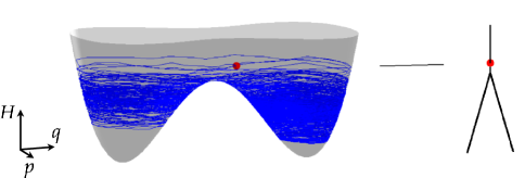
Figure 1. A single run of the SDE (3). The graph on the right-hand side is a reduction of the state space $\mathbb{R}^{2}$, according to the map $\Pi$; see the text for details.

Without the noise, the system is deterministic and preserves the Hamiltonian $H(q,p)=p^{2}/2+V(q)$, and solutions follow level sets of $H$. With noise, however, the Hamiltonian is not preserved, and the solutions follow a stochastic path that stays more or less close to a level curve, depending on the size of $\varepsilon$.

We will be interested in the limit $\varepsilon\to 0$; in this limit there is a separation of time scales, in which the solutions have a fast $H$-conserving drift, and follow level sets very closely over $O(\varepsilon)$ times, with velocity $O(1/\varepsilon)$; at $O(1)$ time scales the value of $H$ changes, and performs a biased Brownian motion, as was first proved by Freidlin and Wentzell [4]. We re-prove this result as an illustration of the method.

We write $X^{\varepsilon}=(Q^{\varepsilon},P^{\varepsilon})$ for the process in $\mathbb{R}^{2}$ described by the SDE (3) with a deterministic initial datum $x_{0}\in\mathbb{R}^{2}$, and we consider a sequence $X^{\varepsilon,i}$, $i=1,2,\dots$ of i.i.d. copies of this process. For this system Cattiaux and Léonard [1] prove the large-deviation principle (2) and the characterization (1).

The coarse-graining map $\Pi$ maps $\mathbb{R}^{2}$ to the graph $\Gamma$ consisting of equivalence classes of level sets of $H$, under the equivalence relation of belonging to the same connected component of the level sets of $H$. Below the saddle-point each level set has two connected components, thus leading to the two prongs in the graph $\Gamma$. For this system the method described above yields:

Theorem 1.

• $\hat{\rho}^{\varepsilon}\longrightarrow\hat{\rho}^{0}$ as $\varepsilon\to 0$ in $C([0,T];\mathcal{P}(\Gamma))$;

• $\liminf_{\varepsilon\to 0}I^{\varepsilon}(\rho^{\varepsilon})\geq\widehat{I}^{0}(\hat{\rho}^{0})$.

The liminf inequality in this theorem implies a type of convergence of solutions: the projected stochastic processes $Y^{\varepsilon}=\Pi(X^{\varepsilon})$ converge to biased diffusions on the graph $\Gamma$, and their behvaviour is fully characterized by the law $\mu\in\mathcal{P}(\Gamma)$ that uniquely satisfies $\widehat{I}^{0}(\mu)=0$. This equation can be shown to be equivalent to the diffusion-process description of [4], and to a weak-solution concept for a PDE.

References

- [1] P. Cattiaux and C. Léonard. Minimization of the Kullback information of diffusion processes. Ann. Inst. H. Poincaré Probab. Statist., 30(1):83–132, 1994.
- [2] M. H. Duong, M. A. Peletier, and U. Sharma. In preparation.
- [3] J. Feng and T. G. Kurtz. Large deviations for stochastic processes, volume 131 of Mathematical Surveys and Monographs. American Mathematical Society, 2006.
- [4] M. I. Freidlin and A. D. Wentzell. Random Perturbations of Hamiltonian Systems. American Mathematical Society, 1994.