Turbulent-laminar patterns in plane Poiseuille flow

Abstract

Turbulent-laminar banded patterns in plane Poiseuille flow are studied via direct numerical simulations in a tilted and translating computational domain using a parallel version of the pseudospectral code Channelflow. 3D visualizations via the streamwise vorticity of an instantaneous and a time-averaged pattern are presented, as well as 2D visualizations of the average velocity field and the turbulent kinetic energy. Simulations for $2300\geq Re_{b}\geq 700$ show the gradual development from uniform turbulence to a pattern with wavelength 20 half-gaps at $Re_{b}\approx 1900$, to a pattern with wavelength 40 at $Re_{b}\approx 1300$ and finally to laminar flow at $Re_{b}\approx 800$. These transitions are tracked quantitatively via diagnostics using the amplitude and phase of the Fourier transform and its probability distribution. The propagation velocity of the pattern is approximately that of the mean flux and is a decreasing function of Reynolds number. Examination of the time-averaged flow shows that a turbulent band is associated with two counter-rotating cells stacked in the cross-channel direction and that the turbulence is highly concentrated near the walls. Near the wall, the Reynolds stress force accelerates the fluid through a turbulent band while viscosity decelerates it; advection by the laminar profile acts in both directions. In the center, the Reynolds stress force decelerates the fluid through a turbulent band while advection by the laminar profile accelerates it. These characteristics are compared with those of turbulent-laminar banded patterns in plane Couette flow.

I Introduction: Phenomenon and Methods

The transition to turbulence is one of the least understood phenomena in fluid dynamics. Transitional regimes in wall-bounded shear flows display regular patterns of turbulent and laminar bands which are wide and oblique with respect to the streamwise direction. These patterns have been studied in counter-rotating Taylor-Couette flow Coles ; Andereck ; Hegseth89 ; Marques_PRE_09 ; Dong_PRE_09 ; Prigent_PRL ; Prigent_PhysD and in plane Couette flow Prigent_PRL ; Prigent_PhysD ; Barkley_PRL_05 ; Barkley_JFM_07 ; Tuckerman_PF_11 ; Manneville_PRE_11 ; Duguet_JFM_10 ; Duguet_PRL_13 ; Brethouwer .

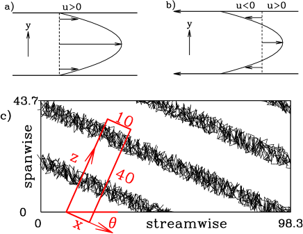
Figure 1: a) Standard (streamwise,cross-channel) view of plane Poiseuille flow in which $u_{\rm wall}\equiv u(y=\pm 1)=0$ and $u_{\rm bulk}\equiv\frac{1}{2}\int_{-1}^{1}u(y)dy=\frac{2}{3}$. b) Translating reference frame such that $u_{\rm wall}=-\frac{2}{3}$ and $u_{\rm bulk}=0$. c) Tilted reference frame in (streamwise, spanwise) view where $x$ is aligned with schematically drawn turbulent bands, at an angle of $\theta=24^{\circ}$ to the streamwise direction, and $z$ aligned with the pattern wave-vector. The tilted box has dimensions $L_{x}\times L_{z}=10\times 40$. In order to capture the same pattern, a box aligned with the streamwise and spanwise directions would be required to have dimensions $L_{\rm strm}\times L_{\rm span}=40/\sin(24^{\circ})\times 40/\cos(24^{\circ})=98.3\times 43.7$.

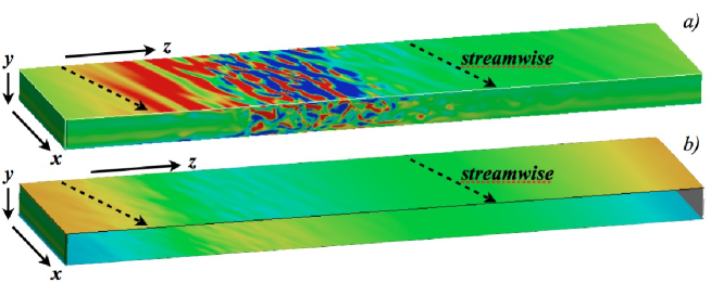
Figure 2: 3D visualization of the a) instantaneous and b) time-averaged $(\Delta T=8000)$ streamwise vorticity of a turbulent-laminar banded state at $Re=1100$ over the entire domain of size $L_{x}\times L_{y}\times L_{z}=10\times 2\times 40$. The bands are parallel to the $x$ direction, while the small-scale vortices are aligned in the streamwise direction (dashed arrows) which is oriented at an angle of 24^∘ to the $x$ direction. The maximum and minimum of the instantaneous streamwise vorticity is $\pm 6.2$ while that of the time-averaged vorticity is only $\pm 0.32$. Features of both are emphasized by choosing the color scale $[-0.5,0.5]$. The instantaneous vorticity, while strongest on the bounding plates, is present throughout the domain, as shown by the $(y,z)$ plane in front. This plane is omitted from the time-averaged vorticity to reveal contrasting views on the upper and lower plates; the antisymmetry in the vorticity results from the $y$-reflection symmetry of the average velocity.

Turbulent-laminar banded patterns have also been observed numerically and experimentally in plane Poiseuille (channel) flow by Tsukahara et al. Tsukahara_TSFP_05 ; Tsukahara_THMT_06 ; Tsukahara_ASCHT_07 ; Hashimoto_THMT_09 . Tsukahara et al. Tsukahara_THMT_06 presented detailed visualizations from numerical simualtions of the mean flow as well as the effect of turbulent bands on heat transport. Later experiments Hashimoto_THMT_09 compared the range of Reynolds numbers, wavelengths and angles of the turbulent bands obtained experimentally with the numerical results reported by Tsukahara et al. Tsukahara_ASCHT_07 . Brethouwer et al. Brethouwer simulated a turbulent-laminar pattern in Poiseuille flow as part of a larger study investigating the effects of damping by Coriolis, buoyancy and Lorentz forces on patterns in transitional flows. The goal of the present paper is to extend this work using methods previously employed to study turbulent-laminar banded patterns in plane Couette flow. In particular, we wish to determine if these patterns can be reproduced in the minimal geometry used in simulations of plane Couette flow Barkley_PRL_05 ; Barkley_JFM_07 ; Tuckerman_PF_11 , and to describe their evolution in time, their propagation velocity, and the balance of forces they entail.

Plane Poiseuille flow is generated by an imposed pressure gradient or an imposed bulk velocity between two parallel rigid plates. The length scale for nondimensionalization is half the distance between the plates. For a velocity scale, several choices are common, leading to several definitions of the Reynolds number: $Re_{c}$ uses the velocity at the center of the channel, $Re_{b}$ uses the bulk velocity, and $Re_{\tau}$ uses the wall shear velocity. One standard choice, and that made here, is to impose the bulk velocity and to scale the velocity by $3u_{\rm bulk}/2$, because this leads to $Re_{b}=Re_{c}$ for the laminar flow. Many of the references we cite use another factor, one Brethouwer or two Tsukahara_TSFP_05 ; Tsukahara_THMT_06 ; Tsukahara_ASCHT_07 ; Hashimoto_THMT_09 ; Kim , in place of the 3/2; when we cite Reynolds numbers from these references we have multiplied them by the appropriate conversion factor of 3/2 or 3/4. Unless mentioned otherwise, the Reynolds number $Re_{b}$ is denoted merely by $Re$.

The computational domain used in this study is tilted with respect to the bulk velocity, as illustrated in Fig. 1c, in order to efficiently capture similarly tilted laminar-turbulent patterns. As was done for plane Couette flow Barkley_PRL_05 ; Barkley_JFM_07 ; Tuckerman_PF_11 , the horizontal part of the domain is a narrow rectangle whose short direction (here, the $x$ axis, with $L_{x}=10$) is parallel to the expected direction of the bands, at an angle of 24^∘ from the streamwise direction. The long direction (here, the $z$ axis, with $L_{z}=40$) is parallel to the expected wave-vector of the bands. Thus:

$$\mathbf{\hat{e}}_{\rm strm} = \cos 24^{\circ}\>\mathbf{\hat{e}}_{x}+\sin 24^{\circ}\>\mathbf{\hat{e}}_{z},$$ (1a)

$$\mathbf{\hat{e}}_{\rm span} =- \sin 24^{\circ}\>\mathbf{\hat{e}}_{x}+\cos 24^{\circ}\>\mathbf{\hat{e}}_{z}$$ (1b)

The reason for choosing $24^{\circ}$ in plane Couette flow was that this angle is in the range $[24^{\circ},37^{\circ}]$ observed experimentally in very large-scale experiments Prigent_PRL ; Prigent_PhysD (770 by 340 half-gaps in the streamwise and spanwise directions, respectively), in which the flow was free to choose its own angle; this range of angles is also observed in simulations by Duguet et al. Duguet_JFM_10 in a domain of similar size. This is also the case for plane Poiseuille flow. Tsukahara et al. Tsukahara_TSFP_05 ; Tsukahara_THMT_06 first produced turbulent-laminar patterns in a domain with dimensions of 51.2 by 22.5 in the streamwise and spanwise directions, leading by construction to $\theta=\tan^{-1}(22.5/51.2)=23.7^{\circ}$. The domain used by Brethouwer et al. Brethouwer is very similar (55 by 25) and hence leads to a similar angle of $24.4^{\circ}$. Later simulations Tsukahara_ASCHT_07 in a domain of size 328 by 128 (in which the flow was relatively free to choose its own angle) produced patterns with angles in the range $[20^{\circ},25^{\circ}]$ while the experiments of Tsukahara et al. Hashimoto_THMT_09 showed angles in the range $[20^{\circ},30^{\circ}]$. Our narrow tilted domain enforces an angle of $24^{\circ}$; only patterns with this angle can be simulated.

The tilted $x$ and $z$ directions are taken to be periodic and $y$ is the usual cross-channel direction. The streamwise, cross-channel and spanwise velocities continue to be denoted by ${\bf u}=(u,v,w)$ (even though $x,y,z$ do not correspond to these directions). In order to follow the patterns as they advect with the bulk flow, computations are performed in a moving reference frame whose velocity matches the constant (nondimensionalized) streamwise bulk velocity of 2/3. In this reference frame the walls move at $-2/3$ in the streamwise direction, and the imposed mean velocity is zero in both the span and streamwise directions. All velocities in this study are reported with respect to the moving reference frame (except those involved in the definition of Reynolds numbers, which are relative to fixed walls). The domain size is $L_{x}\times L_{y}\times L_{z}=10\times 2\times 40$. The choice of $L_{z}$ was guided by considerations similar to those for the angle, i.e. results from experiments and simulations in plane Couette flow and plane Poiseuille flow. All of the references cited previously  Brethouwer ; Tsukahara_TSFP_05 ; Tsukahara_THMT_06 ; Tsukahara_ASCHT_07 ; Hashimoto_THMT_09 reported patterns with wavelengths in the range $[20,30]$. In our domain, only patterns whose wavelength is a divisor of $L_{z}$ can be simulated, i.e. 40, 20, 10, etc. The choice $L_{x}=10$ is dictated by the requirement that the box be large enough to sustain turbulence, more specifically that the spanwise dimension $L_{x}\sin\theta$ be wide enough to accomodate a pair of streamwise vortices Jimenez_91 ; Hamilton ; Waleffe_03 ; Barkley_PRL_05 ; Barkley_JFM_07 ; Tuckerman_PF_11 .

Streamwise vortices are indeed a prominent feature of turbulent regions, as shown in the visualization in Fig. 2a of a computed turbulent-laminar pattern. The streamwise vorticity is particularly appropriate for representing turbulence in plane Poiseuille flow since it is zero for laminar flow and is not zero at the plates, near which the turbulence is most intense. The instantaneous vorticity, Fig. 2a, is localized in one region of the domain and is aligned in the streamwise direction. Figure 2b shows the streamwise vorticity averaged over $\Delta T=8000$ time units. The time-averaged vorticity is much weaker than the instantaneous vorticity, and is antisymmetric under reflection in $y$, showing that the corresponding velocity is reflection-symmetric in $y$.

Figure 3: Spatio-temporal plots from simulations in domain of size $L_{x}\times L_{y}\times L_{z}=10\times 2\times 40$ in which the $z$ direction is oriented along the pattern wave-vector. Spanwise velocity timeseries $w(z_{j},t)$ are shown for points along the line $x=0$, $y=0.8$ at 32 equally spaced values $z_{j}=jL_{z}/32$ for $2300\geq Re\geq 800$. Uniform turbulence can be seen for $Re=2300$, traces of laminar patches for $2200\geq Re\geq 2000$, increasingly well-defined left-going bands of wavelength 20 for $1900\geq Re\geq 1400$, a change in wavelength and direction for $Re=1300$, 1200, and an increasingly weak and fragile right-going pattern of wavelength 40 for $1100\geq Re\geq 800$.

The simulations were performed with a parallelized version of the pseudospectral C++-code Channelflow channelflow , which employs Fourier-Chebyshev spatial discretization, fourth-order semi-implicit backwards-differentiation time stepping, and an influence matrix method with Chebyshev tau correction on the primitive-variables formulation of the Navier-Stokes equations (Orszag, ; Kleiser, ; Kim, ; Peyret, ). The code uses FFTW Frigo2005 for Fourier transforms and MPI for parallelization. We use $N_{x}\>\times\>(N_{y}+1)\>\times\>N_{z}=128\;\times\;65\;\times\;512=4.2\times 10^{6}$ points or modes to represent the domain of size $L_{x}\times L_{y}\times L_{z}=10\times 2\times 40$, with a spacing of $\Delta x=\Delta z=0.08$ and $\Delta y$ ranging from $\Delta y_{\rm wall}=1-\cos(\pi/64)=0.001$ to $\Delta y_{\rm mid}=\cos(31\pi/64)=0.05$. For the highest Reynolds number we simulate, $Re=2300$, the ratio between the viscous wall unit and the half-gap is 0.009, so $\Delta x^{+}=\Delta z^{+}=0.08/0.009=9$, $\Delta y_{\rm wall}^{+}=0.001/0.009=0.11$ and $\Delta y_{\rm mid}^{+}=0.05/0.009=5.6$. For plane Poiseuille flow, it is crucial to have sufficient resolution in the cross-channel direction near the walls, where the turbulence is concentrated. The resolution used here is similar to that used in the simulations by Kim et al. Kim ($Re=4200$; $Re_{\tau}=180$) and Jiménez & Moin Jimenez_91 ; although these authors used $N_{y}=128$, they studied Reynolds that were about twice the highest Reynolds number investigated here and stated that using $N_{y}=64$ produced similar results Kim . In terms of wall units, our resolution is the same or finer than that used in these studies. Our resolution is also close to that used by Tsukahara et al. Tsukahara_TSFP_05 ; Tsukahara_THMT_06 for $Re=1732$ ($Re_{\tau}=80$) and $Re=1327$ ($Re_{\tau}=64$) and higher than that of Brethouwer et al. Brethouwer , who used $\Delta x^{+}=15$, $\Delta z^{+}=6.7$ and $N_{y}=32$ for a case with $Re=700$ ($Re_{\tau}=69$). The timestep varied from $\Delta t=0.03$ for $Re=900$ to $\Delta t=0.015$ for $Re=2300$. Simulations run on the IBM x3750 of the IDRIS supercomputer center using 32 processes typically took about 16 wall clock hours to simulate 10 000 advective time units.

II Reynolds-number scan

Figure 3 shows spatio-temporal diagrams of the spanwise velocity. For $Re\leq 2000$, each simulation is a continuation of the corresponding part of a long simulation in which the Reynolds number is decreased in discrete decrements of 100, which will be presented in Fig. 6 and which itself is initialized with random noise. The simulations with $Re>2000$ were all initialized with the final state of the $Re=2000$ run. The timeseries show $w(z_{j},t)$ at $x=0$, $y=0.8$ (near the upper plate), for 32 values $z_{j}$ separated by intervals of $\Delta z=L_{z}/32$ for Reynolds numbers varying from 2300 down to 800. Dark patches indicate rapid large-amplitude oscillations in the spanwise velocity, i.e. turbulent regions. The surrounding lighter patches are composed of straight lines, indicating locations at which the spanwise velocity remains constant or nearly so, i.e. quasi-laminar regions.

For the highest Reynolds number, $Re=2300$, the entire interval $0\leq z\leq L_{z}$ is dark, indicating turbulence which is statistically uniform over the domain. As $Re$ is lowered to 2100, quiescent patches appear which move towards the left (opposite to $(u_{\rm mean}-u_{\rm wall})$). Timeseries for $1900\geq Re\geq 1400$ show two clearly delineated turbulent bands with a fairly well-defined wavelength and velocity. From $Re=1300$ to $Re=1200$, there is a transition from two to one turbulent band. New turbulent patches repeatedly branch off from existing ones; these are more persistent and long-lasting for $Re=1300$ than for 1200. The velocity of the pattern decreases. For $Re=1100$, the pattern comprises a single band and is almost stationary; the band begins to disappear at $T=8700$, becoming completely laminar by $T=9000$. For $Re=1000$ and 900, a single right-going band is present, which, for $Re=900$ disappears at $T=9700$. For $Re=800$, the band disappears earlier, at around $T=2200$.

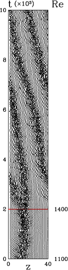
a) b)

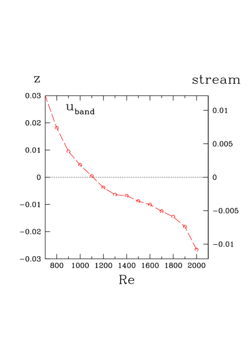
Figure 4: a) Simulation in domain of size $L_{x}\times L_{y}\times L_{z}=10\times 2\times 40$, with conventions as in Fig. 3. When $Re$ is increased from 1100 to 1400, the pattern with one turbulent band is quickly replaced by a left-moving pattern with two bands. Propagation speed of turbulent bands with respect to the mean flow. At $Re\approx 1100$, the bands move at approximately the same speed as the mean flow. For $Re\lesssim 1100$, the bands move more quickly than the mean flow, while for $Re\gtrsim 1100$, they move more slowly. The scale on the left (right) indicates the velocity in the $z$ (streamwise) direction; the two scales are related by the trigonometric factor $\sin 24^{\circ}$.

For plane Couette flow, a qualitative distinction can be made between patterns at higher $Re$, in which the turbulent and quasi-laminar regions each occupy approximately half of the domain, and patterns at lower $Re$, in which the turbulent band occupies a smaller fraction of the domain. The averaged high-$Re$ patterns were shown Barkley_JFM_07 to have a trigonometric dependence on $z$. In contrast, the bands at lower $Re$ were shown to be isolated states, in that they retain their size when placed in a wider domain Barkley_PRL_05 and are surrounded by truly laminar regions. A comparison of the states at $Re\geq 1400$ with those at $Re\leq 1100$ shows that this distinction seems also to apply to plane Poiseuille flow. For $Re\geq 1400$, the turbulent bands occupy about half the width of the domain, with the other half consisting of slightly chaotic flow, as shown by the small-scale oscillations in $w(z_{j},t)$. For $Re\leq 1100$, the single turbulent band occupies much less than the width of the domain and the flow reverts to laminar quite close to the boundaries of the band, as shown by the straight lines $w(z_{j},t)$ for $z_{j}$ within a few multiples of $L_{z}/32$.

The branching events at $Re=1300$ and $Re=1200$ indicate bistability between a pattern with wavelength 40 and wavelength 20; a domain with a larger or different $L_{z}$ would almost surely display patterns with intermediate wavelengths and bistability at a different value of $Re$. There is also clearly an important random component in the fact that relaminarisation occurs at $Re=1100$ but not at $Re=1000$. Simulations with different initial conditions would almost surely lead to relaminarisation at different times; the properties of these events must be studied statistically, as has been done for pipe flow Peixinho_JFM_07 ; Avila_Science and for Couette flow Shi . Although we have not checked systematically for hysteresis, when we increased the Reynolds number from 1100 to 1400, the initial single quasi-stationary band evolved quickly to a left-moving pattern with two bands; see figure 4a).

Figure 4b) shows the propagation velocity as a function of $Re$. Propagation in the $z$ direction is to be expected, since there is a substantial overlap between the $z$ direction and the streamwise direction. The fact that the speeds are so small demonstrates that the turbulent bands move essentially at the speed of the mean flow, as was noted by Tsukahara et al. Tsukahara_THMT_06 ; Hashimoto_THMT_09 . As was seen in Fig. 3, $Re\approx 1100$ separates propagation to the left (slower than the mean flow) and to the right (faster than the mean flow). It is because the pattern at $Re=1100$ is approximately stationary in the frame of the mean flow that this Reynolds number was chosen to display the time-averaged flow shown in Fig. 2. Although the number of bands is quantized, their velocity is not; moreover the velocity varies smoothly through the change in the number of bands at $Re=1100$. Therefore it seems likely that that the velocity presented in Fig. 4b) is independent of the domain. Propagation velocities are in general quite sensitive to resolution; previous simulations with less resolution in $y$ showed the propagation velocity to change sign at $Re=1400$ instead of $Re=1100$. We have verified that the velocity does not change appreciably with higher resolution.

An overall view of the evolution of the pattern can be seen in the Reynolds-number scan of Fig. 6. This figure describes a simulation initialized at $Re=2000$ with a random initial condition and in which the Reynolds number is lowered in discrete steps of 100, remaining at each $Re$ for a time of length $\Delta T=2000$. (The simulations of length $\Delta T=10\,000$ in Fig. 3 are continuations for another $\Delta T=8000$ of each of the sections of Figure 6). Figure 6a shows streamwise velocity profiles $u(y)$ at intervals of $\Delta T=2000$ at a fixed value of $x$ and $z$; these are flat or parabolic, depending on whether the corresponding flow or region is turbulent or laminar. Figure 6b, like Fig. 3, shows timeseries of the spanwise velocity $w(z_{j},t)$ at 32 equally spaced points in $z$.

The evolution from the random initial condition at $Re=2000$ leads rapidly to turbulence which is uniform (without bands). As $Re$ is lowered past $Re\approx 1800$, two quiescent patches appear (though the long time series of Fig. 3 show that a muted version of this pattern already appears for higher $Re$, given sufficient time). Several transitions are clearly visible: from two turbulent bands to one at $Re=1200$, from leftwards to rightwards motion at $Re=1100$, and from one turbulent band to none at $Re=700$.

Figures 6c,d show that these tendencies can be measured quantitatively via the modulus $|\hat{w}_{m}(t)|$ and the phase $\hat{z}_{m}(t)$ of the discrete Fourier transform in $z$:

$$w(z_{j},t)=\sum_{m}\hat{w}_{m}(t)e^{imz_{j}\frac{2\pi}{L_{z}}}=\sum_{m}|\hat{w}_{m}(t)|e^{im(z-\hat{z}_{m}(t))\frac{2\pi}{L_{z}}}\vspace*{-0.2cm}$$ (2)

averaged over appropriate time intervals:

$$\langle|\hat{w}_{m}(t)|\rangle {}_{1000}\equiv \frac{1}{1000}\int_{t^{\prime}=0}^{1000}dt^{\prime}\;|\hat{w}_{m}(t+t^{\prime})|$$ (3a)

$$\langle\hat{z}_{m}(t)\rangle_{100} \equiv \frac{1}{100}\int_{t^{\prime}=0}^{100}dt^{\prime}\;\hat{z}_{m}(t+t^{\prime})$$ (3b)

In Fig. 6c, $\langle|\hat{w}_{2}(t)|\rangle_{1000}$ rises from a low value when $Re$ is decreased below 1900, and is then overtaken by $\langle|\hat{w}_{1}(t)|\rangle_{1000}$ at $Re=1200$, when one of the turbulent bands disappears. Although the pattern for $1200\geq Re\geq 800$ has wavelength $\lambda=40$, it also contains higher harmonics and so $\hat{w}_{2}$ remains non-negligible.

Figure 6d shows the averaged phases $\langle\hat{z}_{m}(t)\rangle_{100}$. When the modulus is small, the phase loses significance, so phases are shown only when the modulus exceeds a heuristically determined threshold, 0.24 for $m=1$ and 0.4 for $m=2$. The phases $\langle\hat{z}_{2}(t)\rangle_{100}$ and $\langle\hat{z}_{2}(t)\rangle_{100}+L_{z}/2$ track the centers of the two turbulent bands seen in Fig. 6b for $1800\geq Re>1200$, while $\langle\hat{z}_{1}(t)\rangle_{100}$ tracks the center of the single turbulent band for $1200\geq Re\geq 800$.

The instantaneous values of $a(t)\equiv|\hat{w}_{m}(t)|$ collected for each Reynolds number during the time that the flow is partly or entirely turbulent (see Fig. 3) can also be used to construct probability distribution functions. Because $|\hat{w}_{m}(t)|$ is a modulus, the range $a_{j-1}<|\hat{w}_{m}(t)|\leq a_{j}$ corresponds to an annulus in the two-dimensional Cartesian space of $(\hat{w}_{m}^{r},\hat{w}_{m}^{i})$ of area

$$\pi(a_{j}^{2}-a_{j-1}^{2})=2\pi\frac{(a_{j}+a_{j-1})}{2}(a_{j}-a_{j-1})$$ (4)

The bin boundaries $a_{j}$ can be chosen to correspond to annuli of equal size by taking

$$a_{j} \equiv \sqrt{\frac{j}{N_{\rm bin}}}\max_{t}|\hat{w}_{m}(t)|$$ (5a)

$$p_{j} \propto |\{t:a_{j-1}<|\hat{w}_{m}(t)|\leq a_{j}\}|$$ (5b)

where $|\{\}|$ denotes the number of elements of a set. Another possibility is to choose bin boundaries $a_{j}$ which are equally spaced and to correct for the difference in annular areas (4) by dividing $p_{j}$ by $(a_{j}+a_{j-1})/2$. A third possibility is to choose bin boundaries such that each bin contains the same number of values, and to divide $p_{j}$ by $(a_{j}-a_{j-1})(a_{j}+a_{j-1})/2$. All three procedures lead to similar probability distribution functions.

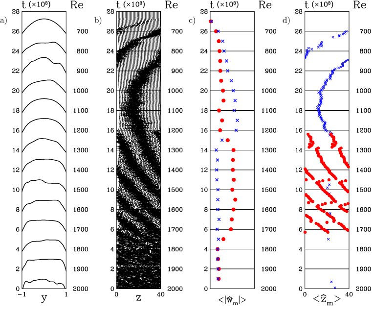
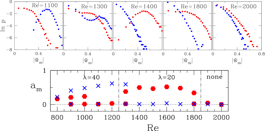
Figure 5: Simulations in domain of size $L_{x}\times L_{y}\times L_{z}=10\times 2\times 40$ The Reynolds number is decreased from 2000 to 700 in discrete steps at time intervals of $\Delta T=2000$, as indicated along the axes on the right.
a) Instantaneous representative streamwise velocity profiles $u(y)$ along the line $x=z=0$ at intervals of $\Delta T=2000$.
b) Spanwise velocity timeseries $w(z_{j},t)$ along the line $x=0$, $y=0.8$ at 32 equally spaced values $z_{j}=jL_{z}/32$.
c) Temporal average $\langle|\hat{w}_{m}(t)|\rangle_{1000}$ (arbitrary units) of the modulus of the $z$-Fourier transform $\hat{w}_{m}$ of the spanwise velocity.
d) Temporal average $\langle\hat{z}_{m}(t)\rangle_{100}$ of the phase of $\hat{w}_{m}$ at times for which $\langle|\hat{w}_{m}(t)|\rangle_{100}$ is sufficiently large.
For c),d), the red disks indicate $m=2$ ($\lambda=20$), while the blue crosses indicate $m=1$ ($\lambda=40$).

Figure 6: Above: probability distributions of the moduli of the Fourier components $|\hat{w}_{m}(t)|$ for $m=1$ and $m=2$ for representative values of the Reynolds number. Below: maxima of the PDFS as a function of Reynolds number showing changes in regime at $Re\approx 1900$ and $Re\approx 1300$. The red disks indicate $m=2$ ($\lambda=20$), while the blue crosses indicate $m=1$ ($\lambda=40$). The maximum of both PDFS is located at zero for $Re\geq 1900$. For $1900>Re\geq 1300$, the $m=2$ PDF has a maximum away from zero, indicating a pattern of this wavenumber. For $1300\geq Re\geq 800$, the $m=1$ PDF has a maximum away from zero, indicating a pattern of this wavenumber.

Figure 6 displays probability distribution functions for $m=1$ and $m=2$ for representative Reynolds number values. In the absence of a pattern, in particular for uniform turbulence, the maximum (most probable value) for $|\hat{w}_{m}(t)|$ is zero, while for patterned flows, the maximum is non-zero. The PDFs yield thresholds:
$\bullet$ $Re\approx 1900$, separating uniform turbulence and a pattern with $m=2$, i.e. $\lambda=20$
$\bullet$ $Re\approx 1300$, separating patterns with $m=2$ and $m=1$, i.e. $\lambda=20$ and $\lambda=40$
$\bullet$ $Re\approx 800$, separating a pattern with $m=1$ from laminar Poiseuille flow.

III Mean flow and force balance

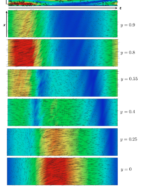
Figure 7: Time-averaged deviation from laminar flow at $Re=1100$ on a typical $(z,y)$ plane (top) and on $(x,z)$ planes at various values of $y$. The $(z,y)$ plot has been stretched by a factor of 3 in the $y$ direction for visibility. Flow for $y<0$ resembles that for $y>0$. Arrows indicate the direction of the velocities while colors indicate its magnitude. Scale [0,0.2].

Figure 7 presents views on various planes of the deviation of the time-averaged flow from the laminar velocity. The Reynolds number is 1100, as in Fig. 2. The flow varies a great deal with $y$ and $z$, but depends little on $x$, as predicted for the tilted domain. In order to gain more insight into this flow, we therefore form a 2D field by averaging over $L_{x}$ as well as $\Delta T=8000$:

$$\langle{\bf u}\rangle(y,z)\equiv\int_{t=0}^{8000}dt\int_{x=0}^{L_{x}}{\bf u}(x,y,z,t)$$ (6)

where $\langle\rangle$ has been redefined from (3). Fig. 8 presents various aspects of $\langle{\bf u}\rangle$. This figure agrees extremely well with Fig. 3 of Tsukahara et al. Tsukahara_THMT_06 , which shows similar quantities for a patterned flow at $Re=1327$ averaged over time and $L_{x}$. Tsukahara et al. Tsukahara_THMT_06 do not show the spanwise velocity, and include a number of other quantities such as the shear stress and Reynolds shear stress not shown here. The field is reflection-symmetric in $y$. (Reflection in $y$ changes the sign of the cross-channel velocity, as it does for the streamwise vorticity shown in Fig. 2b.)

Figure 8a shows the streamwise velocity. Unlike the other parts of Fig. 8, this subfigure includes the laminar flow. The waviness corresponds to the alternation of parabolic and plug profiles which occur in laminar and turbulent regions, respectively. The cross-channel velocity (Fig. 8b) still shows small-scale features despite the averaging over $L_{x}$ and $\Delta T=8000$. The spanwise velocity (Fig. 8c) shows distinctive chevron features. Figure 8d depicts the streamfunction associated with the deviation of the mean velocity from the laminar flow in the $(y,z)$ plane. Two wide counter-rotating cells are stacked in the gap. This is also the form of the mean flow observed experimentally in the presence of a turbulent spot by Lemoult et al. Lemoult_EPJE . The direction of rotation of these cells is such as to slow the streamwise flow in the middle of the channel and accelerate it near the walls, in effect transforming a parabolic profile to the slug profile.

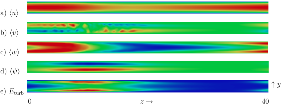
Figure 8: Mean flow in the $(y,z)$ plane from simulation at $Re=1100$ averaged over $L_{x}$ and over time of $\Delta T=8000$.
a) Streamwise velocity $\langle u\rangle$ including laminar profile: the undulations correspond to profiles which are slug-like (turbulent regions) or parabolic (laminar regions) in Fig. 6a. Scale $[-0.67,0.33]$.
b) Cross-channel velocity $\langle v\rangle$: small-scale structures are still visible despite averaging. Scale $[-0.003,0.003]$.
c) Spanwise velocity $\langle w\rangle$ with characteristic chevrons. Scale $[-0.05,0.05]$.
d) Streamfunction $\langle\psi\rangle$ shows two superposed layers of cellular flow in the $(y,z)$ plane. The laminar velocity has been subtracted.
e) Turbulent kinetic energy $E_{\rm turb}$: the red regions show a strong concentration near the bounding plates. Scale $[0,0.012]$.

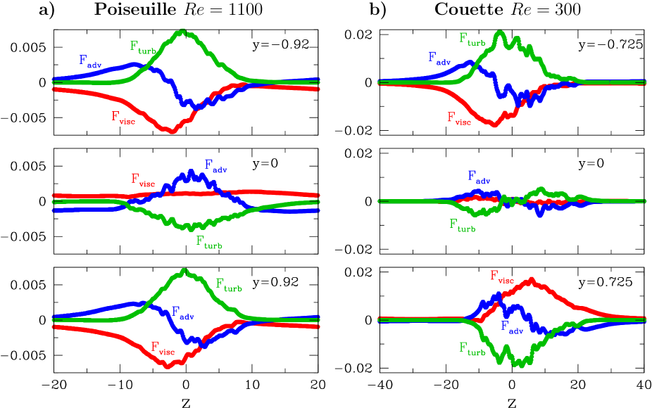
Figure 9: Streamwise Reynolds stress (green, (9a)), advective (blue, (9b)) and viscous (red, (9c)) forces as a function of $z$ at three $y$ locations for the mean flow associated with turbulent-laminar (a) Poiseuille flow at $Re=1100$ and (b) Couette flow at $Re=300$. Near the lower wall ($y<0$), for both flows, the Reynolds stress force accelerates the fluid through the turbulent band while the viscous force decelerates it; advection by the basic laminar flow changes sign in the middle of the band. In the center ($y=0$), for Poiseuille flow, advection accelerates the fluid while the Reynolds stress force decelerates it; for Couette flow, this situation is reversed over half the turbulent region. Near the upper wall ($y>0$), the force balance for Poiseuille flow is identical to that near the lower wall; for Couette flow the balance near the upper and lower walls are related by centro-symmetry.

Figure 8e presents the turbulent kinetic energy defined by

$$E_{\rm turb}\equiv\frac{1}{2}\langle\tilde{{\bf u}}\cdot\tilde{{\bf u}}\rangle,\qquad\tilde{{\bf u}}\equiv{\bf u}-\langle{\bf u}\rangle$$ (7)

which is concentrated very near the boundaries, where the shear of the laminar profile is greatest. The counter-rotating cells (d) are centered at the same value of $z$ as the turbulent kinetic energy (e), but the maximum deviation in the streamwise velocity (a) is located to the right of this location. A shift between these quantities was previously noted by Tsukahara et al. Tsukahara_THMT_06 as well as in the case of plane Couette flow Prigent_PRL ; Prigent_PhysD ; Barkley_JFM_07 ; Tuckerman_PF_11 .

We can compare the appearance of these mean quantities with the analogous ones in Fig. 5 of Barkley and Tuckerman Barkley_JFM_07 for plane Couette flow. As is the case for plane Couette flow, variation in $z$ is much slower than variation in $y$, For plane Couette flow, the turbulent kinetic energy occupies most of the interior of the gap and the $(y,z)$ flow consists of a single large rotating cell. An obvious difference between the two flows is symmetry: plane Poiseuille flow is reflection-symmetric in $y$, while plane Couette flow is centro-symmetric in $(y,z)$. That is, variables $u$ and $w$ obey

$$F(-y,z)= F(y,z)\qquad$$ Poiseuille (8a)

$$F(-y,z)= -F(y,-z)\qquad$$ Couette (8b)

For other quantities, e.g. $v$ or $\psi$, the change in sign is opposite to that in (8a) and (8b). One of the striking properties of turbulent-laminar banded patterns is that their mean flow inherits the symmetries of the laminar flow.

Figure 9a shows the main forces acting in the streamwise direction on the mean flow:

$$F_{\rm turb} \equiv -\langle(\tilde{{\bf u}}\cdot\nabla)\tilde{{\bf u}}\rangle$$ (9a)

$$F_{\rm adv} \equiv -\left({\bf u}_{\rm lam}\cdot\nabla\right)\langle u-u_{\rm lam}\rangle$$ (9b)

$$F_{\rm visc} \equiv \frac{1}{Re}\nabla^{2}\langle u-u_{\rm lam}\rangle$$ (9c)

We omit the larger forces governing laminar Poiseuille flow:

$$\nabla p_{\rm lam}=\frac{1}{Re}\nabla^{2}{\bf u}_{\rm lam}=-\frac{2}{Re}{\bf e}_{\rm strm}$$ (10)

as well as the smaller pressure gradient associated with $\langle{\bf u}-{\bf u}_{\rm lam}\rangle$ and the nonlinear interaction of $\langle{\bf u}-{\bf u}_{\rm lam}\rangle$ with itself. The three forces are plotted as a function of $z$ for values of $y$ near the two walls and at the center of the channel. To interpret Fig. 9, it is helpful to recall that while $z$ is not the streamwise direction, it has a component in this direction; see Fig. 1c. Thus a streamwise force which is positive (negative) accelerates (decelerates) the fluid towards the right (left) in the $z$ direction.

Figure 9b shows the balance of forces for an analogous state in plane Couette flow. We have chosen $Re=300$ because at this Reynolds number, the turbulence in plane Couette flow is localized Barkley_PRL_05 , as is the case for plane Poiseuille flow at $Re=1100$. See section IV for a discussion on converting between scales in Couette and Poiseuille flows. The domain of length $L_{z}=80$ is chosen to be twice that of the domain we used for Poiseuille flow. For each flow, the origin in $z$ has been translated so that the turbulent region is at the center of the graph. The nonzero $y$ positions for which the forces are plotted are those for which the forces are maximal. The different symmetries of the two flows, i.e. $y$-reflection for Poiseuille and centro-symmetry in $(y,z)$ for Couette flow, are clearly visible in Fig. 9.

The upper panels show the forces for $y<0$, where the shear of both basic flows is positive. The resemblance between the force balance for the two flows is remarkable. For both flows, $F_{\rm turb}$ is large and positive in the turbulent region, accelerating the fluid towards the right, and is counterbalanced primarily by $F_{\rm visc}$. The advective force $F_{\rm adv}$ is comparable but smaller in magnitude; it acts with $F_{\rm turb}$ in the left portion of the turbulent region and against $F_{\rm turb}$ in the right portion. At the center ($y=0$), the curvature $\partial_{y}^{2}u$ and hence $F_{\rm visc}$ is small for Poiseuille flow and negligible for Couette flow, For Poiseuille flow, $F_{\rm adv}$ accelerates the fluid in the turbulent region, while $F_{\rm turb}$ decelerates it. For Couette flow, this holds over half the turbulent region, while the reverse is true over the other half, as required by (8b). For $y>0$, the flow and forces for Poiseuille flow are the same as for $y<0$, while for Couette flow the flow and forces are reversed from those at $y<0$.

IV Discussion

We conclude with some further comparisons between turbulent-laminar bands in Poiseuille and Couette flow. It has been proposed by Waleffe Waleffe_03 that plane Poiseuille flow can be viewed as two superposed plane Couette flows. This is consistent with the two cells and two turbulent regions seen in Fig. 8d,e. The similarity in the balance of forces shown in figure 9 also strongly supports the idea that turbulent-laminar patterns are maintained by the same physical mechanisms in Poiseuille and Couette flow.

With this in mind, we compare the wavelengths and Reynolds numbers of turbulent-laminar banded patterns in Poiseuille and Couette flow. In our domain, the wavelength of the patterns in plane Poiseuille flow is 20 at higher $Re$ and becomes 40 for lower $Re$. Turbulent-laminar patterns in plane Couette flow have higher wavelengths Prigent_PRL ; Prigent_PhysD ; Barkley_PRL_05 ; Barkley_JFM_07 ; Tuckerman_PF_11 : 40 for higher $Re$ and 60 for lower $Re$. The idea of considering Poiseuille flow as two superposed Couette flows suggests that Poiseuille flow should be scaled by the quarter-gap rather than the half-gap. This would make the pattern wavelength of 40 (quarter-gaps) of plane Poiseuille flow at higher $Re$ consistent with the wavelength of 40 (half-gaps) observed for plane and Taylor-Couette flow. It was already observed Prigent_PhysD ; Barkley_JFM_07 that a unified Reynolds number $Re_{s}$ based on the square of the $y$-averaged shear of the laminar flow and the quarter gap for plane Poiseuille flow could be defined to yield $Re_{s}=Re_{c}/4\approx Re/4.6$. For plane Couette flow, using the constant shear and the half-gap, $Re_{s}$ is the usual Reynolds number. The range of existence $800\leq Re\leq 1900$ for turbulent-laminar patterns in plane Poiseuille flow becomes $174\leq Re_{s}\leq 413$, which is of the same order as the range of existence $[300,420]$ for turbulent-laminar patterns in plane Couette flow. We note that the Reynolds-number range over which patterned turbulence is obtained by Tsukahara et al. is $Re_{b}\in[1125,2250]$, i.e. $Re_{s}\in[245,490]$ in numerical simulations Tsukahara_ASCHT_07 and $Re_{b}\in[1275,1500]$, i.e. $Re_{s}\in[277,326]$ in experiments Hashimoto_THMT_09 . It would be unlikely to obtain more precise agreement since the analogy between Poiseuille and Couette flow is inexact in a number of ways. For example, the turbulent near-wall regions of plane Poiseuille flow occupy considerably less than a quarter-gap. Second, in seeking a single measure of the shear in plane Poiseuille flow, it is not clear that a simple average is the best candidate.

An important consequence of the differences in symmetry is that the moderate-time averages of the turbulent-laminar patterns in Couette flow are stationary while those of Poiseuille flow have a well-defined velocity, which we have shown in Fig. 4b).

It is almost surely possible to produce patterns at angles quite different from $24^{\circ}$. In large-scale experiments in plane Couette flow Prigent_PRL ; Prigent_PhysD patterns were observed whose angles ranged between $24^{\circ}$ and $37^{\circ}$; simulations in narrow tilted domains with imposed angles ranging from $15^{\circ}$ and $66^{\circ}$ all produced patterns Barkley_PRL_05 ; Barkley_JFM_07 ; Tuckerman_PF_11 . The simulated patterns whose angles are far outside the range $[24^{\circ},37^{\circ}]$ would presumably be unstable when placed in a less constrained geometry. Although the narrow tilted geometry – the analogue of the minimal flow unit Jimenez_91 ; Hamilton for maintaining shear-flow turbulence – can be used to study some of the characteristics of turbulent-laminar patterns, studies in a less constrained geometry are necessary for understanding their genesis and fate. The spreading of turbulent spots and fronts have been widely studied for plane Poiseuille flow, e.g. experimentally by Lemoult et al. Lemoult_EPJE ; Lemoult_JFM_13 and numerically by Aida et al. Aida_TSFP_11 and as well as numerically by Duguet et al. Duguet_PRE_11 for plane Couette flow.

Future work will focus on the mechanism maintaining turbulent-laminar patterns and on the branching events that accompany the change in wavelength and in speed.

- (1) D. Coles, Transition in circular Couette flow, J. Fluid Mech. 21, 385 (1965).
- (2) C. D. Andereck, S. S. Liu, and H. L. Swinney, Flow regimes in a circular Couette system with independently rotating cylinders, J. Fluid Mech. 164, 155 (1986).
- (3) J. J. Hegseth, C. D. Andereck, F. Hayot, and Y. Pomeau, Spiral turbulence and phase dynamics, Phys. Rev. Lett. 62, 257 (1989).
- (4) A. Meseguer, F. Mellibovsky, M. Avila, and F. Marques, Instability mechanisms and transition scenarios of spiral turbulence in Taylor-Couette flow, Phys. Rev. E 80, 046315 (2009).
- (5) S. Dong, Evidence for internal structures of spiral turbulence, Phys. Rev. E 80, 067301 (2009).
- (6) A. Prigent, G. Grégoire, H. Chaté, O. Dauchot, and W. van Saarloos, Large-scale finite-wavelength modulation within turbulent shear flows, Phys. Rev. Lett. 89, 014501 (2002).
- (7) A. Prigent, G. Grégoire, H. Chaté, and O. Dauchot, Long-wavelength modulation of turbulent shear flows, Physica D 174, 100 (2003).
- (8) D. Barkley and L. S. Tuckerman, Computational study of turbulent laminar patterns in Couette flow, Phys. Rev. Lett. 94, 014502 (2005).
- (9) D. Barkley and L. S. Tuckerman, Mean flow of turbulent-laminar patterns in plane Couette flow, J. Fluid Mech. 576, 109 (2007).
- (10) L. Tuckerman and D. Barkley, Patterns and dynamics in transitional plane Couette flow, Phys. Fluids 23, 041301 (2011).
- (11) J. Philip and P. Manneville, From temporal to spatiotemporal dynamics in transitional plane Couette flow, Phys. Rev. E 83, 036308 (2011).
- (12) Y. Duguet, P. Schlatter, and D. S. Henningson, Formation of turbulent patterns near the onset of transition in plane Couette flow, J. Fluid Mech. 650, 119 (2010).
- (13) Y. Duguet and P. Schlatter, Oblique laminar-turbulent interfaces in plane shear flows, Phys. Rev. Lett. 110, 034502 (2013).
- (14) G. Brethouwer, Y. Duguet, and P. Schlatter, Turbulent-laminar coexistence in wall flows with Coriolis, buoyancy or Lorentz forces, J. Fluid Mech. 704, 137 (2012).
- (15) T. Tsukahara, Y. Seki, H. Kawamura, and D. Tochio, DNS of turbulent channel flow at very low Reynolds numbers, arXiv:1406.0248 [physics.flu-dyn] (2014).
- (16) T. Tsukahara, K. Iwamoto, H. Kawamura, and T. Takeda, DNS of heat transfer in a transitional channel flow accompanied by a turbulent puff-like structure, arXiv:1406.0586 [physics.flu-dyn] (2014).
- (17) T. Tsukahara and H. Kawamura, Turbulent heat transfer in a channel flow at transitional Reynolds numbers, arXiv:1406.0959 [physics.flu-dyn] (2014).
- (18) T. Tsukahara, Y. Kawaguchi, and H. Kawamura, An experimental study on turbulent-stripe structure in transitional channel flow, arXiv:1406.1378 [physics.flu-dyn] (2014).
- (19) J. Kim, P. Moin, and R. Moser, Turbulence statistics in fully developped channel flow at low Reynolds numbers, J. Fluid Mech. 177, 133 (1987).
- (20) J. Jiménez and P. Moin, The minimal flow unit in near-wall turbulence, J. Fluid Mech. 225, 213 (1991).
- (21) J. M. Hamilton, J. Kim, and F. Waleffe, Regeneration mechanisms of near-wall turbulence structures, J. Fluid Mech. 287, 317 (1995).
- (22) F. Waleffe, Homotopy of exact coherent structures in plane shear flows, Phys. Fluids 15, 1517 (2003).
- (23) J. F. Gibson, Channelflow: A spectral Navier-Stokes simulator in C++, Technical report, U. New Hampshire, 2012, Channelflow.org.
- (24) S. Orszag, Accurate solution of the Orr-Sommerfeld stability equation, J. Fluid Mech. 50, 689 (1971).
- (25) L. Kleiser and U. Schumann, Treatment of incompressibility and boundary conditions in 3-D numerical spectral simulations of plane channel flows, in Proc. 3rd GAMM Conf. Numerical Methods in Fluid Mechanics, edited by E. Hirschel, pp. 165–173, Vieweg, Braunschweig, 1980, GAMM.
- (26) R. Peyret, Spectral Methods for Incompressible Flows, Springer, 2002.
- (27) M. Frigo and S. G. Johnson, The design and implementation of FFTW3, Proceedings of the IEEE 93, 216 (2005), Special issue on “Program Generation, Optimization, and Platform Adaptation”.
- (28) J. Peixinho and T. Mullin, Finite-amplitude thresholds for transition in pipe flow, J. Fluid Mech. 582, 169 (2007).
- (29) K. Avila, D. Moxey, A. de Lozar, M. Avila, D. Barkley, and B. Hof, The onset of turbulence in pipe flow, Science 333, 192 (2011).
- (30) L. Shi, M. Avila, and B. Hof, Scale invariance at the onset of turbulence in Couette flow, Phys. Rev. Lett. 110, 204502 (2013).
- (31) G. Lemoult, K. Gumowski, J. Aider, and J. Wesfreid, Turbulent spots in channel: an experimental study, Eur. Phys. J. E 37 (2014).
- (32) G. Lemoult, J. Aider, and J. Wesfreid, Turbulent spots in a channel: large-scale flow and self-sustainability, J. Fluid Mech. 731, R1 (2013).
- (33) H. Aida, T. Tsukahara, and Y. Kawaguchi, Development process of a turbulent spot into a stripe pattern in plane Poiseuille flow, arXiv:1410.0098 [physics.flu-dyn] (2014).
- (34) Y. Duguet, O. Le Maître, and P. Schlatter, Stochastic and deterministic motion of a laminar-turbulent interface in a shear flow, Phys. Rev. E 84, 066315 (2011).