Anisotropy-based mechanism for zigzag striped patterns in magnetic thin films

Abstract

In this work we studied a two dimensional ferromagnetic system using Monte Carlo simulations. Our model includes exchange and dipolar interactions, a cubic anisotropy term, and uniaxial out-of-plane and in-plane ones. According to the set of parameters chosen, the model including uniaxial out-of-plane anisotropy has a ground-state which consists of a canted state with stripes of opposite out-of-plane magnetization. When the cubic anisotropy is introduced zigzag patterns appear in the stripes at fields close to the remanence. An analysis of the anisotropy terms of the model shows that this configuration is related to specific values of the ratio between the cubic and the effective uniaxial anisotropy. The mechanism behind this effect is related to particular features of the anisotropy’s energy landscape, since a global minima transition as a function of the applied field is required in the anisotropy terms. This new mechanism for zigzags formation could be present in monocrystal ferromagnetic thin films in a given range of thicknesses.

I Introduction

In ferromagnetic systems, modulated phases appear due to the competition between short-range exchange interactions and the unavoidable long-range dipolar ones. In the particular case of thin films with strong out-of-plane anisotropy, this competition produces a stripe phase at zero field; in this phase, parallel stripes with alternated out-of-plane magnetization are formed. These kinds of patterns are usually found in magnetic garnets Seul and Wolfe (1992); Molho et al. (1986, 1987) and also in ultra-thin films, such as Fe on Cu Pappas et al. (1990); Saratz et al. (2010). Usually, in these systems a high out-of-plane field transforms the stripe phase in a bubble phase. Under certain conditions magnetic garnets can also develop zigzags patterns and other complex magnetics structures Seul and Wolfe (1992); Molho et al. (1986, 1987); Demand et al. (2002).

In the stripe phase, a magnetic field applied perpendicular to the film plane increases the period of the stripes stretching the thickness of the stripes aligned to the field and shrinking the stripes pointing in the opposite direction Johansen et al. (2013). In some of these systems, a significant change in the stripe period is observed when either the temperature or the magnetic field changes. Using a smectic like model relying on effective local interactions energies such as bending and compression, Sornette Sornette (1987) proposed the following mechanism for zig-zag formation. In order to accommodate the enhancement of the stripe period as the field is increased, the system has to eject lines, i.e., domain walls, and this is conducted by the nucleation and climbing of dislocations. However, when the field is decreased and the stripe period shrinks, the nucleation of a new stripe by edge dislocations is not observed. Instead, the system develops an undulation instability when a threshold in dilative strain is reached; a further decrease of the field transforms this sinusoidal undulation into a zigzag pattern.

In other systems with a reduced out-of-plane anisotropy, a canted phase can appear, i.e., in addition to the stripes with out-of-plane magnetization, an in-plane magnetization component is present Coïsson et al. (2008, 2009); Sallica Leva et al. (2010); Barturen et al. (2012). In this canted spin configuration, an in-plane field parallel to the stripes should induce a stripe width variation Saito et al. (1964), however, this effect is difficult to be observed experimentally and hitherto there are few experiments Lo et al. (1970); Talbi et al. (2010) showing the effect, aside from certain cases in which an oscillating field is needed in order to unpin the stripes Lo et al. (1970).

Recently, Barturen et al. Barturen et al. (2012) have reported the presence of zigzags in monocrystalline Fe_1-xGa_x thin films with a canted stripe configuration. Since in these systems variations of the stripe width as function of the applied field are not observed, the origin of the zigzag patterns should be based on a different mechanism than that proposed by Sornette. In this work, we introduce and analyze a simplified two-dimensional model which exhibits a canted stripe configuration Whitehead et al. (2008); Pighín et al. (2012). In this system, we study the magnetic pattern evolution under cycled in-plane applied fields. We report a new mechanism for zigzag pattern formation which depends on the ratio between the uniaxial out-of-plane anisotropy and the cubic anisotropy. This mechanism does not assume stripe width variation; instead, it is based in the particular form of the anisotropy energy landscape.

This paper is organized as follows: In Sec. II, we introduce the Monte Carlo model and the numerical methods. In Sec. III, we show the results of Monte Carlo simulations. In Sec. IV, we analyze the anisotropy term of the energy in a single-spin approximation to explain the Monte Carlo results. Finally, in Sec. V we summarize our results.

II Model

Our Monte Carlo simulations are ruled by the following two dimensional Heisenberg model:

$${\cal H}=-\mathcal{J}\sum_{\langle i,j\rangle}\vec{S}_{i}\cdot\vec{S}_{j}+\sum_{(i,j)}\left[\frac{\vec{S}_{i}\cdot\vec{S}_{j}}{r^{3}_{ij}}-3\frac{(\vec{S}_{i}\cdot\vec{r}_{ij})(\vec{S}_{j}\cdot\vec{r}_{ij})}{r^{5}_{ij}}\right]-\eta\sum_{i}(S^{z}_{i})^{2}$$ (1)

$$+K\sum_{i}\left\{\frac{1}{4}\left[(S^{x}_{i})^{2}-(S^{y}_{i})^{2}\right]^{2}+(S^{y}_{i})^{2}(S^{z}_{i})^{2}+(S^{z}_{i})^{2}(S^{x}_{i})^{2}\right\}+\Delta\sum_{i}(S^{y}_{i})^{2}-\sum_{i}\vec{H}\cdot\vec{S}_{i}.$$

where $\vec{S}_{i}$ are dimensionless unit vectors, $\mathcal{J}$ is the exchange interaction strength, $\eta$ is the out-of-plane anisotropy constant, $K$ gives the strength of the cubic magnetocrystalline anisotropy, and $\Delta$ stands for an additionally two-fold in-plane anisotropy. All the constants are normalized relative to the dipolar coupling constant $\Omega$. $\langle i,j\rangle$ stands for a sum over nearest-neighbors pairs of sites in a square lattice with $N=L_{x}\times L_{y}$ sites, $(i,j)$ stands for a sum over all pairs of sites, and $r_{ij}=|\vec{r}_{i}-\vec{r}_{j}|$ is the distance between sites $i$ and $j$. In order to avoid lattice discretization effects in the Monte Carlo simulations, the cubic anisotropy term is rotated in $\pi/4$ with respect to an axis perpendicular to the plane. In this way, the $[100]$ and $[010]$ are hard magnetization directions (see Fig. 1). The additional term corresponding to the factor $\Delta$ breaks the symmetry of this two directions making $[010]$ harder as compared to the [100] direction. This term is added because a breaking of the in plane four-fold cubic magnetic-crystalline anisotropy has been observed in Fe_1-xGa_xBarturen et al. (2012) and in Fe films Gustavsson et al. (2002) epitaxied over ZnSe buffers. This symmetry breaking is associated to interfacial effects.

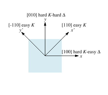
Figure 1: Anisotropies easy axes scheme of Hamiltonian (1).

The numerical simulations were performed using a Metropolis algorithm with a single spin update. The direction of each magnetic vector $\vec{S_{i}}$ is updated randomly in the unit sphere. In all the simulations we start in a random spin configuration and then cool the system with an in-plane magnetic field pointing in a given crystallographic direction. After that we cycle the field in the cooling direction to obtain the hysteresis loops.

The phase diagram of this model has been studied in the case of $\Delta=0$ and $K=0$ through Monte Carlo simulations at finite temperature Carubelli et al. (2008); Whitehead et al. (2008); Pighín et al. (2012) and analytical calculation at zero temperature Politi (1998); Yafet and Gyorgy (1988); Pighín et al. (2010). There is a region in the parameter space where the system shows a canted phase with perpendicular striped patterns. This makes the model useful to study thin film systems with a canted magnetic configuration.

In order to obtain a canted phase, we set the following parameters Pighín et al. (2010, 2012): $\eta=7$, $\mathcal{J}=6$. $K$ and $\Delta$ can be considered as small perturbations. We choose $K=0.68$ and $\Delta=0.15$. These relatively small values ensure the system remains in a canted state. We set $k_{B}T/\Omega=0.2$ in all our analyses. This is a small temperature since the ordering temperature is at least $40$ times larger. The size of the system studied is $L_{x}=L_{y}=120$.

III Results

In Fig. 2, we show vectorial hysteresis Coïsson et al. (2008) loops simulated with $K=0$ and $\Delta=0$ and the applied field in the in-plane [010] direction. This corresponds to the case where only the perpendicular uniaxial anisotropy is present, and it is a useful reference for the analysis of the main results shown in the following. One can see the typical features observed in the hysteresis loops of materials with perpendicular striped pattern with a canted magnetization, such as FePt Sallica Leva et al. (2010) or Fe_1-xGa_x Barturen et al. (2012). At high saturating fields, the magnetization is in the plane pointing in the direction of the applied field. When the field is reduced, there is a characteristic field at which stripes aligned to the field appear (see inset). From this characteristic field at which the stripes appear down to the coercivity, the magnetization inside the stripes continuously rotates. On one hand, as reflected in the vectorial hysteresis loop in Fig. 2, the in-plane rotation is marked by a linear behavior of the magnetization aligned to the field while the perpendicular in-plane magnetization increases when the field is decreased reaching its maximum value at coercivity. On the other hand, the out-of-plane magnetization goes up and down following the stripe pattern and increasing its absolute value, as can be observed through the increasing contrast of the stripes (see insets in Fig. 2).

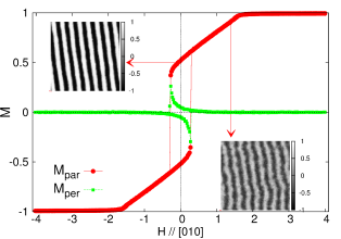
Figure 2: (Color online) Hysteresis loops with $K=0.00$, $\Delta=0.00$, $k_{B}T/\Omega=0.2$, and the field applied in the [010] direction. The snapshots show magnetic landscapes of the out of plane magnetization at remanence ($H=0$), and at $H=1.4$ close to the appearance of the stripes.

In Fig. 3, we show snapshots of the out-of-plane magnetization patterns already shown in the insets of Fig. 2 together with patterns of the in-plane magnetization parallel and perpendicular to the applied field. The upper panels correspond to $H=1.4$ and the lower panels to $H=0$, i.e. the remnant state. The white lines of Figs. 3 (c) and (f) depict the domains walls. In our convention, white means positive and black negative, i.e., along and opposite to the field, respectively. Since the in-plane magnetization perpendicular to the field –Figs. 3 (b) and (e)– does not show any preferential orientation, the domain walls are of Bloch type. The insets show the structure factor corresponding to each snapshot, defined as the squared modulus of its Fourier transform. The two peaks observed on Figs. 3 (a) and (d) account for the periodic structure and are located at the characteristic wave-vector modulus $k^{*}=2\pi/\lambda$, where $\lambda$ is the period of the stripe pattern. In our case, $\lambda=15$ and $k^{*}=0.42$. The in-plane parallel magnetization shows the presence of domain walls between two consecutive out-of-plane domains and thus has half the period of the stripe pattern. Therefore, the characteristic wave vector in Figs. 3 (c) and (f) is $2k^{*}$, as shown in the insets. Although difficult to observe under the present resolution, a weak perpendicular component can be detected in the inset of Fig. 3 (e), consistent with a Bloch domain wall (notice that the stripes are not completely vertical).

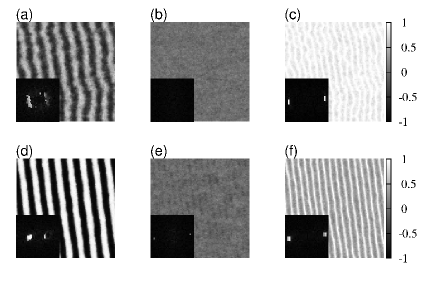
Figure 3: Snapshots of magnetic patterns corresponding to two different applied fields along the [010] in-plane direction. Top panels correspond to $H=1.4$, and bottom panels to $H=0$. (a) and (d) out-of-plane magnetization (see insets of Fig. 2), (b) and (e) in-plane magnetization perpendicular to the applied field, and (c) and (f) magnetization parallel to the applied field. Insets show the two-dimensional structure factor associated to each snapshot.

When the field is rotated and applied in the $[110]$ direction, as shown in Fig. 4, some differences can be observed as compared to Fig. 2 ($[010]$ direction). In this case, the stripes start forming with several defects and the hysteresis loop is slightly asymmetric; the descending branch being different from the ascending branch. This asymmetry can be better visualized through the hysteresis loop of the perpendicular magnetization. The slight difference between the loops in Figs. 2 and 4 arise from the spurious in-plane anisotropy introduced by lattice discretization effects in the numerical models used here. The underlying square lattice introduces a dependency of the domain-wall energy on the orientation of the stripes, which is particularly stressed in small systems. Due to this effect, the [110] direction is magnetically slightly harder than the [010] and hence domain walls aligned along the lattice directions are favored. This mechanism is behind the observed defects on the stripe patterns in Fig. 4 and is therefore responsible for the asymmetric loops.

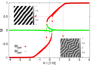
Figure 4: (Color online) Hysteresis loops with $K=0.00$, $\Delta=0.00$, $k_{B}T/\Omega=0.2$, and the field applied in the [110] direction. The snapshots show magnetic landscapes of the out of plane magnetization at remanence ($H=0$), and at $H=1.4$ close to the apparition of the stripes.

We turn now to the analysis of the effect of the cubic anisotropy. Since the cubic anisotropy term is rotated in $\pi/4$, it counteracts the lattice effects we have observed in Figs. 2 and 4. In this way, $[010]$ is a hard direction and $[110]$ is an easy direction and the lattice effect can be neglected. Interestingly, as shown in the left inset of Fig. 5, when a cubic anisotropy is added to the model ($K=0.68$), zigzags in the stripe pattern appear at remanence. In addition, at high fields, minor loops appear and we will show in the following that this is closely related to the zigzags formation. When the field is decreased from saturation, two lines of bubbles of the out-of-plane magnetization form at a field which correspond to the onset of the minor loops ($H\sim 1.4$). This magnetic configuration is shown in the upper right inset of Fig. 5. If the field is reduced to the end of the minor loops, these two lines of bubbles connect, forming undulated stripes with some defects (bottom right inset). Finally, at remanence the undulated stripes take the form of well-defined zigzags. Note that the stripe width slightly changes as the field is decreased, being it larger at remanence. This is not related to the zigzag apparition, as in the case of the mechanism proposed by Sornette, because once the stripes appear they are already undulated.

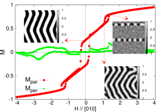
Figure 5: (Color online) Hysteresis loops with $K=0.68$, $\Delta=0.00$, $k_{B}T/\Omega=0.2$, and the field applied in the [010] direction. The snapshots show perpendicular magnetic configurations corresponding to the upper branch of the hysteresis loop: At the beginning of the minor loop ($H=1.4$), at the end ($H=1.1$), and at remanence ($H=0$).

Typical magnetic configurations associated to this process can be seen in more detail in Fig. 6. The magnetization inside the bubbles alternates in the out-of-plane direction and is canted in the direction of applied field, Figs. 6 (a) and (c), respectively. At the interface between bubbles of different orientations, the in-plane magnetization points in the direction of the applied field, small white threads in Figs. 6 (c). The in-plane magnetization perpendicular to the applied field arranges into domains (two in this case due to the size of the system) which point in opposite directions as indicated by the dark and light gray regions in Fig. 6 (b). The interface between perpendicular magnetization domains is mediated by bubble lines which can be considered as wide domain walls with a complex internal structure. The presence of these domains reduces the dipolar energy of the in plane magnetization component. Since dipolar interactions are minimized by in-plane configurations, the energy increment due to the creation of the bubble lines should be small in order to compensate the dipolar energy reduction. It is known that Bloch’s domain walls are favored in two-dimensional systems Politi (1998). Because of this fact, when the field is decreased and the stripes emerge, they follow the orientation of the in-plane magnetization. In other words, the orientation of the stripes depends on the orientation of the in-plane magnetization of the domains at which they arise. According to this, the corners of the zigzags correspond to the bubble lines, i.e., these are the lines at which stripes of different orientations connect. At zero field, Figs. 6 (d), (e) and (f), the domains of perpendicular in-plane magnetization disappear. Now, the in-plane magnetization inside the domain walls follows the orientation of the stripes. This is evidenced in Fig. 6 (e) where the in-plane component of the magnetization inside the domain walls has a different sign depending on the orientation of the stripes.

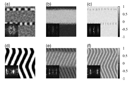
Figure 6: Snapshots of magnetic patterns corresponding to two different applied fields along the [010] in-plane direction. Top panels correspond to $H=1.4$, and bottom panels to $H=0$. (a) and (d) out-of-plane magnetization (see two top insets of Fig. 5), (b) and (e) in-plane magnetization perpendicular to the applied field, and (c) and (f) magnetization parallel to the applied field. The two-dimensional structure factor associated to each snapshot are presented in the insets, which show signatures of the different periodic structures.

Figure 7 shows hysteresis loops with the same parameters used in Fig. 5, but now the field is applied in the $[110]$ direction, i.e., the easy-$K$ direction. We see that the mechanism operating in the magnetization process from saturation to remanence is different as compared to that of the $[010]$ hard-$K$ direction. The reversible part of the loop observed after the appearance of the stripes in Figs. 2 and 5 is not present in this case. On the other hand, the in-plane magnetization perpendicular to the field is always zero, indicating that the magnetization goes to the out-of-plane direction before the inversion and does not rotate in the plane. In this applied field direction, zigzags patterns are not observed; instead, some defects like dislocations can be obtained, as the one shown at remanence (see inset of Fig. 7).

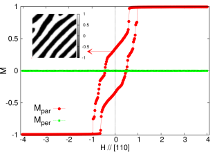
Figure 7: (Color online) Hysteresis loops obtained with $K=0.68$, $\Delta=0.00$, $k_{B}T/\Omega=0.2$. The field is applied in the $[110]$ direction. The snapshot shows perpendicular magnetic configurations corresponding to the upper branch of the hysteresis loop at remanence ($H=0$).

At this point, one might think that the symmetry between the hard-$K$ directions ($[100]$ and $[010]$) is one of the keys in the formation of the zigzag pattern. We therefore investigated whether the zigzag formation can be unfavored by a small perturbation making $[100]$ and $[010]$ directions energetically different. As shown in Fig. 8, similar hysteresis loops to those shown in Figs. 5 and 7 are found when the in-plane uniaxial anisotropy is present ($\Delta=0.15$), breaking the four-fold in-plane anisotropy of the cubic term. Now, the $[010]$ direction, along which the field is applied, is harder than the $[100]$ direction due to the presence of the $\Delta$ term; the easy-$K$ directions $[110]$ and $[-110]$ continue being equivalent (see Fig. 1). The minor loops shift toward higher fields but the phenomenology is quite similar to the one in Fig. 5, as observed in the insets. If the field is applied in $[100]$ direction, (not show here), the zigzags are still observed at remanence but its period changes. This change is related to the difference in the energy of the bubbles lines induced by the presence of uniaxial in-plane term. Finally, in this case, as in Fig. 7, when the field is applied in the $[110]$, the zigzags do not form.

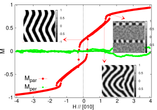
Figure 8: (Color online) Hysteresis loops obtained with $K=0.68$, $\Delta=0.15$, $k_{B}T/\Omega=0.2$, the field is applied in the [010] direction. The snapshots show perpendicular magnetic configurations corresponding to the upper branch of the hysteresis loop. At the beginning of the minor loop ($H=1.6$), at the end ($H=1.27$) and at remanence ($H=0$).

IV Anisotropy analysis

In this section, we analyze the anisotropy term of the Hamiltonian, (1), in a single spin approximation. For simplicity, we refer the cosine directors to the in-plane rotated frame, indicated by $x^{\prime}$ and $y^{\prime}$ in Fig. 1. Since we want to study the appearance of the zigzag pattern, we particularly focus on the case where the external field $H$ is oriented in the $[010]$ direction, which corresponds here to the diagonal of the $x^{\prime}-y^{\prime}$ coordinate system and thus implies an equal contribution from $\alpha_{1}$ and $\alpha_{2}$. Therefore, the single-spin anisotropy energy can be expressed as

$$E = K(\alpha_{1}^{2}\alpha_{2}^{2}+\alpha_{1}^{2}\alpha_{3}^{2}+\alpha_{2}^{2}\alpha_{3}^{2})+\frac{\Delta}{2}(\alpha_{1}+\alpha_{2})^{2}$$ (2)

$$-\frac{H}{\sqrt{2}}(\alpha_{1}+\alpha_{2})-\eta_{e}\alpha_{3}^{2},$$

where $\alpha_{i}$ are cosine directors with respect to the in-plane easy-$K$ directions (see Fig. 1) and satisfy $\alpha_{1}^{2}+\alpha_{2}^{2}+\alpha_{3}^{2}=1$. The effective uniaxial anisotropy $\eta_{e}$ takes into account the dipolar (shape anisotropy) and the uniaxial anisotropy ($\eta$) in the Hamiltonian of Eq. (1). We want to analyze the evolution with the external field $H$ of the absolute energy minima which at $H=0$ are located at $\alpha_{3}^{0}=\pm 1$ and $\alpha_{1}^{0}=\alpha_{2}^{0}=0$, i.e., with the magnetization fully oriented out of plane .

IV.1 Analysis of the critical points

From Eq. (2) and using that $1-\alpha_{1}^{2}-\alpha_{2}^{2}=\alpha_{3}^{2}$, we obtain an expression for the energy that only depends on $\alpha_{1}$ and $\alpha_{2}$:

$$E = K(\alpha_{1}^{2}+\alpha_{2}^{2}-\alpha_{1}^{2}\alpha_{2}^{2}-\alpha_{1}^{4}-\alpha_{2}^{4})+\frac{\Delta}{2}(\alpha_{1}+\alpha_{2})^{2}$$ (3)

$$-\frac{H}{\sqrt{2}}(\alpha_{1}+\alpha_{2})-\eta_{e}(1-\alpha_{1}^{2}-\alpha_{2}^{2}),$$

provided that $\alpha_{1}^{2}+\alpha_{2}^{2}\leq 1$. A graphical inspection of this energy model shows that all the minima (for the present range of parameters values) satisfy either of the following conditions: (a) $\alpha_{1}^{0}=\alpha_{2}^{0}$; (b) $\alpha_{3}^{0}=0$. The values $\alpha_{1}^{0}$ and $\alpha_{2}^{0}$ which minimize the energy model, Eq. (3), are obtained through its partial derivatives, given by

$$\frac{\partial E}{\partial\alpha_{1}} = [2K(1-\alpha_{2}^{2})+2\eta_{e}]\alpha_{1}+\Delta(\alpha_{1}+\alpha_{2})$$ (4)

$$-\frac{H}{\sqrt{2}}-4K\alpha_{1}^{3}=0,$$

$$\frac{\partial E}{\partial\alpha_{2}} = [2K(1-\alpha_{1}^{2})+2\eta_{e}]\alpha_{2}+\Delta(\alpha_{1}+\alpha_{2})$$ (5)

$$-\frac{H}{\sqrt{2}}-4K\alpha_{2}^{3}=0.$$

In order to study the stability of the solutions of this set of equations, the second derivatives of Eq. (3) should also be considered:

$$\frac{\partial^{2}E}{\partial\alpha_{1}\partial\alpha_{2}}=-4K\alpha_{1}\alpha_{2}+\Delta,$$ (6)

$$\frac{\partial^{2}E}{\partial\alpha_{1}^{2}}=2K(1-\alpha_{2}^{2})+2\eta_{e}+\Delta-12K\alpha_{1}^{2},$$ (7)

$$\frac{\partial^{2}E}{\partial\alpha_{2}^{2}}=2K(1-\alpha_{1}^{2})+2\eta_{e}+\Delta-12K\alpha_{2}^{2}.$$ (8)

In the following we analyze the solutions of Eqs. (4) and (LABEL:eg5) in order to obtain the different critical points describing the magnetization evolution observed, for example, in Fig. 5.

IV.1.1 Symmetric case: $\alpha_{1}=\alpha_{2}=\alpha$

Since when $H=0$ the energy has two absolute minima at $\alpha_{1}^{0}=\alpha_{2}^{0}=0$ and $\alpha_{3}^{0}=\pm 1$, i.e., with the magnetization perpendicular to the film plane, we expect that for small applied fields ($[010]$ direction), these minima will move in the field direction. When $\alpha_{1}=\alpha_{2}=\alpha$, Eqs. (4) and (5) reduce to the following condition:

$$P(\alpha)=-3\alpha^{3}+(1+\xi+\delta)\alpha=\frac{h}{\sqrt{8}},$$ (9)

where $\delta=\frac{\Delta}{K}$, $\xi=\frac{\eta_{e}}{K}$, and $h=\frac{H}{K}$. The solutions of the above equation are given by the intersection between the cubic polynomial $P(\alpha)$ and the horizontal line corresponding to the applied field. At $h=0$, the only stable minimum of the energy is the $\alpha^{0}=0$ solution. When $h$ increases, the value of $\alpha^{0}(H)$ corresponding to this minimum goes to positive values. Since $P(\alpha)$ has a local maximum at positive values of $\alpha$, the value of $\alpha$ at this maximum is the upper limit that $\alpha^{0}(H)$ can take as the field increases. This value is

$$\alpha_{max}=\frac{\sqrt{1+\xi+\delta}}{3}.$$ (10)

The value of the critical field necessary to be applied so the minimum of the energy is at $\alpha_{max}$ is

$$h_{1}^{*}=\frac{H_{1}^{*}}{K}=\sqrt{8}P(\alpha_{max})=\frac{4\sqrt{2}}{9}(1+\xi+\delta)^{3/2}.$$ (11)

Therefore, $\alpha^{0}(H_{1}^{*})=\alpha_{max}$ and for fields in the range $0<H<H_{1}^{*}$, the energy is minimized at $0<\alpha^{0}<\alpha^{0}(H_{1}^{*})$ and $\alpha_{3}^{0}=\pm\sqrt{1-2(\alpha^{0})^{2}}$. These solutions are represented schematically in Fig. 9 as the $A$ and $A$ points.

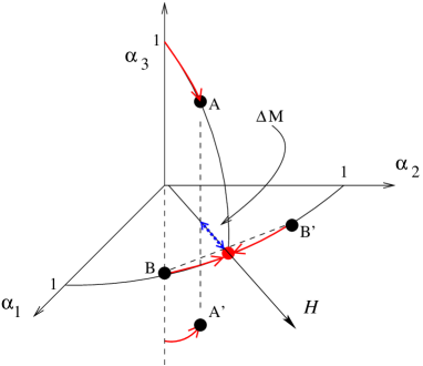
Figure 9: (Color online) Scheme of evolution of the minima with an increasing external field (red arrows). The four minima, $A$, $A^{\prime}$ and $B$, $B^{\prime}$, at the transition at $h_{1}^{*}$ are indicated with black dots. The dashed double arrow indicates the increase $\Delta M$ of the magnetization associated to the transition at $h_{1}^{*}$. At $h_{2}^{*}$ the two minima with $\alpha_{1}^{0}\neq\alpha_{2}^{0}$ collapse onto the $\alpha_{1}^{0}=\alpha_{2}^{0}=1/\sqrt{2}$ red point.

Let us analyze the stability of these minima as they move toward the direction of the applied field. The second derivatives of Eq. (3) with $\alpha_{1}=\alpha_{2}=\alpha$ are

$$\frac{\partial^{2}E}{\partial\alpha_{1}\partial\alpha_{2}}=-4K\alpha^{2}+\Delta,$$ (12)

$$\frac{\partial^{2}E}{\partial\alpha_{1}^{2}}=2(K+\eta)+\Delta-14K\alpha^{2}.$$ (13)

Using, these expressions we can obtain the Hessian. At the point where the Hessian is zero, the minimum or maximum becomes a saddle point. Two solutions are obtained:

$$\alpha_{+}=\frac{\sqrt{1+\xi}}{\sqrt{5}},$$ (14)

$$\alpha_{-}=\frac{\sqrt{1+\xi+\delta}}{3}.$$ (15)

Note that $\alpha_{-}=\alpha_{max}<\alpha_{+}$, provided that $\delta$ is small. Then, once $\alpha^{0}$ reach the value of $\alpha_{max}$ the minima become unstable.

IV.1.2 In-plane case: $\alpha_{3}=0$

As the field is increased, two other local minima with $\alpha_{1}^{0}\neq\alpha_{2}^{0}$ and $\alpha_{3}^{0}=0$ appear, namely, in-plane solutions not aligned with the field. These solutions are located symmetrically with respect to the direction of the field (see Fig.9) and we call them $B$ and $B^{\prime}$. When the solutions $A$ and $A^{\prime}$ loose stability the solutions $B$ and $B^{\prime}$ become the absolute minima. As the field further increases, the solutions $B$ and $B^{\prime}$ converges to a single one aligned with the field ($\alpha_{1}^{0}=\alpha_{2}^{0}=1/\sqrt{2}$ and $\alpha_{3}^{0}=0$).

We shall now find the critical field $h_{2}^{*}$ at which the two in-plane minima join. Taking $\alpha_{3}=0$ and $\alpha^{\prime}=\alpha_{1}=\sqrt{1-\alpha_{2}^{2}}$, Eqs. (4) and (5) reduce to

$$Q(\alpha^{\prime})= \alpha^{\prime}(1-2\alpha^{\prime 2})$$ (16)

$$+ \frac{h\alpha^{\prime}+\sqrt{2}\delta(1-2\alpha^{\prime 2})}{\sqrt{8(1-\alpha^{\prime 2})}}=\frac{h}{\sqrt{8}}.$$

This equation has three real solutions. One corresponds to $\alpha_{0}^{\prime 0}=1/\sqrt{2}$, i.e., $\alpha_{1}^{0}=\alpha_{2}^{0}=1/\sqrt{2}$. The other two symmetric solutions are $(\alpha_{1}^{0},\alpha_{2}^{0})=(\alpha_{+}^{\prime 0},\alpha_{-}^{\prime 0})$ and $(\alpha_{1}^{0},\alpha_{2}^{0})=(\alpha_{-}^{\prime 0},\alpha_{+}^{\prime 0})$, with $\alpha_{+}^{\prime 0}<1/\sqrt{2}$ and $\alpha_{-}^{\prime 0}=\sqrt{1-{\alpha_{+}^{\prime 0}}^{2}}$. For $h<h_{2}^{*}$, the solution $\alpha_{0}^{\prime 0}$ is a maximum and the other two solutions are minima. When increasing the field, these two minima converge to $\alpha_{0}^{\prime 0}$ which becomes the stable solution to Eq. (16), meaning that the magnetization is fully aligned with the external field and saturated in plane (see Fig. 9). Using the bordered Hessian matrices for the constrained extrema problem, we analyze the stability of these minima (see Appendix), and we obtain the critical field at which the two in-plane minima join:

$$h_{2}^{*}=\frac{H_{2}^{*}}{K}=2+2\delta.$$ (17)

If $h_{1}^{*}<h<h_{2}^{*}$, the two in-plane symmetric solutions exist and this is a condition for the existence of the zigzag pattern. From this condition, we obtain

$$\xi<\frac{3}{2}3^{1/3}(1+\delta)^{2/3}-(1+\delta).$$ (18)

This gives a relation between anisotropy constants $K$, $\eta_{e}$, and $\Delta$ for the existence of the zigzag pattern. In particular, for $\Delta=0$, one has that $\eta_{e}<1.16K$.

V Summary and final remarks

In the following, we shall describe the whole scenario that emerges from the previous model (Eq. (2)), and for simplicity we will focus on the case $\Delta=0$. Figure 9 shows a scheme of the energy minima in the $\alpha_{1},\alpha_{2},\alpha_{3}$ space. When $H=0$ the magnetization is fully out of plane: $\alpha_{3}^{0}=\pm 1$ and $\alpha_{1}^{0}=\alpha_{2}^{0}=0$. When increasing the field in the [010] direction, and for $0<H<H_{1}^{*}=K(1+\eta_{e}/K)^{3/2}4\sqrt{2}/9$, the magnetization still has an out-of-plane component and is canted in the direction of the field, with $|\alpha_{3}^{0}|>0$ and $\alpha_{1}^{0}=\alpha_{2}^{0}>0$. At the field $H_{1}^{*}$ the magnetization along the external field, $\alpha_{1}^{0}=\alpha_{2}^{0}$, is no longer stable and now the magnetization has two in-plane symmetric states given by $\alpha_{3}^{0}=0$ and $(\alpha_{1}^{0},\alpha_{2}^{0})=(\alpha_{+}^{\prime 0},\alpha_{-}^{\prime 0})$ and $(\alpha_{1}^{0},\alpha_{2}^{0})=(\alpha_{-}^{\prime 0},\alpha_{+}^{\prime 0})$. By further increasing the external field, the projection of these two magnetization states along the field increases until the magnetization finally aligns with the field at the value $H=H_{2}^{*}=2K$. For $H>H_{2}^{*}$, the magnetization is saturated in the direction of the external field.

When the external field is in the range $H_{1}^{*}<H<H_{2}^{*}$ there are, in the single-spin approximation, two equivalent in-plane magnetization states, not aligned with the external field. These two states can be observed in Figs. 6(b) and (c). The line of bubbles observed in Fig. 6(a) are the domain walls between the two in-plane magnetization states. The bubble structure of these domain walls is the result of the dipolar energy term, not present in the single-spin approximation, and are responsible for the origin of the zigzag pattern. At smaller external field values, $H<H_{1}^{*}$, canted magnetization states with an out-of-plane component, such as the ones in the bubbles, are favored. These are the states inside the domains observed in Figs. 6(a)–(c). The zigzag pattern then results from the connection of the bubbles when the canted states are preferred. In Fig. 10, we plot the component of the magnetization in the direction of the applied field $H$, i.e $M=(\alpha_{1}+\alpha_{2})/\sqrt{2}$. The two critical fields $H_{1}^{*}$ and $H_{2}^{*}$ are shown.

Figure 10: Evolution of the projection of the magnetization with the external field applied in the $[010]$ direction. Two curves, corresponding to $\Delta=0$ and $0.15$, are shown. The characteristic fields $H_{1}^{*}$ and $H_{2}^{*}$, as well as the increase of the in-plane magnetization $\Delta M$ at $H_{1}^{*}$, are shown.

According to the previous scenario, the fields $H_{1}^{*}$ and $H_{2}^{*}$ can be identified in the single spin model with the characteristic field values of the minor loop and the saturation field, respectively. In order to compare the predictions of the single spin approximation with the Monte Carlo simulations we choose the following set of parameters for Eq. (2): $\eta_{e}=0.72$ and $K=0.68$. With these parameters we emulate the anisotropy terms of the model Hamiltonian (Eq. (1)). As an approximation, the effective uniaxial anisotropy $\eta_{e}$ introduced in order to take into account the dipolar shape anisotropy is computed as the sum of uniaxial anisotropy $\eta$ and the effective planar dipolar anisotropy. The effective planar anisotropy correspond to the value of the anisotropy at which the system undergoes a planar to perpendicular reorientation (see Ref. Pighín et al., 2010). Note that the whole set of parameters satisfy Eq. (18). The minor loops observed in Figs. 5 and 8 are related to $H_{1}^{*}$ in the single spin model. The values of $H_{1}^{*}$ obtained as the average value between borders of the minor loops of Figs. 5 and 8 are in a very good agreement with the values obtained in the single spin model. For the cases $\Delta=0$ and $0.15$, the values $H_{1}^{*}\sim 1.25$ (Fig. 5) and $H_{1}^{*}\sim 1.47$ (Fig. 8) were obtained with numerical simulations, while the single spin model predictions for each case are $H_{1}^{*}=1.26$ and $1.47$. We see that the values predicted by the single-spin approximation for $H_{1}^{*}$ agree very well with the values coming from Monte Carlo simulations. This indicates that the chosen value for $\eta_{e}$ accurately describes the numerical data and that the single-spin approximation gives a good description of the transition occurring at $H_{1}^{*}$ and the appearance of the zigzag patterns. However, the values predicted for the saturation field $H_{2}^{*}$ do not agree with the numerical simulations. This points to the limitations of the single-spin model to take into account thermal fluctuation and also to the fact that dipolar interactions are not accurately described by an effective anisotropy when the magnetization is mainly in the plane.

Summarizing, the zigzag mechanism that emerges from the present analysis is a direct consequence of cubic anisotropy, which gives rise to two pairs of effective local minima that exchange stability as the field changes. For instance, the appearance of a bubble state depends on the ratio between the cubic anisotropy and the effective uniaxial anisotropy that takes into account dipolar energy contributions. The single absolute minimum at high fields transforms, as the field is decreased; first, in two minima with the magnetization in the film plane, and then, by a further reduction of the field, in two minima with out-of-plane magnetization. Close to the transition from two absolute minima in the plane to two absolute minima out of plane, the energies of these four minima are similar. The proximity between the energy of the minima allows the formation of bubble lines without paying so much energy, which in turn produces a reduction of the dipolar energy and the appearance of the zigzag patterns.

Appendix A Constrained critical point analysis

In this appendix we provide details of the calculations on the stability analysis of the critical points in the constrained energy problem.

Let us consider the energy $E$ and the constraint $g(\alpha_{1},\alpha_{2},\alpha_{3})=0$,

$$E = K(\alpha_{1}^{2}\alpha_{2}^{2}+\alpha_{1}^{2}\alpha_{3}^{2}+\alpha_{2}^{2}\alpha_{3}^{2})+\frac{\Delta}{2}(\alpha_{1}+\alpha_{2})^{2}$$ (19)

$$-\frac{H}{\sqrt{2}}(\alpha_{1}+\alpha_{2})-\eta_{e}\alpha_{3}^{2}$$

$$g = 1-\alpha_{1}^{2}-\alpha_{2}^{2}-\alpha_{3}^{2}=0.$$ (20)

Then the Lagrangian function $L$ of the problem is:

$$L=E-\lambda g$$ (21)

where $\lambda$ is the Lagrange multiplier. The critical points $\alpha_{1}^{*}$, $\alpha_{2}^{*}$, $\alpha_{3}^{*}$ and $\lambda^{*}$ of the Lagrangian function are solutions of the following equations:

$$\frac{\partial L}{\partial\alpha_{1}} = 2K\alpha_{1}(\alpha_{2}^{2}+\alpha_{3}^{2})+\Delta(\alpha_{1}+\alpha_{2})$$

$$-\frac{H}{\sqrt{2}}+2\lambda\alpha_{1}=0$$

$$\frac{\partial L}{\partial\alpha_{2}} = 2K\alpha_{2}(\alpha_{1}^{2}+\alpha_{3}^{2})+\Delta(\alpha_{1}+\alpha_{2})$$

$$-\frac{H}{\sqrt{2}}+2\lambda\alpha_{2}=0$$

$$\frac{\partial L}{\partial\alpha_{3}} = 2K\alpha_{3}(\alpha_{1}^{2}+\alpha_{2}^{2})-2\eta_{e}\alpha_{3}+2\lambda\alpha_{3}=0$$ (24)

$$\frac{\partial L}{\partial\lambda} = (\alpha_{1}^{2}+\alpha_{2}^{2}+\alpha_{3}^{2})-1=0$$ (25)

In order to classify the critical points, we have to analyze the determinants of the bordered Hessian matrices $H_{4}$ and $H_{3}$ evaluated at the critical points ($\alpha_{1}^{*}$, $\alpha_{2}^{*}$, $\alpha_{3}^{*}$, and $\lambda^{*}$). These matrices are:

$$H_{4}=\left(\begin{array}[]{cccc}0&-g_{x}&-g_{y}&-g_{z}\\ -g_{x}&L_{xx}&L_{xy}&L_{xz}\\ -g_{y}&L_{yx}&L_{yy}&L_{yz}\\ -g_{z}&L_{zx}&L_{zy}&L_{zz}\end{array}\right),$$ (26)

and if $g_{x}(\alpha_{1}^{*},\alpha_{2}^{*},\alpha_{3}^{*})\neq 0$ and/or $g_{y}(\alpha_{1}^{*},\alpha_{2}^{*},\alpha_{3}^{*})\neq 0$

$$H_{3}=\left(\begin{array}[]{ccc}0&-g_{x}&-g_{y}\\ -g_{x}&L_{xx}&L_{xy}\\ -g_{y}&L_{yx}&L_{yy}\end{array}\right).$$ (27)

Here, $g_{x}=\frac{\partial g}{\partial\alpha_{1}}$ , $g_{y}=\frac{\partial g}{\partial\alpha_{2}}$ and $g_{z}=\frac{\partial g}{\partial\alpha_{3}}$. Similarly, the double subscript in $L$ refers to the second partial derivatives, for instance, $L_{xy}=\frac{\partial^{2}L}{\partial\alpha_{1}\partial\alpha_{2}}$

• if $-det(H_{4})>0$ and $-det(H_{3})>0$ the critical point is a minimum.

• if $-det(H_{4})>0$ and $-det(H_{3})<0$ the critical point is a maximum.

• if $-det(H_{4})<0$ then critical point is a saddle point.

In our problem the Hessian matrices are:

$$H_{4}=\left(\begin{array}[]{cccc}0&2\alpha_{1}&2\alpha_{2}&2\alpha_{3}\\ 2\alpha_{1}&2K(\alpha_{2}^{2}+\alpha_{3}^{2})+\Delta+2\lambda&4K\alpha_{1}\alpha_{2}+\Delta&4K\alpha_{1}\alpha_{3}\\ 2\alpha_{2}&4K\alpha_{1}\alpha_{2}+\Delta&2K(\alpha_{1}^{2}+\alpha_{3}^{2})+\Delta+2\lambda&4K\alpha_{2}\alpha_{3}\\ 2\alpha_{3}&4K\alpha_{1}\alpha_{3}&4K\alpha_{2}\alpha_{3}&2K(\alpha_{1}^{2}+\alpha_{2}^{2})+2(\lambda-\eta_{e})\end{array}\right)$$ (28)

and

$$H_{3}=\left(\begin{array}[]{cccc}0&2\alpha_{1}&2\alpha_{2}\\ 2\alpha_{1}&2K(\alpha_{2}^{2}+\alpha_{3}^{2})+\Delta+2\lambda&4K\alpha_{1}\alpha_{2}+\Delta\\ 2\alpha_{2}&4K\alpha_{1}\alpha_{2}+\Delta&2K(\alpha_{1}^{2}+\alpha_{3}^{2})+\Delta+2\lambda\end{array}\right)$$ (29)

We would like to do the stability analysis for the critical point with $\alpha_{1}^{*}=\alpha_{2}^{*}=\frac{1}{\sqrt{2}}$, $\alpha_{3}^{*}=0$ and $\lambda=\lambda^{*}$. In order for this to be a critical point, and using Eq. (A) one obtains that the Lagrange multiplier is field dependent,

$$\lambda^{*}=\frac{H}{2}-\frac{K}{2}-\Delta.$$ (30)

Then evaluating the determinants of $H_{4}$ and $H_{3}$ for this critical point we obtain

$$-det(H_{4})=-det(H_{3})[H+K-2(\Delta+\eta_{e})]$$ (31)

and

$$-det(H_{3})=4[H-2(K+\Delta)]$$ (32)

Equating to zero the first and second factors in $-det(H_{4})$ we get:

$$H_{2}^{*}=2(K+\Delta)$$ (33)

$$H_{3}^{*}=2(\Delta+\eta_{e}-K/2)$$ (34)

If $\eta_{e}<\eta_{e}^{*}=3K/2$ then we are in the strong dipolar regime where $H_{3}^{*}<H_{2}^{*}$. Then,

• if $H<H_{3}^{*}$ we have that $-det(H_{4})>0$ and $-det(H_{3})<0$ and thus the critical point is a maximum,

• if $H_{3}^{*}<H<H_{2}^{*}$ then $-det(H_{4})<0$ and the critical point is a saddle point,

• if $H_{2}^{*}<H$ we have that $-det(H_{4})>0$ and $-det(H_{3})>0$ and thus the critical point is a minimum.

Since $\eta_{e}\approx K<\eta_{e}^{*}$, this is the case we are interested in and we have a well defined $H_{2}^{*}$ field value.

On the other hand, if $\eta_{e}>\eta_{e}^{*}=3K/2$ then we are in the weak dipolar regime where $H_{3}^{*}>H_{2}^{*}$. Then:

• if $H<H_{2}^{*}$ we have that $-det(H_{4})>0$ and $-det(H_{3})<0$ and thus the critical point is a maximum,

• if $H_{2}^{*}<H<H_{3}^{*}$ then $-det(H_{4})<0$ and the critical point is a saddle point,

• if $H_{3}^{*}<H$ we have that $-det(H_{4})>0$ and $-det(H_{3})>0$ and thus the critical point is a minimum.

Then, in this case we have to go beyond the field $H_{3}^{*}$ (which is larger than $H_{2}^{*}$) in order to have a minimum critical point. In this weak dipolar regime the external in-plane field has to win over the weak dipolar contribution in order to generate a fully in-plane magnetic moment.

References

- Seul and Wolfe (1992) M. Seul and R. Wolfe, Phys. Rev. A 46, 7519 (1992).
- Molho et al. (1986) P. Molho, J. Gouzerh, J. Levy, and J. Porteseil, Journal of Magnetism and Magnetic Materials 54–57, Part 2, 857 (1986), ISSN 0304-8853.
- Molho et al. (1987) P. Molho, J. L. Porteseil, Y. Souche, J. Gouzerh, and J. C. S. Levy, Journal of Applied Physics 61, 4188 (1987).
- Pappas et al. (1990) D. P. Pappas, K. P. Kamper, and H. Hopster, Phys. Rev. Lett. 64, 3179 (1990).
- Saratz et al. (2010) N. Saratz, A. Lichtenberger, O. Portmann, U. Ramsperger, A. Vindigni, and D. Pescia, Phys. Rev. Lett. 104, 077203 (2010).
- Demand et al. (2002) M. Demand, S. Padovani, M. Hehn, K. Ounadjela, and J. Bucher, Journal of Magnetism and Magnetic Materials 247, 147 (2002).
- Johansen et al. (2013) T. H. Johansen, A. V. Pan, and Y. M. Galperin, Phys. Rev. B 87, 060402 (2013).
- Sornette (1987) D. Sornette, J. Physique 48, 151 (1987).
- Coïsson et al. (2008) M. Coïsson, C. Appino, F. Celegato, A. Magni, P. Tiberto, and F. Vinai, Phys. Rev. B 77, 214404 (2008).
- Coïsson et al. (2009) M. Coïsson, F. Vinai, P. Tiberto, and F. Celegato, Journal of Magnetism and Magnetic Materials 321, 806 (2009), proceedings of the Forth Moscow International Symposium on Magnetism.
- Sallica Leva et al. (2010) E. Sallica Leva, R. C. Valente, F. Martínez Tabares, M. Vásquez Mansilla, S. Roshdestwensky, and A. Butera, Phys. Rev. B 82, 144410 (2010).
- Barturen et al. (2012) M. Barturen, B. Rache Salles, P. Schio, J. Milano, A. Butera, S. Bustingorry, C. Ramos, A. J. A. de Oliveira, M. Eddrief, E. Lacaze, et al., Applied Physics Letters 101, 092404 (2012).
- Saito et al. (1964) N. Saito, H. Fujiwara, and Y. Sugita, Journal of the Physical Society of Japan 19, 1116 (1964).
- Lo et al. (1970) D. S. Lo, D. I. Norman, and E. J. Torok, Journal of Applied Physics 41, 1342 (1970).
- Talbi et al. (2010) Y. Talbi, P. Djemia, Y. Roussigné, J. BenYoussef, N. Vukadinovic, and M. Labrune, Journal of Physics: Conference Series 200, 072107 (2010).
- Whitehead et al. (2008) J. P. Whitehead, A. B. MacIsaac, and K. De’Bell, Phys. Rev. B 77, 174415 (2008).
- Pighín et al. (2012) S. A. Pighín, O. V. Billoni, and S. A. Cannas, Phys. Rev. E 86, 051119 (2012).
- Note (1) Note1, the dipolar constant is , where is the Lande factor, the vacuum permitivity and the Bohr magneton.
- Gustavsson et al. (2002) F. Gustavsson, E. Nordström, V. H. Etgens, M. Eddrief, E. Sjöstedt, R. Wäppling, and J.-M. George, Phys. Rev. B 66, 024405 (2002).
- Carubelli et al. (2008) M. Carubelli, O. V. Billoni, S. A. Pighín, S. A. Cannas, D. A. Stariolo, and F. A. Tamarit, Phys. Rev. B 77, 134417 (2008).
- Politi (1998) P. Politi, Comments Cond. Matter Phys. 18, 191 (1998).
- Yafet and Gyorgy (1988) Y. Yafet and E. M. Gyorgy, Phys. Rev. B 38, 9145 (1988).
- Pighín et al. (2010) S. A. Pighín, O. V. Billoni, D. A. Stariolo, and S. A. Cannas, Journal of Magnetism and Magnetic Materials 322, 3889 (2010), ISSN 0304-8853.
- Note (2) Note2, in the lamellar phase with high out-of-plane anisotropy the spins inside the stripes are accommodated in this two effective minima.
- Note (3) Note3, the other two solutions of the cubic equation correspond to maxima.