DETERMINATION OF CHARGED HIGGS COUPLINGS
AT THE LHC

Abstract

We review the study of the charged Higgs and top quark associated production at the LHC with the presence of an additional scalar doublet. Top quark spin effects are related to the Higgs fermion couplings through this process. The angular distributions with respect to top quark spin turns out to be distinctive observables to study the $Htb$ interaction in different models.

PACS Nos.: 14.80.Cp,14.65.Ha,12.60.-i

1 Introduction

Gauge symmetry and electroweak spontaneous symmetry breaking (EWSB) are two fundamentals of the Standard Model (SM) of particle physics. The discovery of gauge bosons $W$ and $Z$ and further measurements established the gauge group $SU(3)_{C}\times SU(2)_{L}\times U(1)_{Y}$ of the SM. While the mechanism of EWSB is implemented by introducing one complex Higgs doublet $\Phi$ and then triggered by the development of neutral component vacuum expectation value (VEV). Weak gauge bosons and fermions get their masses in this way. In July 2012, a SM like Higgs boson with mass around 126 GeV has been discovered at the LHC by ATLAS and CMS collaborations[1, 2]. However, that introducing only one complex scalar doublet in the SM is simply based on minimal principle. It is thus natural to consider scenarios with additional complex scalars such as the two Higgs doublet model (2HDM).

Depending on Yukawa couplings between Higgs and fermions, 2HDMs are classified as different types[3, 4]. From experimental aspects, flavour changing neutral current (FCNC) should be highly suppressed at tree-level, which is realized by Glashow-Iliopoulos-Maiani (GIM) mechanism in the SM. However, in 2HDMs with extended Higgs sector, extra discrete symmetry $Z_{2}$ is usually introduced to suppress tree-level FCNC. After the spontaneous symmetry breaking, there are five physical Higgs scalars, i.e., two neutral CP-even bosons $h_{0}$ and $H_{0}$, one neutral CP-odd boson $A$, and two charged bosons $H^{\pm}$. In such models with multiple neutral scalars, the mixings between these components will make it difficult to disentangle the Higgs properties. Hence, it is important to study the charged Higgs bosons, which might be able to provide unambiguous signatures to distinguish from models with extended Higgs sector.

Constraints on the charged Higgs boson in the 2HDM are given from both collider and flavour experiments. One model-independent direct limit is from the LEP experiments, which gives $M>78.6$ GeV at 95% C.L. through exclusive decay channels of $H^{+}\to c\bar{s}$ and $H^{+}\to\tau^{+}\nu$[5], where $M$ represents the charged Higgs mass. At hadron colliders, the approaches used to search for the charged Higgs are different in the low mass region $M<m_{t}$ and in the large mass range $M>m_{t}$. When $M<m_{t}-m_{b}$, charged Higgs can be produced through the top quark decay $t\to H^{+}b$ followed by decay mode $H^{+}\to\bar{\tau}\nu$. On the other hand, when $M>m_{t}+m_{b}$, the dominant production process through gluon bottom fusion $gb\to tH^{-}$, followed by dominant decay modes $H^{-}\to t\bar{b}$ and $H^{-}\to\tau\bar{\nu}$. The Tevatron constrains 2HDM for a charged Higgs boson with the lower bound as $\sim 160$ GeV [6, 7, 8, 9]. In addition, the indirect flavour constraints can be extracted from B-meson decays since the charged Higgs contributes to the FCNC process. In Type-II 2HDM, a lower limit on the charged Higgs mass $M>316~{}{\rm GeV}$ at $95\%$ C.L. is obtained mainly from $b\to s\gamma$ branching ratio measurement irrespective of the value of $\tan\beta$ [10, 11]. However, in Type-III or general 2HDM the phases of the Yukawa couplings are free parameters so that $M$ is less constrained and can be as low as 100 GeV[12, 13]. For more detailed discussions on phenomenological constraints on charged Higgs, we refer to Ref. 14.

Along with the experimental search for the charged Higgs boson, there are also extensive phenomenological studies on charged Higgs boson production at the LHC [15, 16, 17, 18, 19, 20, 21, 22, 23, 24, 25, 28, 29, 26, 27, 30, 31, 32]. Especially, the gluon bottom fusion process $gb\rightarrow tH^{-}$ for the charged Higgs mass $M>m_{t}+m_{b}$ shows a lot of interesting signatures due to the large couplings of $Htb$ interaction [22, 25, 28, 29, 30, 32, 33]. The next-to-leading order QCD corrections to this process has also been performed in Ref. 34-37.

In this Letter, we revisit the process $gb\rightarrow tH^{-}$ at the LHC and take a method similar to Ref. 38, 39 to optimize this signal from the SM backgrounds. As claimed in Ref. 38, the angular distribution related to top quark spin is efficient to disentangle the chiral coupling of the $W^{\prime}$ boson to the SM fermions. The left-right asymmetry induced by top quark spin for the process $pp\to tH^{-}$ has been analyzed in Ref. 40, 41. Here we further investigate such a kind of effect after including the charged Higgs and top quark decay, and we employ the angular distributions of the top quark and the final state leptons to disentangle $Htb$ couplings at LHC.

The following discussions are organized as follows. In Section 2., the corresponding theoretical framework is briefly introduced. In Section 3, we perform the numerical analysis of top quark and charged Higgs associated production process from the gluon bottom fusion. Specifically, the correlated angular distributions of the final state particles are investigated to identify the interaction of top-bottom quark and charged Higgs. Finally, summary and discussions are given in Section 4.

2 Theoretical Framework

2.1 The Lagrangian and constraints on the model parameters

To begin with, we give a brief introduction to the two-Higgs-Doublet Models (2HDMs), which is one of the minimal extensions of the SM. Different from the SM with only one scalar doublet, two complex ${SU(2)_{L}}$ doublet scalar fields are introduced in the 2HDMs, which can be written as

$$\Phi_{i}=\left(\begin{array}[]{c}H_{i}^{+}\\ (H_{i}^{0}+iA_{i}^{0})/\sqrt{2}\end{array}\right),$$ (1)

where $i=1,2$. Imposing CP invariance and ${\rm U(1)_{EM}}$ gauge symmetry, the minimization of potential gives

$$\langle\Phi_{i}\rangle=\displaystyle{\frac{1}{\sqrt{2}}}\left(\begin{array}[]{c}0\\ v_{i}\end{array}\right),$$ (4)

with $v_{i}~{}(i=1,2)$ is non-zero vev. After the spontaneous symmetry breaking, there are five physical Higgs scalars, i.e., two neutral CP-even bosons $h_{0}$ and $H_{0}$, one neutral CP-odd boson $A$, and two charged bosons $H^{\pm}$. The ratio between the vets of the two scalar doublets is defined as ${\displaystyle{\tan\beta\equiv{v_{2}}/{v_{1}}}}$, which determines the interactions of the Higgs fields with the vector bosons and fermions. For simplicity, the masses of these Higgs bosons are assumed to be degenerate.

Since phenomenologies from charged Higgs are possible to shed some lights on the extended Higgs sector, in the following we aim to study the charged Higgs signatures at the LHC in the framework of the Type II 2HDM Yukawa couplings,

$$-\mathcal{L} = -\cot\beta\frac{m_{u}}{v}\bar{u}_{L}(H+iA)u_{R}+\tan\beta\frac{m_{d}}{v}\bar{d}_{L}(H-iA)d_{R}$$ (5)

$$-\sqrt{2}\cot\beta\frac{m_{u}}{v}V_{ud}^{{\dagger}}\bar{d}_{L}H^{-}u_{R}-\sqrt{2}\tan\beta\frac{m_{d}}{v}V_{ud}\bar{u}_{L}H^{+}d_{R}+{\rm h.c.}.$$

The VEV of the SM Higgs is related as $v=\sqrt{v_{1}^{2}+v_{2}^{2}}$. Following the Ref. 3, $t\bar{b}H^{-}$ coupling can be written as

$$g_{H^{-}t\bar{b}} = g_{a}+g_{b}\gamma_{5}.$$ (6)

Within the Type-II 2HDM,

$$g_{a,b}=g({\rm cot}\beta m_{t}\pm{\rm tan}\beta m_{b})/(2\sqrt{2}m_{{\rm W}}).$$

We can also define $g_{L}$ and $g_{R}$

$$-\mathcal{L} = g_{L}\bar{t}_{R}b_{L}H^{+}+g_{R}\bar{t}_{L}b_{R}H^{+}+{\rm h.c.}$$

$$= \left(g_{L}\bar{t}\frac{1-\gamma_{5}}{2}b+g_{R}\bar{t}\frac{1+\gamma_{5}}{2}b\right)H^{+}+{\rm h.c.}$$

$$= \bar{t}\left(\frac{g_{L}+g_{R}}{2}+\frac{g_{L}-g_{R}}{2}\right)bH^{+}+{\rm h.c.}$$

$$= \bar{t}\left(g_{a}+g_{b}\right)bH^{+}+{\rm h.c.}$$

Behaviours of coupling constants $g_{L}$, $g_{R}$, $g_{a}$ and $g_{b}$ are shown versus $\tan\beta$ in Fig. 1. We can see that the value of $g_{a}g_{b}$ becomes minus around $\tan\beta\approx 7\approx\sqrt{\frac{m_{t}}{m_{b}}}$, while $g_{a}g_{b}>0$ corresponds to $\tan\beta<7$, and $g_{a}g_{b}<0$ corresponds to $\tan\beta>7$.

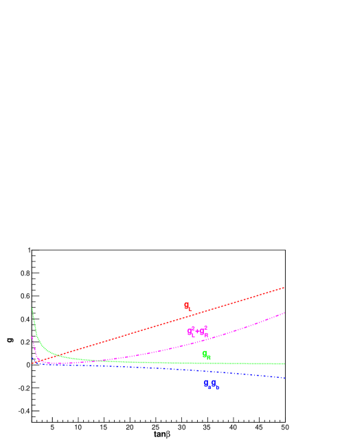
Figure 1: Couplings $g_{L}$, $g_{R}$, $g_{L}^{2}+g_{R}^{2}$ and $g_{a}g_{b}=\frac{g_{R}^{2}-g_{L}^{2}}{4}$ versus $\tan\beta$.

2.2 $tH^{-}$ associated production at the LHC

We begin to consider the following process of charged Higgs production, and the Feynman diagrams are illustrated in Fig. 2.

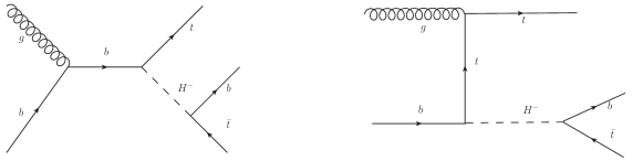
Figure 2: Feynman diagrams for $gb\to tH^{-}\to t\bar{t}b$ process.

$$g(p_{1})+b(p_{2}) \to t(p_{3},s_{t})+H^{-}(p_{4})$$ (8)

$$\to t(p_{3},s_{t})+b(p_{5})+\bar{t}(p_{6},s_{\bar{t}}),$$

where $p_{i}$ is the four-momentum of the corresponding particle. $s_{t}$($s_{\bar{t}}$) is the top (antitop) quark spin vector in 4-dimension with $s_{t}^{2}=s_{\bar{t}}^{2}=-1$ and $p_{3}\cdot s_{t}=p_{6}\cdot s_{\bar{t}}=0$.

When the charged Higgs is produced on-shell , under the narrow width approximation, we have

$$\lim_{\Gamma\to 0}\frac{1}{(p_{4}^{2}-M^{2})^{2}+\Gamma^{2}M^{2}}\longrightarrow\frac{\pi}{\Gamma M}\,\delta(p_{4}^{2}-M^{2}),$$ (9)

where $\Gamma$ and $M$ represent the charged Higgs boson decay width and mass, respectively. The squared matrix element for the process (8) including top quark spin information can be written as

$$|{\cal M}(s_{t},s_{\bar{t}})|^{2}= |{\cal M}_{gb\to tH^{-}}(s_{t})|^{2}|{\cal M}_{H^{-}\to b\bar{t}}(s_{\bar{t}})|^{2}\times\frac{\pi}{\Gamma M}\delta(p_{4}^{2}-M^{2}),$$

where

$$|{\cal M}_{gb\to tH^{-}}(s_{t})|^{2}=\frac{g_{s}^{2}}{2N_{c}}\Big{\{}{\cal A}+{\cal B}_{1}(p_{1}\cdot s_{t})+{\cal B}_{2}(p_{2}\cdot s_{\bar{t}})\Big{\}},$$ (10)

and

$$|{\cal M}_{H^{-}\to b\bar{t}}(s_{\bar{t}})|^{2} = (g_{a}^{2}+g_{b}^{2})(M^{2}-m_{b}^{2}-m_{t}^{2})-2(g_{a}^{2}-g_{b}^{2})m_{b}m_{t}$$ (11)

$$-4g_{a}g_{b}m_{t}(p_{5}\cdot s_{\bar{t}}).$$

The expressions of ${\cal A}$, ${\cal B}_{1}$ and ${\cal B}_{2}$ are

$${\cal A}=(g_{a}^{2}+g_{b}^{2})\,A_{1}\,+\,m_{b}m_{t}(g_{b}^{2}-g_{a}^{2})\,A_{2},$$ (12)

with

$$A_{1} = \displaystyle{\frac{\hat{s}(p_{1}\cdot p_{3})-m_{b}^{2}(4p_{1}\cdot p_{3}+3p_{2}\cdot p_{3})}{(\hat{s}-m_{b}^{2})^{2}}}+\frac{\hat{s}(p_{1}\cdot p_{3})+m_{t}^{2}(\hat{s}-2p_{2}\cdot p_{3})}{4(p_{1}\cdot p_{3})^{2}}$$ (13)

$$-\frac{1}{2(p_{1}\cdot p_{3})(\hat{s}-m_{b}^{2})}\big{\{}m_{t}^{2}(\hat{s}-2m_{b}^{2})-2(p_{1}\cdot p_{3})m_{b}^{2}$$

$$+2(\hat{s}-2p_{2}\cdot p_{3})(p_{1}\cdot p_{3}+p_{2}\cdot p_{3})\big{\}},$$

$$A_{2} = \frac{(\hat{s}+2m_{b}^{2})}{(\hat{s}-m_{b}^{2})^{2}}+\frac{m_{t}^{2}-p_{1}\cdot p_{3}}{2(p_{1}\cdot p_{3})^{2}}-\frac{2p_{1}\cdot p_{3}+4p_{2}\cdot p_{3}-\hat{s}}{2(p_{1}\cdot p_{3})(\hat{s}-m_{b}^{2})},$$ (14)

and

$$B_{1} = 2g_{a}g_{b}m_{t}[\frac{4m_{b}^{2}-\hat{s}}{(\hat{s}-m_{b}^{2})^{2}}+\frac{2p_{2}\cdot p_{3}-\hat{s}}{4(p_{1}\cdot p_{3})^{2}}+\frac{1}{p_{1}\cdot p_{3}}-\frac{p_{2}\cdot p_{3}}{(p_{1}\cdot p_{3})(\hat{s}-m_{b}^{2})}],$$ (15)

$$B_{2} = 2g_{a}g_{b}m_{t}[\frac{3m_{b}^{2}}{(\hat{s}-m_{b}^{2})^{2}}+\frac{m_{t}^{2}-p_{1}\cdot p_{3}}{2(p_{1}\cdot p_{3})^{2}}\frac{\hat{s}-p_{1}\cdot p_{3}-2p_{2}\cdot p_{3}}{(p_{1}\cdot p_{3})(\hat{s}-m_{b}^{2})}].$$ (16)

The similar results can be obtained for the process $g\bar{b}\to\bar{t}H^{+}\to t\bar{t}\bar{b}$ from the above equations by using CP-invariance. We can see that the top quark spin effects are related to the product of $g_{a}g_{b}$ while disappear for a pure scalar or pseudo-scalar charged Higgs boson. For $pp\to tH^{-}\to t\bar{t}b$ process, this feature can be reflected by the following spin observable

$$<{\cal{O}}_{t}>=2<\bf{{S_{t}}}\cdot{\bf\hat{a}}>={\sigma(\uparrow)-\sigma(\downarrow)\over\sigma(\uparrow)+\sigma(\downarrow)},\\$$ (17)

where $\bf{{S_{t}}}$ is the top quark spin vector in its own rest frame, and the arrows on the right-hand side refer to the spin state of the top quark corresponding to the quantization unit axis ${\bf\hat{a}}$. At the LHC, the helicity basis serves a better choice, i.e., ${\bf\hat{a}}={\bf{\hat{p}}}_{t}^{*}$ with the 3-momentum unit vector ${\bf{\hat{p}}}_{t}^{*}$ in the $tH^{-}$ center-of-mass frame. We can also define the spin observable of antitop quark in a similar way

$$<{\cal{O}}_{\bar{t}}>=2<\bf{{S}_{\bar{t}}}\cdot{\bf\hat{b}}>,$$ (18)

where $\bf{\hat{b}}$ is the spin quantization axis corresponding to antitop quark. At the LHC, we can choose ${\bf\hat{b}}={\bf{\hat{p}}}_{\bar{t}}^{*}$ with the 3-momentum unit vector ${\bf{\hat{p}}}_{\bar{t}}^{*}$ in the charged Higgs rest frame.

For the polarized top quark decay

$$t({\bf{S_{t}}})\to c(p_{c})+X,$$

where $c$ represents a final state particle or jet and $p_{c}$ represents its four-momentum, the corresponding differential distribution can be written as[42]

$$\frac{1}{\Gamma_{t}}\frac{d\Gamma_{t}}{d\cos\vartheta}=\frac{1}{2}\left(1+\kappa_{c}\cos\vartheta\right),$$ (19)

where $\vartheta$ is the angle between the top quark spin vector and the direction of $c$ in the top quark rest frame. $\kappa_{c}$ is the spin analysing power of the corresponding particle or jet $c$. For the charged lepton from the semileptonic top quark decay within SM, we have $\kappa_{l^{+}}=1$ at the tree level.

3 Numerical Results and discussion

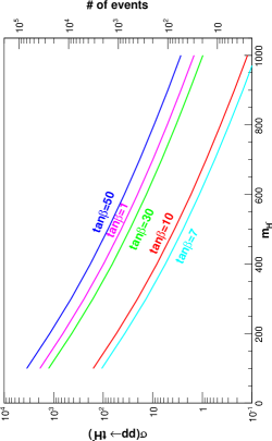
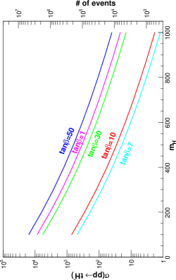
Figure 3: The cross section and number of events for signal process $pp\to tH^{-}$ at centre of mass energy 8 TeV LHC with luminosity 20$fb^{-1}$ (left panel) and centre of mass energy 14 TeV LHC with luminosity 300$fb^{-1}$ (right panel).

In Fig. 3, the total cross sections and number of events for $pp\to tH^{-}$ are shown as a function of charged Higgs mass for $\tan\beta=1,7,10$, 30, and 50 in 2HDM at the LHC with 8 TeV and 14 TeV. With assumed integrated luminosity to be 20 fb^-1 for 8 TeV and 300 fb^-1 for 14 TeV, it is shown that there are significant number of events for charged Higgs mass up to 1 TeV. Considering the decay modes of the top quark, we investigate the processes

$$pp\to tH^{-}\,\to\,t\bar{t}b\,\to\,bl^{+}\,+\,b\bar{b}jj\,+\,\displaystyle{\not}E_{T},$$ (20)

$$pp\to tH^{-}\,\to\,t\bar{t}b\,\to\,bjj\,+\,b\bar{b}l^{-}\,+\,\displaystyle{\not}E_{T}.$$ (21)

In process (20), the top quark produced associated with $H^{-}$ decays semi-leptonically, and the anti-top quark from charged Higgs decays hadronically, i.e., $t\to bl^{+}\nu_{l}$ and $\bar{t}\to\bar{b}jj$. While in process (21), ${t}\to{b}jj$ and $\bar{t}\to\bar{b}l^{-}\bar{\nu}_{l}$. The dominant SM background process is from $pp\to t\bar{t}j$. To be more realistic, the simulation at the detector is performed by smearing the energies of final state leptons and jets, according to the assumption of the Gaussian resolution parameterization

For our signal process, one of the top quarks which decays hadronically can be reconstructed from the final state three jets. However, to reconstruct another top which decays leptonically, we have to utilize kinematical constraints to reconstruct its four-momentum because of the missing energy from neutrinos. The transverse momentum of neutrino can be obtained by momentum conservation from the observed particles

$${\bf p}_{\nu T}=-({\bf p}_{lT}+\sum_{j=1}^{5}{\bf p}_{jT}),$$ (22)

while its longitudinal momentum can not be determined in this way due to the unknown boost of the partonic centre-of-mass system. Alternatively, it can be solved with twofold ambiguity through the on-shell condition of the W boson

$$m_{W}^{2}=(p_{\nu}+p_{l})^{2}.$$ (23)

Furthermore one can remove the ambiguity through the reconstruction of the other top quark. We thus evaluate the invariant mass for each possibility

$$M_{jl\nu}^{2}=(p_{l}+p_{\nu}+p_{j})^{2},$$ (24)

where $j$ refers to the any one of the two left jets and pick up the solution which is the closest to the top quark mass. With such a solution, we can reconstruct the four-momentum of the neutrino and that of the left top quark.

Therefore, in the following numerical calculations, we apply the basic acceptance cuts (cut I)

$$p_{lT}>20~{}{\rm GeV},~{}~{}~{}~{}p_{jT}>20~{}{\rm GeV},~{}~{}~{}~{}\displaystyle{\not}E_{T}>20~{}{\rm GeV},$$

$$|\eta_{l}|<2.5,~{}~{}~{}~{}|\eta_{j}|<2.5,~{}~{}~{}~{}\Delta R_{jj(lj)}>0.4,$$

$$|M_{j_{a}l\nu}-m_{t}|\leq 30~{}{\rm GeV},~{}~{}~{}~{}|M_{j_{b}j_{c}j_{d}}-m_{t}|\leq 30~{}{\rm GeV},$$

$$|M_{j_{b}j_{c}}-m_{W}|<10~{}{\rm GeV}.$$ (25)

After smearing and including the cut, the events were fully reconstructed , we can further reconstruct the invariant mass between the reconstructed top (antitop) and the remaining jet. We display the distributions $1/\sigma(d\sigma/dM_{tb}+d\sigma/dM_{\bar{t}b})$ in Fig. 4, where the resonance peaks are shown for different charged Higgs masses. According to these resonance peaks we further employ a second cut (cut II)

Figure 4: The invariant mass distributions $1/\sigma(d\sigma/dM_{tb}+d\sigma/dM_{\bar{t}b})$. $M_{tb}(M_{\bar{t}b})$ is the invariant mass between the reconstructed top (antitop) and the remaining jet for the process of $pp\to tH^{-}\to l^{+}+5jets+\displaystyle{\not}E_{T}$ after cut I at LHC for (a) 8 TeV and (b) 14 TeV.

• Cut II: $|M_{jj_{b}j_{c}j_{d}}-M|\leq 10\%\,M$ or $|M_{jj_{a}l\nu}-M|\leq 10\%\,M$.

Comparing our signal process with the dominant background process $pp\to t\bar{t}j$, after reconstructing the top and antitop quarks, the remaining jet is a b-jet for our signal while it would probably be a light jet for the SM background process. Therefore, we adopt the following cut ( cut III)

• Cut III: We demand the only remaining jet to be a b-jet.

The efficiency of $b$-tagging is assumed to be 60% while the miss-tagging efficiency of a light jet as a $b$ jet is taken to be transverse momentum dependent accordingly[43].

The cross sections and number of events for the signal and background processes (20) and (21) with different charged Higgs mass after each cut at the LHC run of 8 TeV with integrated luminosity as 20 fb^-1 and 14 TeV with integrated luminosity as 300 fb ^-1 are respectively listed in Table. 3. The dominant SM background is $pp\to t\bar{t}j\to l^{\pm}+5jets+\displaystyle{\not}E_{T}$ process. At the LHC run of $\sqrt{s}=8$ TeV, we can see that it is difficult to detect such final states from $tH^{\pm}$ production when charged Higgs mass is above 500 GeV. While with $300fb^{-1}$ integrated luminosity at 14 TeV, the significance can also be above three sigma for the charged Higgs mass $M\leq 1$ TeV. In the following, we will focus on the $tH^{-}$ production at $\sqrt{s}=14$ TeV.

The number of events of the signal process $pp\to tH^{-}\to l^{\pm}+5jets+\displaystyle{\not}E_{T}$ and the background process of $pp\to t\bar{t}j\to l^{\pm}+5jets+\displaystyle{\not}E_{T}$ at $\sqrt{s}=8$ TeV(left) and 14 TeV (right) before and after each cut.  Signal $\sigma(pp\to tH^{-}\to t\bar{t}b\to l^{\pm}+5jets+\displaystyle{\not}E_{T})$ $M$(TeV) 0.3 0.5 0.8 1.0 No cuts 903.6 172.4 20.4 6 Cut I 234.4 44 5 1.4 +Cut II 191.8 34.6 4 1 +Cut III 115.2 20.8 2.4 0.6 Background $\sigma(pp\to t\bar{t}j\to l^{\pm}+5jets+\displaystyle{\not}E_{T})$ Cuts I+II+III 205 77 19.4 9.2 $S/B$ 0.56 0.27 0.12 0.07 $S/\sqrt{S+B}$ 6.43 2.10 0.51 0.19  Signal $\sigma(pp\to tH^{-}\to t\bar{t}b\to l^{\pm}+5jets+\displaystyle{\not}E_{T})$ $M$(TeV) 0.3 0.5 0.8 1.0 No cuts 78846 19788 3468 1284 Cut I 19737 4923 825 285 +Cut II 16236 3900 660 231 +Cut III 9741 2340 396 138 Background $\sigma(pp\to t\bar{t}j\to l^{\pm}+5jets+\displaystyle{\not}E_{T})$ Cuts I+II+III 13062 5691 1785 966 $S/B$ 0.75 0.41 0.22 0.14 $S/\sqrt{S+B}$ 64.5 26.1 8.48 4.15

From Eqs. (10) and (11), we can see that the top quark spin effect is related to the product of $g_{a}g_{b}$. Using the same method as in Ref. 44 - 46, we find that this effect can be translated into the angular distributions of the charged lepton. According to the (20) and (21), we obtain the angular distributions

$$\frac{1}{\sigma}\,\frac{d\sigma}{d\cos\theta^{*}}\,=\,\frac{1}{2}\,[1\,+\,A_{FB}\cos\theta^{*}],~{}~{}~{}~{}\frac{1}{\sigma}\,\frac{d\sigma}{d\cos\bar{\theta}^{*}}\,=\,\frac{1}{2}\,[1\,+\,\bar{A}_{FB}\cos\bar{\theta}^{*}],$$ (26)

with

$$\cos\theta^{*}={{\bf\hat{p}}_{l^{+}}^{*}\cdot{\bf\hat{p}}_{t}^{*}},~{}~{}~{}~{}~{}\cos\bar{\theta}^{*}={{\bf\hat{p}}_{l^{-}}^{*}\cdot{\bf\hat{p}}_{\bar{t}}^{*}},$$ (27)

where ${\bf\hat{p}}_{l^{+}}^{*}$ is the 3-momentum unit vector of charged lepton in the top quark rest frame, and ${\bf\hat{p}}_{l^{-}}^{*}$ is the 3-momentum unit vector of charged lepton in the antitop quark rest frame. Without smearing effect and any acceptance cuts, $A_{FB}$($\bar{A}_{FB}$) can be related to the top quark spin observables ${\cal{O}}_{t}$(${\cal{O}}_{\bar{t}}$), i.e.,

$$A_{FB}=\kappa_{c}<{\cal O}_{t}>=2\kappa_{c}<\bf{{S_{t}}}\cdot{\bf\hat{p}}_{t}^{*}>,\bar{A}_{FB}=\kappa_{c}<{\cal O}_{\bar{t}}>=2\kappa_{c}<\bf{{S}_{\bar{t}}}\cdot{\bf\hat{p}}_{\bar{t}}^{*}>.$$ (28)

Thus, for the charged lepton from semileptonic top quark decay, $A_{FB}=<{\cal O}_{t}>$ and $\bar{A}_{FB}=<{\cal O}_{\bar{t}}>$ before smearing effect and cuts.

According to Eq.(26), $A_{FB}$ and $\bar{A}_{FB}$ can also be determined as follows

$$A_{FB}=\frac{\sigma(\cos\theta^{*}>0)-\sigma(\cos\theta^{*}<0)}{\sigma(\cos\theta^{*}>0)+\sigma(\cos\theta^{*}<0)},\bar{A}_{FB}=\frac{\sigma(\cos\bar{\theta}^{*}>0)-\sigma(\cos\bar{\theta}^{*}<0)}{\sigma(\cos\bar{\theta^{*}}>0)+\sigma(\cos\bar{\theta}^{*}<0)}.$$ (29)

These observables are useful to discriminate $Htb$ interactions from different models. In the framework of Type II 2HDM, the form of the Yukawa coupling is determined by only one free parameter $\tan\beta$. Combining the results of the $tH^{-}$ production cross section together with the forward-backward asymmetry $A_{FB}$ and $\bar{A}_{FB}$, one can subtract the information of $\tan\beta$ related to the $Htb$ coupling. Furthremore, we extend our discussions in a general model where the Yukawa coupling of the charged Higgs bosons to fermions is a free parameter so one can regard the scalar and pseudo-scalar parts of the Yukawa coupling as completely independent and free parameters. In the following, as an example, we choose $\tan\beta=30$ and investigate the charged lepton angular distributions for three different combinations of $g_{a}g_{b}$:

• $g_{a}g_{b}>0$, e.g.,
  $g_{a}=\pm g({\rm cot}\beta m_{t}+{\rm tan}\beta m_{b})/(2\sqrt{2}m_{{\rm W}})$,
  $g_{b}=\pm g(\cot\beta m_{t}-\tan\beta m_{b})/(2\sqrt{2}m_{{\rm W}})$.

• $g_{a}g_{b}=0$, e.g.,
  $g_{a}=0$, $g_{b}=g(\cot\beta m_{t}-\tan\beta m_{b})/(2\sqrt{2}m_{{\rm W}})$ or
  $g_{a}=g({\rm cot}\beta m_{t}+{\rm tan}\beta m_{b})/(2\sqrt{2}m_{{\rm W}})$, $g_{b}=0$.

• $g_{a}g_{b}<0$, e.g.,
  $g_{a}=\pm g({\rm cot}\beta m_{t}+{\rm tan}\beta m_{b})/(2\sqrt{2}m_{{\rm W}})$,
  $g_{b}=\mp g(\cot\beta m_{t}-\tan\beta m_{b})/(2\sqrt{2}m_{{\rm W}})$.

The predictions for $A_{FB}$ and $\bar{A}_{FB}$ corresponding to $g_{a}g_{b}$ are listed in Table 3. Because the cross section contribution from the $s$-channel(Fig.2(a)) decreases as the charged Higgs mass increases, without kinematical cuts, the $\cos\theta^{*}$ distribution and the $A_{FB}$ which are related to $tH^{-}$ production also depend on $M$; while the $\cos\bar{\theta}^{*}$ distribution and the $\bar{A}_{FB}$ which are related to the charged Higgs decay becomes $M$ independent. More specific results can be found in Ref 47. From our study, after the acceptance cuts, the angular distribution with respect to $\cos\theta^{*}$($\cos\bar{\theta}^{*}$) and $A_{FB}$($\bar{A}_{FB}$) is more helpful to investigate the $Htb$ interaction for light(heavy) charged Higgs production associated with top quark at the LHC.

The forward-backward asymmetry $A_{FB}$($\bar{A}_{FB}$) for $pp\to tH^{-}\to l^{+}(l^{-})+5jets+\displaystyle{\not}E_{T}$ at LHC $\sqrt{s}=14$ TeV before and after all cuts. $A_{FB}$ $\bar{A}_{FB}$ without cuts and smearing effect $M$(TeV) 0.3 0.5 0.8 1.0 0.3 0.5 0.8 1.0 $(g_{a}g_{b})>0$ 0.124 0.075 0.023 -0.003 -0.173 -0.173 -0.172 -0.173 $(g_{a}g_{b})=0$ 0.0 0.0 0.0 0.0 0.0 0.0 0.0 0.0 $(g_{a}g_{b})<0$ -0.125 -0.076 -0.024 0.001 0.172 0.173 0.174 0.173 with cuts and smearing effect $(g_{a}g_{b})>0$ 0.002 -0.015 -0.031 -0.041 -0.014 -0.050 -0.054 -0.061 $(g_{a}g_{b})=0$ -0.028 -0.030 -0.033 -0.041 -0.022 0.007 0.006 -0.006 $(g_{a}g_{b})<0$ -0.056 -0.048 -0.037 -0.040 -0.033 0.081 0.077 0.065

4 Summary

The observation of the charged Higgs is very important as an unambiguous signal for the existence of new physics beyond SM. Therefore it is necessary to study the related phenomena both theoretically and experimentally. In this letter, we study the determination of charged Higgs coupling of the $tH^{-}$ associated production via $pp\to tH^{-}\to t\bar{t}b\to l^{\pm}+bb\bar{b}jj+\displaystyle{\not}E_{T}$ process at LHC. We find that with 300 $fb^{-1}$ integral luminosity at $\sqrt{s}=14$ TeV, the signal can be distinguished from the backgrounds for the charged Higgs mass up to 1 TeV or even larger. If the $tH^{-}$ production is observed at the LHC, one of the following questions is to identify the $Htb$ interaction. For this purpose, we study the angular distributions of the charged leptons and the corresponding forward-backward asymmetry induced by top quark spin. It is found that these distributions and observables are sensitive to the product of $g_{a}g_{b}$, so that they can be used to identify the $Htb$ interaction. The $Htb$ interaction can be discriminated with the help of the charged lepton angular distribution and the forward-backward asymmetry in the charged Higgs and top quark associated production at the LHC. Similar methods have also been proposed using such observables related to the top quark  [48, 49]. These analyses are helpful to distinguish the $Htb$ interaction in the 2HDM or other new physics models with the presence of the charged Higgs.

References

- [1] G. Aad et al. [ATLAS Collaboration], Phys. Lett. B 716, 1 (2012) [arXiv:1207.7214 [hep-ex]].
- [2] S. Chatrchyan et al. [CMS Collaboration], Phys. Lett. B 716, 30 (2012) [arXiv:1207.7235 [hep-ex]].
- [3] J. F. Gunion, H. E. Haber, G. L. Kane and S. Dawson, Front. Phys. 80, 1 (2000).
- [4] G. C. Branco, P. M. Ferreira, L. Lavoura, M. N. Rebelo, M. Sher and J. P. Silva, Phys. Rept. 516, 1 (2012) [arXiv:1106.0034 [hep-ph]].
- [5] [LEP Higgs Working Group for Higgs boson searches and ALEPH and DELPHI and L3 and OPAL Collaborations], hep-ex/0107031.
- [6] A. Abulencia et al. [CDF Collaboration], Phys. Rev. Lett. 96, 042003 (2006) [hep-ex/0510065];
- [7] V. M. Abazov et al. [D0 Collaboration], Phys. Lett. B 682, 278 (2009) [arXiv:0908.1811 [hep-ex]];
- [8] T. Aaltonen et al. [CDF Collaboration], Phys. Rev. Lett. 103, 101803 (2009) [arXiv:0907.1269 [hep-ex]];
- [9] V. M. Abazov et al. [D0 Collaboration], Phys. Rev. D 80, 051107 (2009) [arXiv:0906.5326 [hep-ex]].
- [10] O. Deschamps, S. Descotes-Genon, S. Monteil, V. Niess, S. T’Jampens and V. Tisserand, Phys. Rev. D 82, 073012 (2010) [arXiv:0907.5135 [hep-ph]].
- [11] F. Mahmoudi and O. Stal, Phys. Rev. D 81, 035016 (2010) [arXiv:0907.1791 [hep-ph]].
- [12] V. D. Barger, M. S. Berger and R. J. N. Phillips, Phys. Rev. Lett. 70, 1368 (1993) [hep-ph/9211260].
- [13] S. -S. Bao, F. Su, Y. -L. Wu and C. Zhuang, Phys. Rev. D 77, 095004 (2008) [arXiv:0801.2596 [hep-ph]].
- [14] J. Beringer et al. [Particle Data Group Collaboration], Phys. Rev. D 86, 010001 (2012).
- [15] E. Eichten, I. Hinchliffe, K. D. Lane and C. Quigg, Rev. Mod. Phys. 56, 579 (1984) [Addendum-ibid. 58, 1065 (1986)].
- [16] N. G. Deshpande, X. Tata and D. A. Dicus, Phys. Rev. D 29, 1527 (1984).
- [17] S. S. D. Willenbrock, Phys. Rev. D 35, 173 (1987).
- [18] A. Krause, T. Plehn, M. Spira and P. M. Zerwas, Nucl. Phys. B 519, 85 (1998) [hep-ph/9707430].
- [19] A. A. Barrientos Bendezu and B. A. Kniehl, Phys. Rev. D 59, 015009 (1999) [hep-ph/9807480];
- [20] S. Moretti and K. Odagiri, Phys. Rev. D 59, 055008 (1999) [hep-ph/9809244];
- [21] S. -S. Bao, X. Gong, H. -L. Li, S. -Y. Li and Z. -G. Si, Phys. Rev. D 85 (2012) 075005 [arXiv:1112.0086 [hep-ph]].
- [22] J. F. Gunion, H. E. Haber, F. E. Paige, W. -K. Tung and S. S. D. Willenbrock, Nucl. Phys. B 294, 621 (1987).
- [23] R. M. Barnett, H. E. Haber and D. E. Soper, Nucl. Phys. B 306, 697 (1988).
- [24] F. I. Olness and W. -K. Tung, Nucl. Phys. B 308, 813 (1988).
- [25] V. D. Barger, R. J. N. Phillips and D. P. Roy, Phys. Lett. B 324, 236 (1994) [hep-ph/9311372];
- [26] J. F. Gunion, Phys. Lett. B 322, 125 (1994) [hep-ph/9312201];
- [27] A. Czarnecki and J. L. Pinfold, Phys. Lett. B 328, 427 (1994) [hep-ph/9402212].
- [28] D. J. Miller, S. Moretti, D. P. Roy and W. J. Stirling, Phys. Rev. D 61, 055011 (2000) [hep-ph/9906230];
- [29] S. Moretti, D.P. Roy, Phys. Lett. B 470, 209 (1999) [hep-ph/9909435];
- [30] S. Moretti, K. Odagiri, Phys. Rev. D 55, 5627 (1997) [hep-ph/9611374];
- [31] C. S. Huang and S. -H. Zhu, Phys. Rev. D 60, 075012 (1999) [hep-ph/9812201].
- [32] N. Kidonakis, JHEP 0505, 011 (2005) [hep-ph/0412422].
- [33] S. Yang and Q. -S. Yan, JHEP 1202, 074 (2012) [arXiv:1111.4530 [hep-ph]].
- [34] T. Plehn, Phys. Rev. D 67, 014018 (2003) [hep-ph/0206121];
- [35] S. -h. Zhu, Phys. Rev. D 67, 075006 (2003) [hep-ph/0112109];
- [36] C. Weydert, S. Frixione, M. Herquet, M. Klasen, E. Laenen, T. Plehn, G. Stavenga and C. D. White, Eur. Phys. J. C 67, 617 (2010) [arXiv:0912.3430 [hep-ph]];
- [37] M. Klasen, K. Kovarik, P. Nason and C. Weydert, Eur. Phys. J. C 72, 2088 (2012) [arXiv:1203.1341 [hep-ph]].
- [38] S. Gopalakrishna, T. Han, I. Lewis, Z. G. Si and Y. -F. Zhou, Phys. Rev. D 82, 115020 (2010) [arXiv:1008.3508 [hep-ph]];
- [39] S. D. Rindani and P. Sharma, JHEP 1111, 082 (2011) [arXiv:1107.2597 [hep-ph]].
- [40] J. Baglio, M. Beccaria, A. Djouadi, G. Macorini, E. Mirabella, N. Orlando, F. M. Renard and C. Verzegnassi, Phys. Lett. B 705, 212 (2011) [arXiv:1109.2420 [hep-ph]];
- [41] K. Huitu, S. Kumar Rai, K. Rao, S. D. Rindani and P. Sharma, JHEP 1104, 026 (2011) [arXiv:1012.0527 [hep-ph]];
- [42] A. Brandenburg, Z. G. Si and P. Uwer, Phys. Lett. B 539, 235 (2002) [hep-ph/0205023]. A. Czarnecki, M. Jezabek and J. H. Kuhn, Nucl. Phys. B 351, 70 (1991).
- [43] G. Aad et al. [ATLAS Collaboration], arXiv:0901.0512 [hep-ex].
- [44] W. Bernreuther, A. Brandenburg, Z. G. Si and P. Uwer, Phys. Lett. B 509,53 (2001) [hep-ph/0104096].
- [45] W. Bernreuther, A. Brandenburg, Z. G. Si and P. Uwer, Nucl. Phys. B 690,81 (2004) [hep-ph/0403035].
- [46] W. Bernreuther, A. Brandenburg, Z. G. Si and P. Uwer, Phys. Rev. Lett. 87,242002 (2001) [hep-ph/0107086].
- [47] X. Gong, Z. -G. Si, S. Yang and Y. -j. Zheng, Phys. Rev. D 87, no. 3, 035014 (2013) [arXiv:1210.7822 [hep-ph]].
- [48] Q. -H. Cao, X. Wan, X. -p. Wang and S. -h. Zhu, Phys. Rev. D 87, 055022 (2013) [arXiv:1301.6608 [hep-ph]].
- [49] S. D. Rindani, R. Santos and P. Sharma, JHEP 1311, 188 (2013) [arXiv:1307.1158].