The GREAT3 Challenge

Abstract

The GRavitational lEnsing Accuracy Testing 3 (GREAT3) challenge is an image analysis competition that aims to test algorithms to measure weak gravitational lensing from astronomical images. The challenge started in October 2013 and ends 30 April 2014. The challenge focuses on testing the impact on weak lensing measurements of realistically complex galaxy morphologies, realistic point spread function, and combination of multiple different exposures. It includes simulated ground- and space-based data. The details of the challenge are described in [15], and the challenge website and its leader board can be found at http://great3challenge.info and http://great3.projects.phys.ucl.ac.uk/leaderboard/, respectively.

1 Introduction

Precise cosmological measurements over the past decade enabled us to establish the standard cosmological model, or $\Lambda$CDM model, which revealed the fact that about 27% of the energy of the Universe is dark matter and about 68% is dark energy [25]. Although the existence of the dark components is inferred by observations, we do not yet know what they actually are. This is one of the most mysterious and profound questions in modern physics.

Weak gravitational lensing is the subtle deflection of light from distant galaxies that is caused by massive structures in the Universe between an observer and the galaxies. As a result, a galaxy in an astronomical image is slightly distorted, or sheared, compared to its original image. Weak lensing is a powerful tool to explore the dark components since it enables us to trace the structure of the Universe including dark matter. Weak lensing measurements also allow us to infer the property of dark energy, since it affects the structure of the Universe through its accelerated expansion and the light propagation through its impact on the geometry of the Universe.

To place constraints on cosmological parameters, several weak lensing surveys are being carried out or proposed, including ground-based surveys such as the Kilo-Degree Survey (KiDS; 1,500 deg², 25 mag, ongoing), the Dark Energy Survey (DES; 5,000 deg², 25 mag, ongoing), Hyper Suprime-Cam (HSC; 1,400 deg², 26 mag, from March 2014), and the Large Synoptic Survey Telescope (LSST; 20,000 deg², 27 mag, from 2022 [13]), and space-based surveys such as Euclid (15,000 deg², 23 mag, from 2020 [12]) and Wide-Field Infrared Survey Telescope-Astrophysics Focused Telescope Assets (WFIRST-AFTA; 2,000 deg², 27 mag, from 2023 [24]).

Before forming astronomical images we actually analyze, photons from a galaxy are scattered by atmosphere (for a ground-based telescope) and telescope optics, and then pixelated on the detector. These effects form the point-spread function (PSF). When measuring weak lensing, it is important to correct for the PSF, which blurs and distorts galaxy images. PSFs are usually estimated by using stars since they are the impulse response of PSFs.

Currently cosmological weak lensing measurements are limited by statistical uncertainty due to intrinsic galaxy shapes. However, as survey volumes grow, controlling the systematic uncertainties stemming from the PSF correction and other algorithmic difficulties becomes more important. For example, ongoing surveys such as KiDS, DES, and HSC require a systematic uncertainty of less than $1$% of the lensing signal, which should be reduced down to $\sim 0.1$% in future surveys such as LSST, WFIRST-AFTA and Euclid [1].

The third GRavitational lEnsing Accuracy Testing (GREAT3) challenge is a public image analysis challenge to test and facilitate development of weak lensing measurement algorithms. The GREAT3 challenge started in October 2013 and will end on 30 April, 2014.

This paper is organized as follows. In section 2 we describe previous challenges and the context for the GREAT3 challenge. We then describe a brief summary of the GREAT3 challenge in section 3 and possible future updates in section 4. For those who would like to know more details of the challenge, please refer to [15].

2 Previous Challenges and GREAT3 Goals

The history of lensing analysis challenges via blind analysis of simulated data goes back to the Shear Testing Programme 1 (STEP1) [8] and STEP2 [16]. In STEP1, galaxies were modeled as a de Vaucouleurs bulge and exponential disc profile, and PSFs were drawn from SkyMaker, which takes into account realistic optical models and atmospheric turbulence. In STEP2 they tried to make galaxies more realistic by representing morphologies and substructures of galaxies using shapelets, i.e., linear combination of 2-dimensional orthogonal basis functions [19, 2]. The PSFs and weak lensing shears were not functions of position. They tried to create realistic galaxy images by distributing objects in a field of view, so that participants were required to detect objects by themselves and some objects were actually blended.

The GREAT08 challenge [5] simplified the challenge by employing parametric galaxy/PSF models (bulge + disc profile for galaxies and Moffat profile for PSFs) and gridded galaxy images (no blended galaxies). These simplifications helped to identify problems of lensing analysis. The GREAT10 challenge [9] made the challenge more realistic by introducing a shear field that varied across the field like a real, cosmological shear field in the “Galaxy Challenge”. They also introduced a “Star Challenge” in which the PSF has spatial variation. Thanks to these challenges, the accuracy of weak lensing shape measurement was improved by factors of 2-3. The best methods submitted to GREAT10 have slightly less than 1% bias. They found a strong dependence on accuracy as a function of signal-to-noise ratio, and weak dependence on galaxy type and size.

The GREAT3 challenge focuses on testing the impact of the following three effects on weak lensing measurement. First, GREAT3 addresses how actual galaxy morphologies and substructures affect galaxy shape estimates by using “real” galaxy images, i.e., without assuming any specific model for galaxy light profiles. Second, GREAT3 aims to test realistic PSF and its variation across the field of view. GREAT3 simulates realistic PSFs based on the turbulent atmosphere and an actual telescope design. Although the GREAT10 Star Challenge judged participants on the accuracy of PSF reconstruction, the metric of GREAT3 is the accuracy of shear field reconstruction to test the impact on shear estimates directly. Third, GREAT3 tests the combination of multiple different exposures. When measuring galaxy shapes, we often use multiple different exposures with different dithers to obtain a higher signal-to-noise ratio. There are two ways to combine these exposures: adding them together to form a stacked image, and fitting the multiple exposures simultaneously to treat each exposure separately. GREAT3 will serve as a test of methods for combining multiple exposures. Details of these aspects are described in the following section.

3 The GREAT3 Challenge

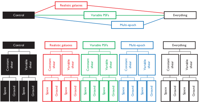
Figure 1: The GREAT3 challenge structure. This figure is taken from [15].

As described in section 2, GREAT3 focuses on three aspects of image analysis, i.e., realistic galaxies, realistically variable PSFs, and multiple different exposures. Figure 1 shows the structure of the GREAT3 challenge. The challenge consists of 5 experiments. The control experiment does not have any of these three effects. The realistic galaxy, variable PSF, and multi-epoch experiments are each dedicated tests of a single effect. The ‘everything’ experiment contains all three effects in one experiment. Each experiment has branches with constant shear and cosmologically-varying shear. For each shear configuration, simulations for a space- and ground-based telescope are prepared. Thus in total there are 20 branches.

The dominant statistical error for weak lensing shear measurement comes from the dispersion in intrinsic galaxy shapes, or shape noise. We design the challenge to cancel out the shape noise by introducing 90-degree rotated pairs in the constant shear branches and putting all the shape noise into B-mode, as for GREAT10, in the variable shear branches. This greatly increases the sensitivity of the tests for systematic biases in shear measurements.

There are 200 images per branch. Each image has a grid of 100 $\times$ 100 galaxies and represents 10 $\times$ 10 sq. degree field. Each branch of the 14 branches with variable shear and/or variable PSF has 10 distinct fields that have different underlying shear correlation functions and/or PSF variations. Each field has 20 subfields, and each subfield corresponds to a single image. Participants should estimate the shear correlation function by using the 20 subfields. On the other hand, for 6 branches with constant shear and constant PSF, shear values are different image by image. In the following subsections, we describe the details of these experiments except for the everything experiment. We then explain the actual evaluations of submissions and ranking system.

3.1 Control Experiment

In the control experiment, galaxies are generated based on a model that consists of a de Vaucouleurs bulge profile and exponential disc profile or the model of a single component Sérsic profile. The details of the model fitting is described in [11]. The distributions of the model parameters, such as size and ellipticity, are determined by the Hubble Space Telescope (HST) COSMOS survey [10, 23, 22]. These distributions are not open to participants, though the HST COSMOS data is publicly available. The distribution of signal-to-noise ratio of galaxy images is also based on the HST COSMOS survey. We set the lower limit of the signal-to-noise ratio to $S/N=20$ using the optimal definition of [4]. There are several conventions for signal-to-noise ratio. For comparison with other conventions, we find that the one-sided 99% lower limits of our signal-to-noise ratio distribution actually corresponds to $S/N$ values given by SExtractor [3] of $\simeq$10.0 (ground) and $\simeq$11.7 (space), which is comparable to the lower limit used for real weak lensing analysis.

In the control experiment, PSFs are constant across an image. PSFs are simulated in two parts: atmospheric PSF (only for ground-based simulations) and optical PSF. For atmospheric PSFs, we use the long-exposure limit atmospheric PSF model predicted by a Kolmogorov model [7]. For a single exposure we draw the size and ellipticity from their distributions estimated at the summit of Mauna Kea by the LSST Image Simulator (PhoSim [6]). For optical PSFs, we use a Zernike polynomial description of wavefront errors up to order $j=11$ in the Noll ordering [18], including trefoil and third order spherical aberration. The optical PSFs for space-based (ground-based) telescopes are obtained by fitting the model to the WFIRST-AFTA prototype model (the Dark Energy Camera early model). The PSF is given as a noiseless image for each galaxy image, so that participants should extract PSF information from the image.

3.2 Real Galaxy Experiment

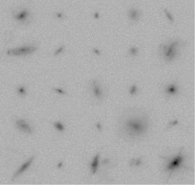
Figure 2: An example of a realistic galaxy image simulation in GREAT3. Irregular galaxy morphology can be clearly seen.

For the real galaxy experiment, we use actual galaxy images from the HST COSMOS survey. Following the procedure described in [14], the HST PSF is removed in Fourier space, the weak lensing shear and magnification are applied, and then the target PSF is applied. An example of realistic galaxy image is shown in figure 2. Note that PSFs are given in the same way as described in section 3.1.

3.3 Variable PSF Experiment

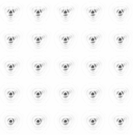
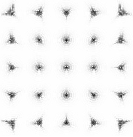
Figure 3: An example of variable, optical PSFs across the field of view. The left (right) panel shows simulations for a space-based telescope (a ground-based telescope). Both are shown on a logarithmic scale. This figure is taken from [15].

In the variable PSF experiment, PSFs vary across the field. In this experiment we aim to test PSF interpolation across the field of view, i.e., test if PSF information can be interpolated from star positions to a galaxy position. The variation is drawn from PhoSim for atmospheric PSFs and the actual optics model described above for optical PSFs. An example of optical PSFs varying across the field is shown in figure 3. Participants should extract the PSF information from star images distributed across the field of view. Since the simulated 10 $\times$ 10 sq. degree images are much larger than the field-of-view of typical telescopes, images are divided into square tiles, and a PSF model is simulated for each tile. The star images have a signal-to-noise ratio distribution with $S/N>50$ and a stellar density of about 2 arcmin^-2. The galaxy distribution is the same as for the control experiment.

3.4 Multi-epoch Experiment

In this experiment, by preparing 6 exposures with different PSFs and dithering, we aim to find an optimal way to make use of the multiple exposures, such as weighting exposures with good PSFs. The offsets between exposures are provided, so that participants do not have to infer them. The multi-epoch experiment employs the same galaxy distribution as the control experiment. Note that the signal-to-noise ratio distribution is recovered after all the exposures are combined. The distribution is not known to participants, as in the control experiment.

Data from space-based telescopes are often undersampled, i.e., not Nyquist sampled, meaning that we need either to combine multiple dithered exposures to obtain full information about PSFs, or alternatively adopt some physically motivated model that can be fit to stellar profiles to provide the lost (aliased) spatial information For space branches in the multi-epoch experiment, we prepared non-Nyquist sampled data to test this reconstruction. PSFs are given in the same way as described in section 3.1.

3.5 Evaluations and Rankings

Submissions and evaluations are done separately for each branch. Participants compete within the leader board for each branch, and are awarded points based on their best-ranked 5 branches. We award 1,000, 2,000, 4,000, 8,000, and 16,000 points for a fifth, fourth, third, second, and first-place finish, respectively. The participant with the highest point total is the winner. The first and second place winners will receive prizes.

The evaluations are done as follows. For constant shear branches, participants submit mean shear value for each of the 200 fields (a pre-submission code which calculates the mean shear based on each galaxy shape and weight is available). A linear regression is performed to provide estimates of $m_{i}$ and $c_{i}$ defined as $g^{\rm obs}_{i}-g^{\rm true}_{i}=m_{i}g^{\rm true}_{i}+c_{i}$ where $i=1,2$ denotes shear components , $g^{\rm obs}_{i}$ denotes the observed shear, and $g^{\rm true}_{i}$ denotes the true input shear. The metric for constant shear branches $Q_{c}$ is then defined by comparison of $m_{i}$ and $c_{i}$ to target values of $m_{\rm target}=2\times 10^{-3}$ and $c_{\rm target}=2\times 10^{-4}$, as required by the Euclid mission [17]. We expect $Q_{c}\simeq 1000$ ($700$) for space (ground) when a method meets the target $m_{i}$ and $c_{i}$ and smaller $Q_{c}$ for larger biases.

For variable shear branches, the evaluation involves shear correlation functions, or more specifically, aperture mass dispersions (e.g., [21]). A script for calculating aperture mass dispersions is provided, though participants can also calculate the statistics by themselves. The metric for variable shear $Q_{v}$ compares the estimates and true values, which is designed to yield $Q_{v}\simeq 1000$ $(580)$ for space (ground) when a method meets the target $m_{i}$ and $c_{i}$ and smaller $Q_{v}$ for larger biases. Higher scores for $Q_{c}$ and $Q_{v}$ are possible, due both to noise and the fact that methods may exceed target bias levels.

4 Possible Future Updates

Simulations in the GREAT3 challenge are generated by an open-source image simulation software package, GalSim, whose details will be described in an upcoming paper [20]. To test the three effects, we simplify the GREAT3 simulation images. However, for example, using GalSim, we are able to test star/galaxy separation by making images where stars and galaxies are on the same image, blending issues (overlapping galaxy images) by using non-gridded galaxies, and selection bias due to the correlation between selection criteria and PSF/galaxy shapes.

Also there are possible extensions of GalSim to make simulations more realistic. For instrument and detector specific effects, it might be useful to include charge transfer inefficiency, non-linearity, and optics and detector distortions. We will be able to test color gradients by introducing wavelength-dependent effects on galaxies and PSFs. We can test flexion measurement algorithms by adding higher-order distortions across each galaxy.

5 Conclusion

The GREAT3 challenge is an image analysis competition to test and facilitate weak lensing measurement algorithms. The challenge allows for testing bias due to complex galaxy morphology by simulated images based on real HST image, systematic uncertainties due to imperfect PSF estimation of profiles and variations across the field by simulated PSFs based on realistic atmospheric simulations and actual telescope optics designs, and optimal analysis of multiple exposures by simulated multi-epoch exposures. The challenge has started in October 2013 and will close to participants on 30 April 2014. There are several additional tests that can be done by using GalSim that is the core simulation software for GREAT3 such as star/galaxy separation and galaxy blending. There are several possible updates for GalSim such as including detector effects, wavelength-dependent effects, and flexion. The details of the challenge are described in [15].

- [1] A. Amara and A. Réfrégier, Systematic bias in cosmic shear: extending the Fisher matrix, MNRAS 391 (2008) 228
- [2] G. M. Bernstein and M. Jarvis, Shapes and Shears, Stars and Smears: Optimal Measurements for Weak Lensing, AJ 123 (2002) 583.
- [3] E. Bertin and S. Arnouts, SExtractor: Software for source extraction., A&AS 117 (1996) 393.
- [4] S. Bridle et al., Results of the GREAT08 Challenge: an image analysis competition for cosmological lensing, MNRAS 405 (2010) 2044.
- [5] S. Bridle et al., Handbook for the GREAT08 Challenge: An image analysis competition for cosmological lensing, Annals of Applied Statistics 3 (2009) 6.
- [6] A. J. Connolly et al., Simulating the LSST system, Society of Photo-Optical Instrumentation Engineers (SPIE) Conference Series, Society of Photo-Optical Instrumentation Engineers (SPIE) Conference Series 7738 (2010).
- [7] D. L. Fried, Statistics of a Geometric Representation of Wavefront Distortion, Journal of the Optical Society of America 55 (1965) 1427.
- [8] C. Heymans et al., The Shear Testing Programme - I. Weak lensing analysis of simulated ground-based observations, MNRAS 368 (2006) 1323.
- [9] T. Kitching et al., Gravitational Lensing Accuracy Testing 2010 (GREAT10) Challenge Handbook, \astroph1009.0779.
- [10] A. M. Koekemoer et al., The COSMOS Survey: Hubble Space Telescope Advanced Camera for Surveys Observations and Data Processing, ApJS 172 (2007) 196.
- [11] C. N. Lackner and J. E. Gunn, Astrophysically motivated bulge-disc decompositions of Sloan Digital Sky Survey galaxies, MNRAS 421 (2012) 2277.
- [12] R. Laureijs et al., Euclid Definition Study Report, \astroph1110.3193.
- [13] LSST Science Collaboration, LSST Science Book, Version 2.0, \astroph0912.0201.
- [14] R. Mandelbaum, C. M. Hirata, A. Leauthaud, R. J. Massey, and J. Rhodes. Precision simulation of ground-based lensing data using observations from space, MNRAS 420 (2012) 1518.
- [15] R. Mandelbaum et al., The Third Gravitational Lensing Accuracy Testing (GREAT3) Challenge Handbook, \astroph1308.4982.
- [16] R. Massey et al., The Shear Testing Programme 2: Factors affecting high-precision weak-lensing analyses, MNRAS 376 (2007) 13.
- [17] R. Massey et al., Origins of weak lensing systematics, and requirements on future instrumentation (or knowledge of instrumentation), MNRAS 429 (2013) 661.
- [18] R. J. Noll., Zernike polynomials and atmospheric turbulence, Journal of the Optical Society of America 66 (1976) 207.
- [19] A. Refregier, Shapelets - I. A method for image analysis, MNRAS 338 (2003) 35.
- [20] B. Rowe et al., in prep (2014).
- [21] P. Schneider et al., A new measure for cosmic shear, MNRAS 296 (1998) 873.
- [22] N. Scoville et al., COSMOS: Hubble Space Telescope Observations, ApJS 172 (2007) 38.
- [23] N. Scoville et al., The Cosmic Evolution Survey (COSMOS): Overview, ApJS 172 (2007) 1.
- [24] D. Spergel et al., Wide-Field InfraRed Survey Telescope-Astrophysics Focused Telescope Assets WFIRST-AFTA Final Report, \astroph1305.5422.
- [25] The Planck Collaboration, Planck 2013 results. XVI. Cosmological parameters, \astroph1303.5076.