Macroscopically deterministic, Markovian thermalization in finite quantum spin systems

Abstract

A key feature of non-equilibrium thermodynamics is the Markovian, deterministic relaxation of coarse observables such as, for example, the temperature difference between two macroscopic objects which evolves independently of almost all details of the initial state. We demonstrate that the unitary dynamics for moderately sized spin-1/2 systems may yield the same type of relaxation dynamics for a given magnetization difference. This observation might contribute to the understanding of the emergence of thermodynamics within closed quantum systems.

I introduction

Roughly 100 years after its systematic microscopic interpretation the origin of thermodynamics is still under dispute (see e.g., Uffinck (2007); Popescu et al. (2006); Beretta (2010) and references therein). It is, however, an empirical fact that macroscopic systems behave according to the laws of thermodynamics and are routinely viewed as large quantum systems. Consequently, already in the early formulations of quantum mechanics Pauli (1928); Goldstein et al. (2010); Schroedinger (1948); VanHove (1955); Tasaki (1998) the question about the relationship between quantum mechanics and thermodynamics arose and is still discussed today. A central point in the discussion is the reconciliation of unitary quantum dynamics (featuring no fixed point) with the equilibrating, rate equation-type dynamics of non-equilibrium thermodynamics (featuring a fixed point). In this debate various concepts have been introduced such as “typicality” Goldstein et al. (2010); Page (1993); Goldstein et al. (2006); Popescu et al. (2006); Gemmer and Mahler (2003); Reimann (2007), “pure state quantum statistical mechanics” Reimann (2008); Linden et al. (2009); Riera2012 “eigenstate thermalization hypothesis” Goldstein et al. (2010); Deutsch (1991); Srednicki (1994); Rigol et al. (2008); Dubey et al. (2012), “thermal environment coupling” Alicki and Lendi (1987); Caldeira and Leggett (1983); Jin et al. (2010), and many more. Recently, experiments in an optical lattice with ultra-cold atoms have been performed to study the relaxation dynamics in an interacting many-body system Trotzky et al. (2012). Also the thermalization dynamics itself, beyond the mere existence of equilibrium, has gained attention: Fokker-Planck equations for some closed finite quantum systems have been suggested Tikhonenkov et al. (2013); Ates et al. (2012); Ji et al. (2013); Niemeyer et al. (2013).

In this paper we discuss a quantum model corresponding to the archetypical thermodynamic scenario in which two (equal or similar) macroscopic bodies are prepared at, e.g., different temperatures (possibly a hot and a cold coffee mug) and then brought into contact but kept isolated from any environment. (Similar scenarios have been analyzed using quantum models in, e.g., Refs. Ponomarev et al. (2011); Zhang et al. (2012).) Experimental evidence shows that the dynamics of the temperature difference (here called $x$) is autonomous and Markovian in the sense that it may be described as

$$\dot{x}=-R(x)x,$$ (1)

where $R$ denotes the rate of change. This implies that the dynamics of the temperature difference $x$ possesses a unique, attractive fixed point, is free of memory effects and is not affected by any other variables. If the temperature difference is in some sense a statistical quantity then its variance $\sigma^{2}=\langle x^{2}\rangle-\langle x\rangle^{2}$ is expected to be small compared to the overall scale of its expectation value $\langle x\rangle$, a property referred to as macroscopic determinism. In terms of the coffee mugs this means that one may repeat the experiment several times without getting measurably different results for $x$ during its evolution.

II model and observables

The quantum model we consider is a finite, anisotropic Heisenberg spin-ladder of size $N$ described by the Hamiltonian ($\hbar=1$ throughout this paper)

$$\hat{H} =\hat{H}_{0}+\kappa\hat{V}$$

$$\hat{H}_{0} =\sum_{i=1}^{N/2-1}\sum_{\alpha=L,R}J(\hat{S}_{x}^{\alpha,i}\hat{S}_{x}^{\alpha,i+1}+\hat{S}_{y}^{\alpha,i}\hat{S}_{y}^{\alpha,i+1}+0.6\;\hat{S}_{z}^{\alpha,i}\hat{S}_{z}^{\alpha,i+1})$$

$$\hat{V} =\sum_{i=1}^{N}(\hat{S}_{x}^{L,i}\hat{S}_{x}^{R,i}+\hat{S}_{y}^{L,i}\hat{S}_{y}^{R,i}+0.6\;\hat{S}_{z}^{L,i}\hat{S}_{z}^{R,i}),$$ (2)

where $\hat{S}_{x}$, $\hat{S}_{y}$ and $\hat{S}_{z}$ denote the spin-1/2 operators, $J=1$ is the coupling strength along the beams of the ladder (labeled by $\alpha=L,R$) and $\kappa=0.2$ is the coupling strength along the rungs. The observable which is our analogon to the temperature difference mentioned in the example of the two coffee mugs is the difference of magnetization along the z-axis between the two beams which we call $\hat{x}$ throughout the paper

$$\hat{x}=\sum_{i}\hat{S}_{z}^{L,i}-\hat{S}_{z}^{R,i}.$$ (3)

Note that in the model described by Eq. (2) the total magnetization along the z-axis $\hat{S}_{z}^{total}$ of the entire system is a conserved quantity. Hence, for our analysis we choose the largest total magnetization subspace $S_{z}^{total}=0$. Within this subspace the eigenvalues of $\hat{x}$ are $X=-N/2,-N/2+2,\cdots,N/2-2,N/2$. The multiplicities are essentially binomially distributed, $X=0$ features the largest degeneracy.

In Ref. Niemeyer et al. (2013) this model has been analyzed for $N=16$ by means of exact diagonalization. Reasonable agreement of the quantum dynamics of $x$ with a Fokker-Planck equation was found numerically for a small set of initial states all of which are in a sense close to equilibrium. Furthermore the respective Fokker-Planck equation has been “derived” from an appropriate projection operator technique (up to leading order) under the assumption of equal correlation times for the transition dynamics between all $X$-subspaces. In order to investigate the claim that this finite quantum model would yield irreversible Markovian $x$-dynamics for all practical purposes, we numerically analyze the same model class in the paper at hand but for larger systems and a much wider range of initial states. We essentially find that, while indeed autonomous Markovian, deterministic $x$-dynamics emerges in general, specific predictions of the Fokker-Planck model suggested in Niemeyer et al. (2013) fail for initial states further away from equilibrium. Rather than to vanish, this failure appears to become even more pronounced for larger systems. Thus, below we present an alternative analysis based on typicality rather than on projection operator techniques which at least predicts specific equilibrium values correctly while being methodically sound.

In this paper we focus on spin systems. Relaxation in closed quantum systems is, however, not limited to spin systems, for an example of a bosonic system, see, e.g., Ref. Zhang et al. (2011).

III computational scheme and initial states

As mentioned above, in the present paper we address larger systems and a larger variety of different pure, rather than mixed, initial states. To those ends we solve the time-dependent Schrödinger equation (TDSE) numerically by means of the Chebyshev polynomial algorithm Tal-Ezer and Kosloff (1984); Leforestier et al. (1991); Iitaka et al. (1997); Dobrovitski and De Raedt (2003). This algorithm yields results that are very accurate (close to machine precision), independent of the time step used De Raedt and Michielsen (2006). Conserved quantities such as the total energy and magnetization are constant to almost machine precision (about 14 digits in our calculations). Computer memory severely limits the sizes of the quantum spin systems which can be simulated. To represent the state $\left|\Psi(t)\right\rangle$ of $N$ spin-$1/2$ particles on a digital computer, we need a least $2^{N+4}$ bytes. In practice, we need several of such vectors, memory for communication buffers, local variables and the code itself. For example, for $N=32$ we need about 320 GB of memory. Although the CPU time required to solve the TDSE also increases exponentially with the number of spins, this increase can be compensated for by distributing the calculations over many processors. For a $N=32$ system, solving the TDSE upto $t=150$ using 65536 CPUs takes about 6 hours on the Jülich IBM BlueGene/Q. Details of the massively parallel simulation code are given in Ref. De Raedt et al. (2007).

To account for the initial state independence as described in the introduction, we draw pure states essentially at random, only tailored to feature probability distributions with respect to $x$ and energy that are narrow compared to the overall range of possible values for the respective observables. From the numerics it turns out that the narrow energy distribution is crucial for the expected dynamics to emerge. If the initial states are drawn from a larger energy window the equilibrium variances $\sigma^{2}$ exhibit a strong dependence on the initial state which is obviously in conflict with the concept of a thermodynamic equilibrium. Our understanding of this phenomenon is not conclusive yet, we however expect that its occurrence strongly depends on the degree to which the eigenstate thermalization hypothesis is fulfilled. We intend to discuss this thoroughly in a forthcoming paper Steingeweg et al. (2013). The initial states $|\omega_{X}\rangle$ are constructed as follows. We begin with the states $|\Psi\rangle=\sum_{j=1}^{2^{N}}c_{j}\left|j\right\rangle$, where the set of states $\left\{\left|j\right\rangle\right\}$ denotes the complete basis set of states in the spin-up – spin-down representation and the coefficients $c_{j}$ are obtained by generating uniform independent random numbers in the interval $[-1,1]$ and rescaling them such that $\sum_{j=1}^{2^{N}}|c_{j}|^{2}=1$. We then project the initial state to the “$S_{z}^{total}=0$-and-specific-$X$-subspace” and in order to narrow down the energy distribution (in this case around $\langle\hat{H}\rangle=0$) we eventually apply a pertinent exponential

$$|\omega_{X}\rangle=Ce^{-\alpha\hat{H}^{2}}\hat{P}_{x}\hat{P}(S_{z}=0)|\Psi\rangle,$$ (4)

with $\hat{P}_{x}$ being the projector onto a subspace featuring a certain eigenvalue of $\hat{x}$, $\hat{P}(S_{z}=0)$ being the projector on the $S_{z}^{total}=0$ subspace and $\alpha$ denoting a constant chosen such that the variance of the energy $\sigma_{H}^{2}$ for the initial states $\omega$ is small ($\sigma_{H}=0.37$ is used throughout this paper for the reasons explained above). $C$ is just a normalization constant. To compute $e^{-\alpha\hat{H}^{2}}|\phi\rangle$ the same Chebyshev polynomial algorithm is used as for the time evolution. Of course, using this algorithm the energy window can also be located at positions other than $\langle\hat{H}\rangle=0$. In this paper, however, we choose $\langle\hat{H}\rangle=0$ since it appears to be the most promising choice for the emergence of thermodynamical behavior: In this model $\langle\hat{H}\rangle=0$ is in the center of the full energy spectrum and features the largest density of states. Furthermore $\langle\hat{H}\rangle=0$ would also be the energy expectation value of a hypothetical Gibbs equilibrium state with infinite temperature. So in this respect the choice $\langle\hat{H}\rangle=0$ corresponds to a high temperature limit. The case of $\langle\hat{H}\rangle$ closer to the ground state energy, i.e., lower temperatures is left as an interesting subject for further investigation.

IV discussion of the dynamics

As a first result we find that initial states with the same $\langle\hat{x}(0)\rangle$ and $\alpha$ but generated from different random $|\Psi\rangle$ show approximately the same dynamics of, e.g., mean $\langle\hat{x}(t)\rangle$ and variance $\sigma^{2}(t)=\langle\hat{x}(t)^{2}\rangle-\langle\hat{x}(t)\rangle^{2}$. This was also found and discussed in Ref. Niemeyer et al. (2013) for $N=16$. However, for $N=32$ this becomes so pronounced that the respective graphs cannot be discriminated by the naked eye. Therefore, in what follows we only present results for initial states generated from one random $|\Psi\rangle$. This finding may be viewed as a manifestation of the concept of dynamical typicality Bartsch and Gemmer (2009) and is in accord with results presented in Refs. Hams and De Raedt (2000); Elsayed and Fine (2013).

Next we turn towards an overall picture of the $x$-dynamics in this model. Fig. 1 shows the dynamics of the probabilities $P_{x}=\langle\hat{P}_{x}\rangle$ for two initial states with $\langle\hat{x}(0)\rangle=8$ and $\langle\hat{x}(0)\rangle=-6$, respectively, for $N=32$.

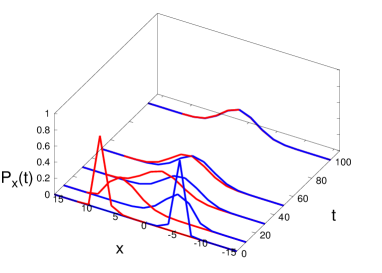
Figure 1: (color online). Dynamics of the probability distribution ${P}_{x}(t)$ for spin-ladders of size $N=32$ for two different essentially random initial states with $\langle\hat{x}(0)\rangle=8$ (red line) and $\langle\hat{x}(0)\rangle=-6$ (blue line). The two probability distributions hardly overlap at $t=0$ and almost coincide at later times.

Obviously the unitary dynamics yields after some time essentially constant probabilities $P_{x}(t)$ which coincide for both initial states while they hardly overlap at $t=0$. This can be interpreted as a strong indication for thermodynamic behaviour in this spin system. To analyze this further we focus on the dynamics of the magnetization difference $\langle\hat{x}(t)\rangle$ and its variance $\sigma^{2}(t)=\langle\hat{x}(t)^{2}\rangle-\langle\hat{x}(t)\rangle^{2}$.

In Ref. Niemeyer et al. (2013) it has been argued that the $x$ dynamics of the model could be captured by a Markovian master equation derived from a simple stochastic spin-flip model. The transition rates between neighboring $x$-subspaces read

$$R_{(X\rightarrow X\pm 2)}=\frac{\gamma\kappa^{2}N}{2}\left(\frac{1}{2}\mp\frac{X}{N}\right)^{2},$$ (5)

where $\gamma$ denotes an overall time constant.

Master equations with rates (5) necessarily yield autonomous dynamics. The $x$-dynamics as resulting from the Schrödinger equation and from the above master equation are compared to each other for two different initial states for $N=16$, see Fig. 2. While the agreement for the initial state close to equilibrium is quite good ($\langle\hat{x}(0)\rangle=2$) the stochastic model (5) fails to predict the dynamics for states starting far from equilibrium ($\langle\hat{x}(0)\rangle=6$). In Ref. Niemeyer et al. (2013) it was suggested that this failure may vanish for larger system sizes. With the work at hand we are able to address such larger system sizes. Data equivalent to Fig. 2 but now for $N=32$ is given in Fig. 3. Obviously the agreement for initial states close to equilibrium ($\langle\hat{x}(0)\rangle=2$) becomes even better but the failure for substantially off-equilibrium initial states ($\langle\hat{x}(0)\rangle=12$) remains. Since the agreement of (5) with the true quantum dynamics does not improve for off-equilibrium states with increasing system size the crucial question remains whether the true quantum dynamics may nevertheless be considered in accord with macroscopically deterministic, irreversible, Markovian behavior of $x(t)$ for larger $N$.

In order to address this question we compute $\langle\hat{x}(t)\rangle$ for various $\langle\hat{x}(0)\rangle$ for $N=32$ and display the result in Fig. 4. The curves are shifted in time such that the squares of the deviations of the curves from one another are minimized. If the dynamics was fully autonomous and Markovian, the curves would lie exactly on top of each other. Apparently, this is to good accuracy the case for all initial states, regardless of the failure of (5). In Fig. 4 the variances $\sigma^{2}(t)$ are displayed for the same initial states. Although the master equation based on (5) does not describe the dynamics correctly, all variances appear to converge to the same value. This finding is also in accord with Markovian irreversible behavior.

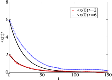
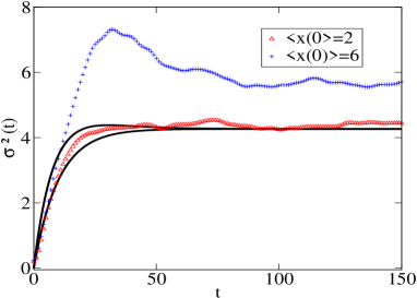
Figure 2: (color online). (a) Expectation values $\langle\hat{x}(t)\rangle$ of the magnetization difference for $N=16$ for two states, one starting close to equilibrium $\langle\hat{x}(0)\rangle=2$ and the other far from equilibrium $\langle\hat{x}(0)\rangle=6$. Solid lines represent the corresponding data as calculated from the stochastic model suggested in Ref. Niemeyer et al. (2013). Close to equilibrium the agreement is good while more off-equilibrium it is not. (b) Equivalent data and style of presentation as in (a) but for the variances $\sigma^{2}(t)$.

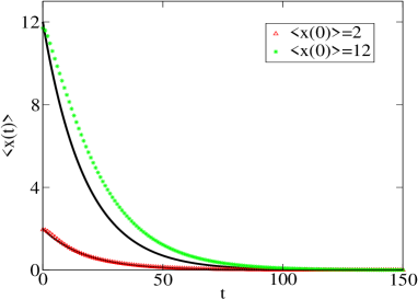
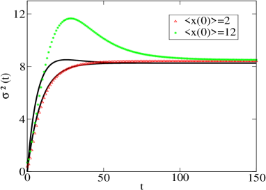
Figure 3: (color online). (a, b) Equivalent data and style of presentation as in Fig. 2 but for $N=32$. ( $\langle\hat{x}(0)\rangle=12$ here represents off-equilibrium ). While the agreement close to equilibrium is better than for $N=16$, for off-equilibrium initial states this appears not to be the case.

How can this “irreversible” tendency of the variances corresponding to so many pure, different initial states towards one constant “equilibrium” value be explained although the description in terms of the master equation defined by (5) fails? An explanation may be provided by the concept of typicality. The equilibrium value coincides with the typical variance $\sigma^{2}_{typical}$, see Fig. 4. The latter is the “generic” variance of a random initial state which is unrestricted with respect to $\langle\hat{x}\rangle$, i.e. $|\omega^{\prime}\rangle=e^{-\alpha\hat{H}^{2}}|\Psi\rangle$ (cf. also Sugiura and Shimizu (2012)): Within the addressed energy shell there are certainly states featuring variances ranging from $\approx 0.5$ to $\approx N^{2}/16$. However, as shown in the context of typicality, states featuring a certain variance $\sigma^{2}_{typical}$ are by far the most frequent ones, with respect to the unitary invariant measure Bartsch and Gemmer (2009). Therefore they are sometimes called “typical states”. While all considered initial states start in a very tiny region of Hilbert space formed by “non-typical” states, some states venture out into the extremely large region formed by the typical states, while other initial states do not such as, e.g., the initial state coresponding to $\langle\hat{x}(0)\rangle=6$ in Fig. 2. Its variance $\sigma^{2}(t)$ remains significantly above the typical variance. However, the corresponding data for $N=32$ as displayed in Fig. 4 indicate that the relative amount of states that does reach the typical region essentially increases up to $100\%$ rather quickly with system size.

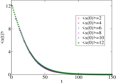
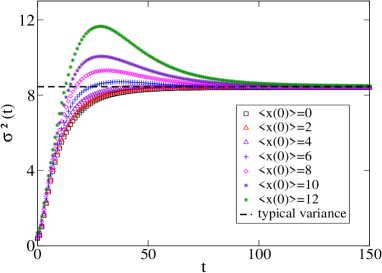
Figure 4: (color online). (a) Expectation values $\langle\hat{x}(t)\rangle$ of the magnetization difference for $N=32$ and initial states featuring different $\langle\hat{x}(0)\rangle$. Graphs are shifted in time for optimal agreement. (b) Variances $\sigma^{2}$ of the magnetization difference for $N=32$ and initial states featuring different $\langle\hat{x}(0)\rangle$ (unlike (a), no time shift is applied). The dashed line indicates the typical variance (see text).

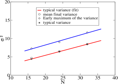
Figure 5: (color online). Scaling of three quantities concerning variances with system size $N$: ($\circ$), average over all addressed final variances as displayed, e.g., in Figs. 2, 4, ($\ast$) typical variances (see text), ($\diamond$) largest early maxima as visible, e.g., in Figs. 2, 4. Solid lines are linear fits to the typical variances (red) and the early maxima (blue). The coincidence of the mean variances with the typical variances is very good for larger $N$. All quantities appear to scale linearly with system size, the early maxima are above the mean final variances by a constant shift of $\approx 3$

Next we address the question how the final variances and their maxima (as visible, e.g., in Fig. 4) scale with the system size. Since the predictability of the quantum dynamics by (5) does not fully hold this scaling is crucial for the claim that this model shows irreversible, macroscopically deterministic behaviour. In Fig. 5 the mean of the final variances averaged over all discussed initial states, the typical variances and the largest maxima of the variances are shown for $N=16,24,32$. These maxima occur before the eventual values are reached and are most pronounced for the respective most “off-equilibrium” initial states, i.e., the states with the largest $|\langle\hat{x}(0)\rangle|$, cf. Figs.  2, 4. These early, most pronounced maxima appear to be above the final variances by a finite shift of $\approx 3$ for all system sizes as may be inferred from Fig. 5. Figure 5 also indicates that, at least for $N=24,32$, the final variances agree very well with the typical variances as already mentioned above. It is also clearly seen that all displayed quantities scale linearly with the system size and feature the same slope.

The above findings may be summarized and interpreted as follows: Figure 4 strongly indicates that the expectation value of the magnetization difference $x$ shows autonomous and Markovian dynamics. Figure 4 indicates that its variances may go through early maxima but eventually tightly cluster around the typical variance. Figure 5 indicates that throughout the dynamics the standard deviations $\sigma$ of the magnetization difference essentially scale as $\sigma\propto\sqrt{N}$. Since the maximum $\langle\hat{x}\rangle$ scales linearily with the system size as $N$ this means that the standard deviation will vanish compared to the overall scale of the expectation values with increasing system size. Therefore the specifications for thermodynamic behaviour given in the introduction (autonomous and Markovian dynamics for the expectation value and negligible variances on the scale defined by the expectation values) are met for this system.

V stochastic dynamics beyond macroscopic determinism

Considering the correspondence with macroscopic thermodynamic properties the question comes to mind whether the dynamics of $\langle\hat{x}\rangle$ and $\sigma^{2}$ can be effectively described by a (discrete) Markov chain on the magnetization difference subspaces, regardless of the failure of the model suggested in Ref. Niemeyer et al. (2013) for larger $|X|$. As already pointed out in the above discussion of Figs. 2, 3 this Markov chain should be similar to the model defined by (5) close to equilibrium but should significantly deviate from the latter for transitions between subspaces with larger $|X|$. In a sense, which is described in more detail below, this Markov chain can be expected to be comparable to a Fokker-Planck equation. Moreover, due to the autonomy of the dynamics of $\langle\hat{x}(t)\rangle$ this Markov chain must correspond to a Fokker-Planck equation with a drift or force term, the curvature of which is negligible on the scale of $\sigma$. The existence of such a Markov chain would imply the validity of what Van Kampen called the “assumption of repeated randomness” van Kampen (1962); Uffinck (2007) for this specific system (It may be worth noting here that Van Kampen and others built their explanation of the second law on this assumption.). Thus, in order to check whether such a Markov chain exists and to find its concrete form we compute the finite transition probabilities $w_{XY}(\tau)$ between all subspaces according to :

$$w_{XY}(\tau):=|\hat{P}_{X}e^{-i\tau\hat{H}}|\omega_{Y}\rangle|^{2}.$$ (6)

If such a description applies, the dynamics of the probabilities should be given by $P_{X}(t)$ :

$$\vec{P}(n\tau)=W(\tau)^{n}\vec{P}(0),$$ (7)

where $\vec{P}(t)$ represents the entity of all $\{P_{X}(t)\}$ as a vector, and $W(\tau)$ is the transition matrix formed by all $\{w_{XY}(\tau)\}$. From $\vec{P}(t)$ the mean and variance may be computed as

$$<x(t)>=\vec{X}\cdot\vec{P}(t),\quad\sigma^{2}=\vec{X^{2}}\cdot\vec{P}(t)-(\vec{X}\cdot\vec{P}(t))^{2},$$ (8)

where $\vec{X}$ is the vector formed by all $\{X\}$ and $\vec{X^{2}}$ the vector formed by all $\{X^{2}\}$. In Fig. 6 we compare the dynamics of mean and variance as resulting from the unitary evolution to the dynamics as resulting from (6, 7) for $\tau=15$ (this choice is not imperative, however for $\tau$ on the timescale of the correlation time the agreement becomes worse).

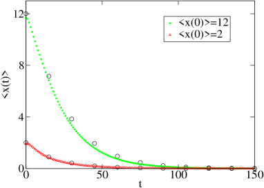
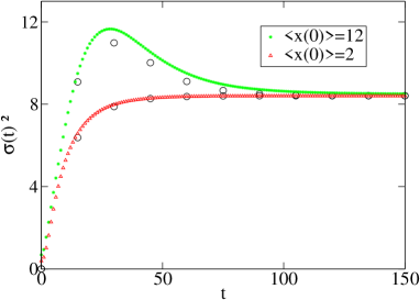
Figure 6: (color online). (a) Expectation values $\langle\hat{x}(t)\rangle$ of the magnetization difference for $N=32$ for two states, one starting close to equilibrium $\langle\hat{x}(0)\rangle=2$ and the other far from equilibrium $\langle\hat{x}(0)\rangle=12$. Circles ($\circ$) represent the corresponding data as calculated from the Markov chain specified by (6). (b) Equivalent data and style of presentation as in (a) but for the variances $\sigma^{2}(t)$. This is to be compared with Fig. 3. Obviously the agreement of the quantum dynamics with data from Markov chain is better than with results from the spin-flip model suggested in Ref. Niemeyer et al. (2013).

Obviously there is reasonable agreement even for states starting far from equilibrium. This indicates that a Markov chain based on $W(\tau)$ may indeed essentially capture the dynamics of the closed quantum system. In order to compare the Markov chain defined by (7) to the master equation defined by (5) we first compute a matrix of finite transition probabilities $u_{XY}(\tau)$ as resulting from (5). This is conveniently done numerically. Since we intend to compare with $w_{XY}(\tau=15)$ of course we compute also $u_{XY}(\tau=15)$. In order to be able to compare $w_{XY}(\tau=15),u_{XY}(\tau=15)$ in a meaningful way we assign to both transition matrices a “force” $f(X)$ and a “diffusion coefficient” $D(X)$ in the following way: We compute the change of the mean $<x(t)>$ during time $t=15$ given that one started with $<x(0)>=X$, we call that $f(X)$. Furthermore we compute the increase of the variance $\sigma^{2}(t)$ during time $t=15$ given that one started with $<x(0)>=X,\sigma^{2}(0)\approx 0$, we call that $D(X)$.

The results for the forces and the diffusion coefficients are displayed in Fig. 7

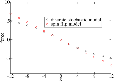
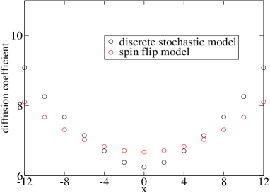
Figure 7: (color online). (a) Quantity corresponding to a force term in a Fokker-Planck equation, calculated from the spin-flip model defined by (5) (red circles) and the discrete stochastic model (6) (black circles). While the force for the spin flip model is almost strictly linear, the force for the discrete stochastic model deviates from that in the off-equilibrium regime. However, the curvature is low on the scale of $\sigma$ ($\approx 3$). (b) Equivalent data and display style as in (a) but for a quantity corresponding to the diffusion term in a Fokker-Planck equation. The diffusion coefficient for both models deviate slightly from each other.

Obviously there is a good agreement for the force and reasonable agreement for the diffusion coefficient as calculated from the Markov chain (6) and the spin-flip model (5) close to equilibrium ($X=0$). However there are also significant differences in the off-equilibrium regime. Based on the numerics at hand we did not find any tendency of these differences to vanish in the limit of larger systems.

VI summary, conclusion and outlook

In this paper we have demonstrated that a finite quantum system may show thermodynamic behaviour in the sense of macroscopically deterministic, autonomous, Markovian relaxation of an observable for a very large class of pure initial states. While this behavior gets more pronounced under upscaling it is already visible for a system comprising $32$ spins. Although being in a well-defined sense Markovian, the above relaxation dynamics is not in full accord with the naive model presented in Ref. Niemeyer et al. (2013). However, this finding nonetheless supports the view of irreversible, stochastic dynamics of selected observables emerging directly from quantum mechanics. Of course this emergence of thermodynamical relaxation directly leads to the quest for a sensible definition of entropy in this context. Since (regardless of the failure of the Fokker-Planck based model in Ref. Niemeyer et al. (2013) the dynamics is found to be in accord with a specific Markov chain) such a notion could be provided by the concept of stochastic thermodynamics as described, e.g., in Refs Sekimoto (1998); Lebowitz and Spohn (1999); Seifert (2005); Esposito (2010). (For a comprehensive introduction see also Seifert (2012).) This concept has already been applied to Markovian, Esposito and Mukamel (2006) and non-Markovian Kawamoto and Hatano (2011) open quantum systems. The model presented in the paper at hand could provide an access to a systematic application of stochastic thermodynamics to closed quantum systems.

This work is supported in part by NCF, The Netherlands (HDR). The authors gratefully acknowledge the computing time granted by the JARA-HPC Vergabegremium and provided on the JARA-HPC Partition part of the supercomputer JUQUEEN at Forschungszentrum Jülich.

References

- Uffinck (2007) J. Uffinck, Compendium to the foundation of statistical physics, edited by J. Butterfield and J. Earman, Handbook for the Philosophy of Physics (Elsevier, Amsterdam, 2007) pp. 924–1074.
- Popescu et al. (2006) S. Popescu, A. Short, and A. Winter, Nature Physics 2, 754 (2006).
- Beretta (2010) G. P. Beretta, J. Phys.: Conf. Ser. 237, 012004 (2010).
- Pauli (1928) W. Pauli, Festschrift zum 60. Geburtstage A. Sommerfelds (Hirzel, 1928) p. 30.
- Goldstein et al. (2010) S. Goldstein, J. L. Lebowitz, R. Tumulka, and N. Zanghi, Eur. Phys. J. H 35, 173 (2010).
- Schroedinger (1948) E. Schroedinger, Statistical Thermodynamics, A Course of Seminar Lectures (Cambridge University Press, 1948).
- VanHove (1955) L. VanHove, Physica 21, 517 (1955).
- Tasaki (1998) H. Tasaki, Phys. Rev. Lett. 80, 1373 (1998).
- Page (1993) D.N Page, Phys. Rev. Lett. 71, 1291 (1993).
- Goldstein et al. (2006) S. Goldstein, J.L Lebowitz, R. Tumulka, and N. Zanghi, Phys. Rev. Lett. 96, 050403 (2006).
- Gemmer and Mahler (2003) J. Gemmer and G. Mahler, Eur. Phys. J. B 31, 249 (2003).
- Reimann (2007) P. Reimann, Phys. Rev. Lett. 99, 160404 (2007).
- Reimann (2008) P. Reimann, Phys. Rev. Lett. 101, 190403 (2008).
- Linden et al. (2009) N. Linden, S. Popescu, A. J. Short, and A. Winter, Phys. Rev. E 79, 061103 (2009).
- Riera et al. (2012) A. Riera, C. Gogolin, and J. Eisert, Phys. Rev. Lett. 108, 080402 (2012).
- Deutsch (1991) J. M. Deutsch, Phys. Rev. A 43, 2046 (1991).
- Srednicki (1994) M. Srednicki, Phys. Rev. E 50, 888 (1994).
- Rigol et al. (2008) M. Rigol, V. Dunjiko, and M. Olshanii, Nature 452, 854 (2008).
- Dubey et al. (2012) S. Dubey, L. Silvestri, J. Finn, S. Vinjanampathy, and K. Jacobs, Phys. Rev. E 85, 011141 (2012).
- Alicki and Lendi (1987) R. Alicki and K. Lendi, Quantum dynamical semigroups and applications, Lecture Notes in Physics, Vol. 286 (Springer, 1987).
- Caldeira and Leggett (1983) A. O. Caldeira and A. J. Leggett, Physica A 121, 587 (1983).
- Jin et al. (2010) F. Jin, H. De Raedt, S. Yuan, M. I. Katsnelson, S. Miyashita, and K. Michielsen, J. Phys. Soc. Jpn. 79, 124005 (2010).
- Trotzky et al. (2012) S. Trotzky, Y. Chen, A. Flesch, I. McCulloch, U. Schollwock, J. Eisert, and I. Bloch, Nature Phys. 8, 325 (2012).
- Tikhonenkov et al. (2013) I. Tikhonenkov, A. Vardi, J. R. Anglin, and D. Cohen, Phys. Rev. Lett. 110, 050401 (2013).
- Ates et al. (2012) C. Ates, J. P. Garrahan, and I. Lesanovsky, Phys. Rev. Lett. 108, 110603 (2012).
- Ji et al. (2013) S. Ji, C. Ates, J. P. Garrahan, and I. Lesanovsky, J. Stat. Mech. 2013, P02005 (2013).
- Niemeyer et al. (2013) H. Niemeyer, D. Schmidtke, and J. Gemmer, Eur. Phys. Lett. 101, 10010 (2013).
- Ponomarev et al. (2011) A. V. Ponomarev, S. Denisov, and P. Hanggi, Phys. Rev. Lett. 106, 010405 (2011).
- Zhang et al. (2012) J.M Zhang, C. Shen, and W.M Liu, Phys. Rev. A 85, 013637 (2012).
- Zhang et al. (2011) J.M Zhang, C. Shen, and W.M Liu, Phys. Rev. A 83, 063622 (2011).
- Tal-Ezer and Kosloff (1984) H. Tal-Ezer and R. Kosloff, J. Chem. Phys. 81, 3967 (1984).
- Leforestier et al. (1991) C. Leforestier, R. H. Bisseling, C. Cerjan, M. D. Feit, R. Friesner, A. Guldberg, A. Hammerich, G. Jolicard, W. Karrlein, H.-D. Meyer, N. Lipkin, O. Roncero, and R. Kosloff, J. Comp. Phys. 94, 59 (1991).
- Iitaka et al. (1997) T. Iitaka, S. Nomura, H. Hirayama, X. Zhao, Y. Aoyagi, and T. Sugano, Phys. Rev. E 56, 1222 (1997).
- Dobrovitski and De Raedt (2003) V. V. Dobrovitski and H.A De Raedt, Phys. Rev. E 67, 056702 (2003).
- De Raedt and Michielsen (2006) H. De Raedt and K. Michielsen, in Handbook of Theoretical and Computational Nanotechnology, edited by M. Rieth and W. Schommers (American Scientific Publishers, Los Angeles, 2006) pp. 2 – 48.
- De Raedt et al. (2007) K. De Raedt, K. Michielsen, H. De Raedt, B. Trieu, G. Arnold, M. Richter, T. Lippert, H. Watanabe, and N. Ito, Comp. Phys. Comm. 176, 121 (2007).
- Steingeweg et al. (2013) R. Steingeweg, H. Niemeyer, C. Gogolin, and J. Gemmer, arXiv: 1311.0169 (2013).
- Bartsch and Gemmer (2009) C. Bartsch and J. Gemmer, Phys. Rev. Lett. 102, 110403 (2009).
- Hams and De Raedt (2000) A. Hams and H. De Raedt, Phys. Rev. E 62, 4365 (2000).
- Elsayed and Fine (2013) T. A. Elsayed and B.V. Fine, Phys. Rev. Lett. 110, 070404 (2013).
- Sugiura and Shimizu (2012) S. Sugiura and A. Shimizu, Phys. Rev. Lett. 108, 240401 (2012).
- van Kampen (1962) N. van Kampen, Fundamental Problems in the Statistical mechanics of irreversible processes, edited by E. Cohen, Fundamental Problems in statistical mechanics (North Holland, Amsterdam, 1962) pp. 173–202.
- Sekimoto (1998) K. Sekimoto, Prog. Theor. Phys. Suppl. 130, 17 (1998).
- Lebowitz and Spohn (1999) J. Lebowitz and H. Spohn, J. Stat. Phys. 95, 333 (1999).
- Seifert (2005) U. Seifert, Phys. Rev. Lett. 95, 040602 (2005).
- Esposito (2010) M. Esposito and C. Van den Broeck, Phys. Rev. Lett. 104, 090601 (2010).
- Seifert (2012) U. Seifert, Rep. Prog. Phys. 75, 126001 (2012).
- Esposito and Mukamel (2006) M. Esposito and S. Mukamel, Phys. Rev. E 73, 046129 (2006).
- Kawamoto and Hatano (2011) T. Kawamoto and N. Hatano, Phys. Rev. E 84, 031116 (2011).