Non-linear eigenvalue problems arising from growth maximization of positive linear dynamical systems

Non-linear eigenvalue problems arising from growth maximization of positive linear dynamical systems

Abstract

We study a growth maximization problem for a continuous time positive linear system with switches. This is motivated by a problem of mathematical biology (modeling growth-fragmentation processes and the PMCA protocol). We show that the growth rate is determined by the non-linear eigenvalue of a max-plus analogue of the Ruelle-Perron-Frobenius operator, or equivalently, by the ergodic constant of a Hamilton-Jacobi (HJ) partial differential equation, the solutions or subsolutions of which yield Barabanov and extremal norms, respectively. We exploit contraction properties of order preserving flows, with respect to Hilbert’s projective metric, to show that the non-linear eigenvector of the operator, or the “weak KAM” solution of the HJ equation, does exist. Low dimensional examples are presented, showing that the optimal control can lead to a limit cycle.

I Introduction

We investigate in this note the optimal control of time continuous positive linear dynamical systems in infinite horizon. We wish to compute the maximal growth rate that can be obtained from infinitesimal combinations of a set of nonnegative matrices.

More precisely, we consider a compact set $\mathcal{M}\subset\mathcal{M}_{n}({\mathbb{R}})$ of irreducible Metzler matrices. That is to say, we assume that for all $m\in\mathcal{M}$ and for all $i\neq j$, $m_{ij}\geq 0$. In addition for every partition of indices $\{1\dots n\}={I\mathbin{\mathchoice{\leavevmode\vtop{\halign{\hfil$\m@th\displaystyle#$\hfil\cr\cup\cr\cdot\crcr}}}{\leavevmode\vtop{\halign{\hfil$\m@th\textstyle#$\hfil\cr\cup\cr\cdot\crcr}}}{\leavevmode\vtop{\halign{\hfil$\m@th\scriptstyle#$\hfil\cr\cup\cr\cdot\crcr}}}{\leavevmode\vtop{\halign{\hfil$\m@th\scriptscriptstyle#$\hfil\cr\cup\cr\cdot\crcr}}}}J}$ one can pick $i\in I$ and $j\in J$ such that $m_{ij}>0$. A direct consequence of compactness is uniform irreducibility: there exists a constant $\nu>0$ such that for all $m\in\mathcal{M}$, and every partition of indices one can pick $i\in I$ and $j\in J$ such that $m_{ij}\geq\nu$.

Let $K$ be the nonnegative orthant in ${\mathbb{R}}^{n}$, $K_{+}$ the positive orthant, and $K_{0}=K\setminus\{0\}$. For $t>0$, $x\in K$ and a measurable control function $M:[0,t]\to\mathcal{M}$, we define $x_{M}\in W^{1,\infty}([0,t],{\mathbb{R}}^{n})$ as the solution of the following linear problem with control $M$:

$$\begin{cases}\dot{x}_{M}(s)=M(s)x_{M}(s),\\ x_{M}(0)=x\,.\end{cases}$$ (1)

We also denote $x_{M}(s)=R(s,M)x$, where $R$ is the resolvent. Finally we denote in short $L^{\infty}(0,t)$ the set of measurable (bounded by assumption) control functions $M:[0,t]\to\mathcal{M}$. We are interested in control functions maximizing the growth rate

$$\limsup_{t\to\infty}\frac{1}{t}\log\|x_{M}(t)\|\enspace.$$ (2)

We assume w.l.o.g. that $\mathcal{M}$ is convex. The results presented here are still valid for nonconvex sets $\mathcal{M}$, provided the controls are replaced by relaxed controls which take values in the closed convex hull $\overline{\mathrm{co}}\,(\mathcal{M})$.

For a constant control $M(s)\equiv m$ we have $R(t,m)=e^{tm}$. It is an immediate consequence of the Perron-Frobenius theorem that, being $\phi_{m}\in K_{+}$ a left Perron-Frobenius (PF) eigenvector of $m$, the linear function $\overline{v}(x)=\left\langle\phi_{m},x\right\rangle$ satisfies the following identity,

$$(\forall t\in\mathbb{R}_{+})\;(\forall x\in K)\quad e^{\lambda(m)t}\overline{v}(x)=\overline{v}(x_{m}(t))\,,$$

where $\lambda(m)\in\mathbb{R}$ is the dominant eigenvalue of $m$. The following result can be thought of as a non-linear extension of the Perron-Frobenius theorem.

Theorem 1

Under previous assumptions there exist a real $\lambda(\mathcal{M})$ and a function $\overline{v}:K\to{\mathbb{R}}_{+}$, homogeneous of degree 1, positive on $K_{0}$, globally Lipschitz continuous, which satisfy the following identity

$$(\forall t\in\mathbb{R}_{+})\;(\forall x\in K)\quad e^{{\lambda(\mathcal{M})}t}\overline{v}(x)=\sup_{M\in L^{\infty}(0,t)}\overline{v}(x_{M}(t))\,,$$ (3)

The scalar $\lambda(\mathcal{M})$ is unique as soon as $\overline{v}$ belongs to the class of homogeneous functions of degree 1 which are locally bounded on $K$, and it determines the optimal growth rate (2). Moreover, $\overline{u}=\log\overline{v}$ is characterized as a viscosity solution of an ergodic Hamilton-Jacobi PDE:

$$-\lambda(\mathcal{M})+H(D_{y}\overline{u}(y),y)=0\,,{\quad y\in\mathcal{S}}\,,$$ (4)

where $\mathcal{S}$ is the standard simplex.

The Hamiltonian $H$ will be given in Section II.

Corollary 2 (Ergodicity)

Let $v_{0}:K\to{\mathbb{R}}_{+}$ be a continuous function, homogeneous of degree 1, positive on $K_{0}$. Define $v(t,x)=\sup_{M\in L^{\infty}(0,t)}v_{0}(x_{M}(t))$. Then we have the following ergodicity result,

$$(\forall x\in{K_{0}})\quad\lim_{t\to+\infty}\frac{1}{t}\log(v(t,x))=\lambda(\mathcal{M})\,.\$$

Moreover the convergence is locally uniform on $K_{0}$.

Theorem 1 is closely related to results belonging to the theory of stability of linear inclusions. There, matrices are not necessarily assumed to be Metzler matrices. The non-linear eigenvalue $\lambda({\mathcal{M}})$ coincides with the joint spectral radius [32]. In his seminal paper [4], Barabanov proved the existence of extremal norms in ${\mathbb{R}}^{n}$ which saturates (3), under a different irreducibility condition. Later the same author investigated the behaviour of extremal trajectories in the three-dimensional case $n=3$, first when $\mathcal{M}$ has the specific structure of a segment with a rank one matrice for direction [5], secondly under a uniqueness condition for extremal trajectories verifying the Pontryagin Maximum Principle (PMP) [6] (see also the recent improvement by Gaye et al [22]). We also refer to [35] for an alternative proof of the existence of Barabanov extremal norms, and to the work of Chitour, Mason and Sigalotti [13] for the analysis of situations in which there are obstructions to the existence of such norms.

Several authors have analyzed specially the stability of positive linear systems. Very recently, Mason and Wirth [28] have established the existence of an extremal norm, that is, a viscosity subsolution of the spectral problem (3) (the equality relation being replaced by $\geq$), corresponding to a critical subsolution of the ergodic Hamilton-Jacobi equation. They use an irreducibility condition which is milder than our, but which does not guarantee the existence of a viscosity solution. Conditions for the existence of subsolutions are typically less restrictive. It is an interesting issue to see whether the assumptions of Theorem 1 could be relaxed.

We emphasize that we take advantage of an illuminating connection between problem (3) and the weak KAM theory in Lagrangian dynamics [20]. In particular long-time dynamics of optimal trajectories appear to be encoded in the so-called Aubry sets. Such eigenproblems have been widely studied in ergodic control, and also by dynamicians in the setting of the weak KAM theory, where the eigenfunction is known as a weak KAM solution. However, basic existence results for eigenvectors rely on controllability conditions which are not satisfied in our setting.

We exploit tools from the theory of Hamilton-Jacobi PDE to prove Theorem 1, combined with techniques from Perron-Frobenius theory. In particular, we use the Birkhoff-Hopf theorem in a crucial way. The latter states that a linear map leaving invariant the interior of a closed, convex and pointed cone is a strict contraction in Hilbert’s projective metric. The contraction of the controlled flow turns out to entail the existence of the eigenvector. We note that tools from Lagrangian dynamics (Mather sets) have been recently applied by Morris to study joint spectral radii [30]. This deserves to be further studied in the present setting.

The same type of equations has been studied in the context of infinite dimensional max-plus spectral theory. In particular, the existence of continuous eigenfunctions for max-plus operators with a continuous kernel is established in [24]. More general conditions, exploiting quasi-compactness techniques, can be found in [26]. It would be interesting to see whether such techniques to the present problems.

A natural question that arises in the literature is whether the knowledge of $\{\lambda(m)\}_{m\in\mathcal{M}}$, say $(\forall m\in\mathcal{M})\;\lambda(m)<0$ guarantees the stability of the differential inclusion (1). A positive answer has been given in [23] in dimension $n=2$. A negative answer has been given in (possibly) high dimension in the same work. Soon after, Fainshil et al give a counter-example in dimension $n=3$ [18]. It is a pair of matrices such that every convex combination has a negative spectral radius but the associated joint spectral radius is positive.

We address similar questions in the present note, namely whether $\lambda(\mathcal{M})=\max_{m}\lambda(m)$ or $\lambda(\mathcal{M})>\max_{m}\lambda(m)$. We give a new and self-contained proof of the positive answer in dimension $n=2$. We also give three dimensional numerical examples with positive and negative answers. The case where $\lambda(\mathcal{M})>\max_{m}\lambda(m)$ is of particular interest. To find such a numerical example we restrict to the case where $\mathcal{M}$ is a segment, and the maximum of $\lambda(m)$ is attained at an interior point. We investigate periodic perturbations of the optimal constant control in the spirit of [15, 14]. More precisely we compute the second order directional derivative of the Floquet eigenvalue. We derive a criterion about the local optimality of the constant control with respect to periodic perturbations. We exhibit a numerical example for which this condition is satisfied. Numerical simulations of the full optimal control problem clearly shows the convergence of the optimal trajectory towards a limit cycle, suggesting that the optimal control in infinite horizon is indeed a BANG-BANG periodic control. It is worth noticing that the criterion that we derive is the exact opposite of a so-called Legendre condition in geometric optimal control theory [1, 8]. The latter condition ensures the local optimality of the extremal trajectory (here the trajectory corresponding to the maximal Perron eigenvalue) for short times.

II Techniques of proof of Theorem 1

We present in this section the main elements of the proof of Theorem 1. In this Section we write in short $\lambda=\lambda(\mathcal{M})$.

Step #1. Homogeneity and projection of the dynamics onto the simplex. The infinitesimal version of (3) writes as a Hamilton-Jacobi equation in the viscosity sense,

$$\lambda\overline{v}(x)=\max_{m\in\mathcal{M}}\left\langle D_{x}\overline{v}(x),mx\right\rangle\,.$$ (5)

Using the homogeneity of the function $\overline{v}$ we can project (5) onto the simplex $\mathcal{S}=\{x\in K:\langle\mathbf{1},x\rangle=1\}$. We write

$$\overline{v}(x)=\langle\mathbf{1},x\rangle\mathring{v}\left(\frac{x}{\langle\mathbf{1},x\rangle}\right)\,,$$

where $\mathring{v}$ is defined on $\mathcal{S}$. Then problem (5) is equivalent to finding $(\lambda,\mathring{v})$ such that

$$\lambda\mathring{v}(y)=\max_{m\in\mathcal{M}}\left(L(y,m)\mathring{v}(y)+\left\langle D_{y}\mathring{v}(y),b(y,m)\right\rangle\right)\,,$$ (6)

where the pay-off $L$ and the vector fields $b$ are given by

$$L(y,m)=\left\langle\mathbf{1},my\right\rangle\,,\quad b(y,m)=my-L(y,m)y\,.$$

Note that each vector field $b(\cdot,m)$ is tangent to the simplex $\mathcal{S}$. It gives indeed the projected dynamics on the simplex: if $x_{M}$ is solution to (1) then $y_{M}=\frac{x_{M}}{\langle\mathbf{1},x_{M}\rangle}$ is solution to the non-linear ODE

$$\dot{y}_{M}(s)=b(y_{M}(s),M(s))\,.$$ (7)

Step #2. Computation of a Lipschitz constant with respect to Hilbert’s projective metric Recall that Hilbert’s (projective) metric is defined, for all $x,y\in K_{+}$, by

$$d(x,y)=\log\max_{1\leq i,j\leq n}\frac{x_{i}y_{j}}{x_{j}y_{i}}\enspace.$$ (8)

It is a metric in the set of half-lines included in the interior of $K$. In particular, $d(x,y)=0$ iff $x$ and $y$ are proportional. It is known to be a weak Finsler structure [31], obtained by thinking of $K_{+}$ as a manifold with the seminorm $\|h\|_{x}=\max_{i}h_{i}x_{i}^{-1}-\min_{j}h_{j}x_{j}^{-1}$ in the tangent space at point $x$. Then,

$$d(x,y)=\inf\int_{0}^{1}\|\dot{\gamma}(s)\|_{\gamma(s)}ds$$

where the infimum is taken over all differentiable paths $\gamma$ contained in the interior of $K$, such that $\gamma(0)=x$ and $\gamma(1)=y$.

Let $q\in K_{+}$ and $m\in\mathcal{P}$. We aim to compute the Lipschitz constant of the function $l(x)=\frac{\left\langle q,mx\right\rangle}{\left\langle q,x\right\rangle}$, when the source set is endowed with the Hilbert metric. For a given matrix $m=(m_{ij})$ we denote $|m|=(|m_{ij}|)$ the matrix obtained by taking absolute values of the coefficient pointwise.

The following lemma is established by exploiting the Finsler’s nature of Hilbert projective metric, along the lines of [31]. See also [21].

Lemma 3

Let $l:(K,d)\to({\mathbb{R}},|\cdot|)$ defined as $l(x)=\frac{\left\langle q,mx\right\rangle}{\left\langle q,x\right\rangle}$. It is Lipschitz continuous with the following bound on the Lipschitz constant,

$$\mathrm{Lip}\,l\leq\sup_{x\in{K_{0}}}\inf_{a\in{\mathbb{R}}}\dfrac{\left\langle q,\left|m-a.\mathrm{id}\right|x\right\rangle}{\left\langle q,x\right\rangle}\,.$$

Step #3. Exponential contraction of the flow (after some time). A key technical ingredient is the following lemma, which shows that for a fixed time $\tau>0$, the flow maps the closed cone to its interior.

Lemma 4

Let $\tau>0$. Define the cone $K_{\tau}\subset K$ as the convex closure of images of $K$ by the flow after a time step $\tau>0$,

$$K_{\tau}=\overline{\mathrm{co}}\,\left(\bigcup_{M\in\mathcal{C}(\tau)}R(\tau,M)K\right)\,.$$

It satisfies the following properties,

• $K_{\tau}$ is stable with respect to every flow $R(s,M)$, $s\geq 0$, $M\in L^{\infty}(0,s)$.

• $K_{\tau}$ is included in the interior of the cone, closed, and bounded in Hilbert’s projective metric.

A classical result of Birkhoff and Hopf shows that a linear map sending a (closed, convex, and pointed) cone to its interior is a strict contraction in Hilbert’s projective metric, see for instance [25] for more information. We deduce from the Birkhoff-Hopf theorem and from Lemma 4 the following contraction result for the flow.

Lemma 5

There exist a time $T>0$ and a positive rate $\mu>0$ such that the flow $R(t,M)$ is uniformly exponentially contractive for $t\geq T$:

$$(\forall t\geq T)\;(\forall M\in L^{\infty}(0,t))\;(\forall(x,y)\in K_{+}\times K_{+})\quad$$

$$d(R(t,M)x,R(t,M)y)\leq e^{-\mu t}d(x,y)\,.$$ (9)

Remark 6

If $\inf_{m\in\mathcal{M}}\min_{i\neq j}m_{ij}>0$, one can choose $T=0$ in the Lemma 5, and accordingly,

$$\mu=\inf_{m\in\mathcal{M}}\left(\min_{i\neq j}\left(2(m_{ij}m_{ji})^{1/2}\right)\right)>0\,.$$ (10)

See also [21].

Step #4. Weak KAM Theorem. As suggested by the expected exponential growth, we make a logarithmic transformation. Let introduce $\mathring{u}=\log\mathring{v}$. The original problem (3) writes equivalently: find a real $\lambda$ and a function $\mathring{u}$, defined on the simplex $\mathcal{S}$, such that

$$\lambda t+\mathring{u}(y)\!=\!\!\sup_{M\in L^{\infty}(0,t)}\!\left\{\int_{0}^{t}L(y_{M}(s),M(s))\,ds+\mathring{u}(y_{M}(t))\right\}\,,$$ (11)

for all $t\geq 0$, or in its infinitesimal setting: find a real $\lambda$ and a function $\mathring{u}$ such that $\mathring{u}$ is the viscosity solution of the stationary Hamilton-Jacobi equation

$$-\lambda+H(D_{y}\mathring{u}(y),y)=0\,,{\quad y\in\mathcal{S}}\,,$$ (12)

where the Hamiltonian is defined as $H(p,y)=\max_{m}\left(L(y,m)+\left\langle p,b(y,m)\right\rangle\right)$.

The existence of a solution $(\lambda,u)$ is known as a weak KAM Theorem in the context of dynamical systems, see the work by Fathi [19, 20]. Here, we follow the now classical argument of Lions-Papanicolaou-Varadhan to prove the existence of such a pair $(\lambda,\mathring{u})$, the vector $\mathring{u}$ being obtained as a rescaled limit of the solution $u_{\epsilon}$ of a Hamilton-Jacobi PDE with discount rate $\epsilon>0$. In doing so, we make use of the contraction property of Lemma 5 with respect to Hilbert’s projective metric.

Step #5. Calibrated trajectories. Before we proceed with the end of the proof (boundedness of $\mathring{u}$ and uniqueness of $\lambda$), we recall some definitions from [20] adapted to our context.

Definition 7 (Calibrated trajectories)

A Lipschitz curve $\gamma:I\to{\mathcal{S}_{+}}$ defined on the interval $I\subset{\mathbb{R}}$, associated to some control $M\in L^{\infty}(I)$, $\gamma=y_{M}$, is calibrated if for every $t\leq t^{\prime}\in I$, we have

$$\mathring{u}(\gamma(t^{\prime}))-\mathring{u}(\gamma(t))=\int_{t}^{t^{\prime}}\left(L(y_{M}(s),M(s))-\lambda\right)\,ds$$

Along the lines of [20], we show that calibrated trajectories do exist.

Step #6. Regularity of $\mathring{u}$ up to the boundary $\partial\mathcal{S}$ and uniqueness of $\lambda$. First of all we deduce from the fixed point formulation (11) that $\mathring{u}$ is Lipschitz continuous on the whole $\mathcal{S}$ with the respect to the $\ell^{1}$ norm $|\cdot|_{1}$. Notice that the previous argument only yields local Lipschitz continuity due to the singularity of the Hilbert metric at the boundary $\partial\mathcal{S}$. From the fixed point formulation (11) we have in particular,

$$\lambda+\mathring{u}(y)=\!\!\!\!\sup_{M\in L^{\infty}(0,1)}\left\{\int_{0}^{1}L(y_{M}(s),M(s))\,ds+\mathring{u}(y_{M}(1))\right\}.$$ (13)

It suffices to observe that for all $M\in L^{\infty}(0,1)$, $y_{M}(1)=R(1,M)y\in K_{1}$ which is a compact subset of $\mathcal{S}$ with respect to the Hilbert metric. Thus $K_{1}$ is at uniform positive distance from the boundary $\partial\mathcal{S}$ and there exists a constant $C(K_{1})$ such that for all $(x,y)\in K_{1}\times K_{1}$, $d(x,y)\leq C(K_{1})|x-y|_{1}$. Finally we observe that (13) is a supremum of Lipschitz functions as it is the case for $\mathring{u}(y_{M}(1))$:

$$\left|\mathring{u}(y_{M}(1))-\mathring{u}(x_{M}(1))\right|\leq\left(\mathrm{Lip}\,\mathring{u}{|_{K_{1}}}\right)d(R(1,M)y,R(1,M)x)\\ \leq\left(\mathrm{Lip}\,\mathring{u}{|_{K_{1}}}\right)C(K_{1})|R(1,M)y-R(1,M)x|_{1}\\ \leq\left(\mathrm{Lip}\,\mathring{u}{|_{K_{1}}}\right)C(K_{1})\left(\sup_{M\in L^{\infty}(0,1)}\|R(1,M)\|_{1}\right)|y-x|_{1}\,.$$

Therefore $\mathring{u}$ is globally Lipschitz on $\mathcal{S}$ with respect to the $\ell^{1}$ norm $|\cdot|_{1}$. As a consequence we can uniquely extend $\mathring{u}$ to a continuous function defined on $\mathcal{S}$.

The uniqueness of $\lambda$ is then deduced from a classical argument, that we skip, as well as the proof of Corollary 2.

III Qualitative properties of the optimal exponent $\lambda$.

III-A Optimality of stationnary controls in dimension $2$

Proposition 8 (Optimality and relaxed control)

The optimal growth rate $\lambda(\mathcal{M})$ is greater or equal than any Perron eigenvalue $\lambda(m)$ for $m\in\mathcal{M}$.

Proof:

An immediate proof of this statement is obtained by choosing a constant control $M\equiv m$ in (11). We denote by $z_{m}\in\mathcal{S}$ the corresponding eigenvector. Since $z_{m}$ is a stationary point for the dynamics, we have

$$\lambda(\mathcal{M})t+\mathring{u}(z_{m}) \geq\int_{0}^{t}L(z_{m},m)\,ds+\mathring{u}(z_{m})$$

$$\geq\lambda(m)t+\mathring{u}(z_{m})\,.$$

Therefore $\lambda(\mathcal{M})\geq\lambda(m)$. A similar proof is obtained by noticing that $u_{m}(y)=\log\left\langle\phi_{m},y\right\rangle$ is a supersolution of (12). ∎

Our next result shows that in dimension $2$, the optimal growth is achieved by constant controls.

Theorem 9

Assume that $n=2$. Then

$$\lambda(\mathcal{M})=\max_{m\in\mathcal{M}}\lambda(m)\,.$$

We skip the proof of this result, which exploits the Pontryagin maximum principle, but rather give an heuristic argument. The weak KAM statement, i.e. the existence of a pair $(\lambda,\mathring{u})$ solution of the stationary Hamilton-Jacobi equation, generates an optimal vector field $b^{*}$. It is determined by the rule $b^{*}(y)=b(y,m^{*})$ where $m^{*}\in\mathcal{M}$ realizes the maximum of the Hamiltonian $H$ in (12). Since Equation (12) is stationary, the vector field $b^{*}$ is autonomous. However it is not defined everywhere on the simplex. For instance it cannot be defined on the points where $\mathring{u}$ is not differentiable nor on the points where the maximum value of $H$ is attained for several $m^{*}\in\mathcal{M}$. Anyway, up to this regularity issue, an autonomous vector field on the one-dimensional simplex is expected to exhibit fairly simple dynamics, e.g. convergence towards an equilibrium point. Simple arguments show that equilibria are in fact Perron eigenvectors. By optimality they have to be associated with the maximal possible eigenvalue for $m\in\mathcal{M}$.

A stronger result (where the unique optimal control is exhibited) can be found in [16] in a particular case coming from the modelling of the PMCA.

III-B Floquet perturbations of the maximal Perron eigenvalue.

In this subsection, we give a few insights why we cannot hope for $\lambda(\mathcal{M})=\max_{m\in\mathcal{M}}\lambda(m)$ in dimension $n\geq 3$. We shall focus on the possible existence of limit cycles on the simplex which have a better reward than the maximal Perron eigenvalue.

The arguments used to justify Theorem 9 cannot be transposed to a higher dimension. Another way to attack the problem is to test the optimal Perron eigenvalue against periodic perturbations. The question goes as follows: is it possible to find a larger Floquet eigenvalue in the neighbourhood of the maximal Perron eigenvalue? To address this issue we consider a simplified framework where $\mathcal{M}$ is a segment. We denote $\mathcal{M}=\{G+\alpha F\,,\,\alpha\in[a,A]\}$, and $\lambda(\alpha)=\lambda(G+\alpha F)$. We assume that there exists $\alpha^{*}\in(a,A)$ such that $\lambda(\alpha^{*})$ is a local maximum of $\lambda(\alpha)$.

We assume for the sake of simplicity that the matrix $G+\alpha^{*}F$ is diagonalizable. We denote by $(e_{1}^{*},\cdots,e_{n}^{*})$ and $(\phi_{1}^{*},\cdots,\phi_{n}^{*})$ the bases of right- and left- eigenvectors associated to the eigenvalues $\lambda_{1}^{*}>\lambda_{2}^{*}\geq\cdots\geq\lambda_{n}^{*}$ for the the best constant control $\alpha^{*}$, where $\lambda_{1}^{*}=\lambda(\alpha^{*})$ is the Perron eigenvalue. We recall the first order condition for $\lambda(\alpha^{*})$ being a local maximum,

$$\phi_{1}^{*}Fe_{1}^{*}=0\,.$$

We consider small periodic perturbations of the best constant control: $\alpha(t)=\alpha^{*}+\epsilon\gamma(t)$, where $\gamma$ is a given $T$-periodic function. There exists a periodic eigenfunction $e_{\alpha^{*}+\epsilon\gamma}(t)$ associated to the Floquet eigenvalue $\lambda_{F}(\alpha^{*}+\epsilon\gamma)$ such that

$$\frac{\partial}{\partial t}e_{\alpha^{*}+\epsilon\gamma}(t)+\lambda_{F}(\alpha^{*}+\epsilon\gamma)e_{\alpha^{*}+\epsilon\gamma}(t)=(G+(\alpha^{*}+\epsilon\gamma(t))F)e_{\alpha^{*}+\epsilon\gamma}(t)\,.$$

The following Proposition gives the second order condition for $\lambda(\alpha^{*})$ being a local maximum relatively to periodic perturbations of the control. We denote by $\langle f\rangle_{T}$ the time average over one period,

$$\langle f\rangle_{T}=\frac{1}{T}\int_{0}^{T}f(t)\,dt\,.$$

Proposition 10

The directional derivative of the Floquet eigenvalue vanishes at $\epsilon=0$:

$$\left.\dfrac{d\lambda_{F}(\alpha^{*}+\epsilon\gamma)}{d\epsilon}\right|_{\epsilon=0}=0\,.$$ (14)

Hence, $\alpha^{*}$ is also a critical point in the class of periodic controls. The second directional derivative of the Floquet eigenvalue writes at $\epsilon=0$:

$$\left.\dfrac{d^{2}\lambda_{F}(\alpha^{*}+\epsilon\gamma)}{d\epsilon^{2}}\right|_{\epsilon=0}=2\sum_{i=2}^{n}\langle\gamma_{i}^{2}\rangle_{T}\frac{(\phi_{1}^{*}Fe_{i}^{*})(\phi_{i}^{*}Fe_{1}^{*})}{\lambda_{1}^{*}-\lambda_{i}^{*}}\,,$$ (15)

where $\gamma_{i}(t)$ is the unique $T$-periodic solution of the relaxation ODE

$$\dfrac{\dot{\gamma_{i}}(t)}{\lambda_{1}^{*}-\lambda_{i}^{*}}+\gamma_{i}(t)=\gamma(t)\,.$$

The idea of computing directional derivatives has been used in a similar context in [29] for optimizing the Perron eigenvalue in a continuous model for cell division. See also [15] for a more general discussion on the comparison between Perron and Floquet eigenvalues.

Taking $\gamma\equiv 1$ in Equation (15), we get the second derivative of the Perron eigenvalue at $\alpha^{*}$,

$$\dfrac{d^{2}\lambda}{d\alpha^{2}}(\alpha^{*})=2\sum_{i=2}^{n}\dfrac{(\phi_{1}^{*}Fe_{i}^{*})(\phi_{i}^{*}Fe_{1}^{*})}{\lambda_{1}^{*}-\lambda_{i}^{*}}\,,$$ (16)

which is nonpositive since $\alpha^{*}$ is a maximum point. Therefore we are led to the following question: is it possible to construct counter-examples such that the sum (15) is positive for some periodic control $\gamma$, whereas the sum (16) is nonpositive? This is clearly not possible in dimension $n=2$ because the sum in (15) is reduced to a single nonpositive term by (15). For $n\geq 3,$ considering periodic perturbations $\gamma(t)=\cos(\omega t),$ we get the formula

$$\left.\dfrac{d^{2}\lambda_{F}(\alpha^{*}+\epsilon\gamma)}{d\epsilon^{2}}\right|_{\epsilon=0}\!\!\!\!=\sum_{i=2}^{n}\dfrac{\lambda_{1}^{*}-\lambda_{i}^{*}}{\omega^{2}+(\lambda_{1}^{*}-\lambda_{i}^{*})^{2}}(\phi_{i}^{*}Fe_{1}^{*})(\phi_{1}^{*}Fe_{i}^{*})\,.$$

An asymptotic expansion when $\omega\to+\infty$ indicates that if the condition

$$\sum_{i=2}^{n}(\lambda_{1}^{*}-\lambda_{i}^{*})(\phi_{i}^{*}Fe_{1}^{*})(\phi_{1}^{*}Fe_{i}^{*})>0$$ (17)

is satisfied, then (15) is positive for some $\omega$ large enough.

III-C Legendre type condition for local optimality on short times

Within the framework described in the previous section, we introduce the endpoint mapping

$$F_{T}:\left\{\begin{array}[]{rcl}L^{\infty}(0,T)&\to&K,\\ \alpha(\cdot)&\mapsto&x(T),\end{array}\right.$$

which maps a control $\alpha\in L^{\infty}(0,T)$ to the terminal value $x(T)$ of the corresponding trajectory, i.e. the solution of the ODE

$$\dot{x}(s)=(G+\alpha(s)F)x(s)\,.$$

We analyse in the following the behaviour of this mapping in the neighbourhood of the best constant control $\alpha^{*}$ and its associated trajectory $x(t)=e^{\lambda_{1}^{*}t}e_{1}^{*},$. Moreover we make the link with the computations on the Floquet eigenvalue in the previous section. Consider a variation $\alpha(\cdot)=\alpha^{*}+\epsilon\,\gamma(\cdot)\in L^{\infty}(0,T)$ (not necessarily periodic) and define the quadratic form

$$Q(\gamma):=\phi_{1}^{*}(D^{2}_{\alpha^{*}}F_{T})(\gamma,\gamma).$$

A straightforward computation gives the expression

$$Q(\gamma)=2e^{\lambda_{1}^{*}T}\!\!\!\int_{0}^{T}\!\!\!\!\!\int_{0}^{t}\!\!\!\!\gamma(t)\gamma(s)\,\phi_{1}^{*}F\!e^{(G+\alpha^{*}F-\lambda_{1}^{*}I)\!(t-s)}F\!e_{1}^{*}dsdt$$

Looking at the leading terms in $Q$ when $T$ is small, we get a sufficient condition for the control $\alpha^{*}$ to be locally optimal for small times on the hyperplane

$$L^{\infty}_{0}:=\Bigl{\{}\gamma\in L^{\infty}(0,T),\ \int_{0}^{T}\gamma(t)\,dt=0\Bigr{\}}.$$

Proposition 11

If the condition

$$\phi_{1}^{*}F(G+\alpha^{*}F-\lambda_{1}^{*}I)Fe_{1}^{*}>0.$$ (18)

is satisfied, then the quadratic form $Q$ restricted to $L^{\infty}_{0}$ is negative definite for short times with respect to the negative Sobolev space $H^{-1}(0,T)$, that is to say

$$\exists\delta>0,\ \exists\epsilon>0,\ \forall T\in(0,\epsilon),\quad Q|_{L^{\infty}_{0}}(\gamma)\leq-\delta\|\gamma\|_{H^{-1}}^{2}.$$

We skip the proof of this result.

Condition (18) is the so-called generalized Legendre condition of our problem. The generalized Legendre condition appears in the study of optimality for totally singular extremals, i.e. when the second derivative of the Hamiltonian is identically zero along the trajectory. A typical example is provided by the single-input affine control systems, namely, $\dot{x}(t)=f_{0}(x(t))+\alpha(t)f_{1}(x(t)),$ where $\alpha(t)\in{\mathbb{R}},$ and $f_{0},f_{1}$ are smooth vector fields. In this case the generalized Legendre condition writes

$$\langle p(\cdot)[f_{1},[f_{0},f_{1}]]x(\cdot)\rangle>0$$

where $[\cdot,\cdot]$ is the Lie bracket of vector fields. Our linear control system belongs to this class of problems, and straightforward computations show that for $x(t)=e^{\lambda_{1}^{*}t}e_{1}^{*}$ and $p(t)=e^{-\lambda_{1}^{*}t}\phi_{1}^{*},$ we have $p(\cdot)[F,[G,F]]x(\cdot)=\phi_{1}^{*}F(G+\alpha^{*}F-\lambda_{1}^{*}I)Fe_{1}^{*}.$ The generalized Legendre condition ensures that the quadratic form $Q|_{\text{Ker}D_{\alpha^{*}}F_{T}}$ is definite negative. Then it allows to deduce that the trajectory $x(\cdot)$ is locally optimal for short final times $T$ in the $C^{0}$ topology (we refer to [1] and [8] for details).

Here we proved the negativity of $Q$ on $L^{\infty}_{0}$ instead of $\text{Ker}D_{\alpha^{*}}F_{T}$ under the condition (11). Our aim is to make clearer the link with the computation of the second derivative of the Floquet eigenvalue. It follows from the previous section that the second derivative of $\lambda_{F}$ is positive for periodic controls $\cos(\omega t)$ when $\omega$ is large if condition (17) is satisfied. Considering $T$ small and $\omega=k\frac{2\pi}{T}$ with $k\geq 1,$ we have that $\cos(\omega t)\in L^{\infty}_{0}$ and $\omega\to+\infty$ when $k\to+\infty.$ The following proposition points out the consistency between conditions (18) and (17).

Proposition 12

We have

$$\phi_{1}^{*}F(G+\alpha^{*}F-\lambda_{1}^{*}I)Fe_{1}^{*}=-\sum_{i=2}^{n}(\lambda_{1}^{*}-\lambda_{i}^{*})(\phi_{1}^{*}Fe_{i}^{*})(\phi_{i}^{*}Fe_{1}^{*}).$$

This relation is instructive since it emphazises the relation between a condition for optimality for small times and a condition for optimality with high frequences.

III-D Lack of controllability/coercivity and the ergodic set

Classical arguments for proving ergodicity results such as Theorem 1 or Corollary 2 rely on short time dynamics of the system. This is the case for instance of the ergodicity result in Capuzzo-Dolcetta and Lions [11], and of the Weak KAM Theorem of Fathi [19]. In the former the authors assume a uniform controllability condition,

$$(\exists r>0)\quad(\forall y\in\mathcal{S})\quad B(0,r)\subset\overline{\mathrm{co}}\{b(y,m)\;|\;m\in\mathcal{M}\}\,,$$

The latter relies on a regularizing property of the Lax-Oleinik semi-group which holds true for Tonelli Lagrangians. Both cases imply that the Hamiltonian is coercive, i.e. $\lim_{|p|\to+\infty}H(p,y)=+\infty$, a property which is not satisfied in our case. One noticeable exception can be found in [7, Section VII.1.2], where the controllability condition is replaced by a dissipativity condition which is somehow similar to our uniform contraction estimate in Lemma 5.

The lack of controllability is clear from Lemma 4, where some strict subsets of the simplex are positively invariant by all the flows. In a couple of papers, Arisawa made clear the equivalence between ergodicity (in the sense of Corollary 2) and the existence of a so-called ergodic set when controllability is lacking. The ergodic set satisfies the following properties: it is non empty, closed and positively invariant by the flows; it is attractant; it is controllable. We refer to [2, 3] for the precise meaning of this statement, and to Section V for illustrations of ergodic sets in low-dimensional examples.

IV Illustration in dimension $2$

We first illustrate our results on a simple two-dimensional example.

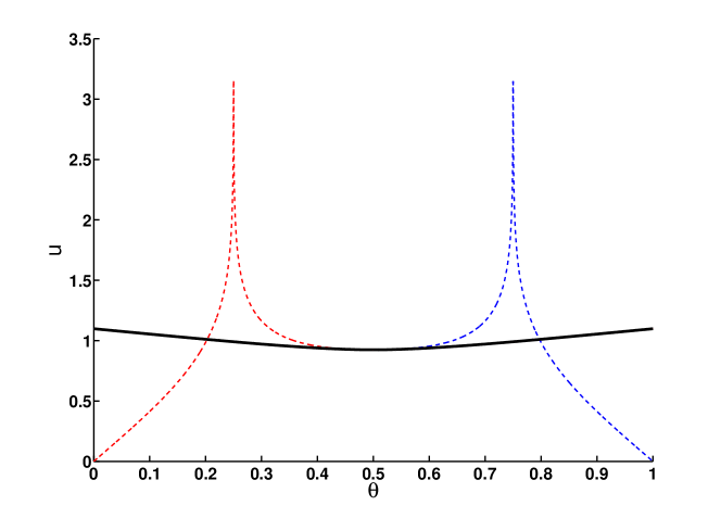
Figure 1: Solution of the Hamilton-Jacobi equation (12) for the critical value $\lambda=\frac{1}{2}$. The two branches (dotted lines, red and blue) correspond to the two possible choices $\alpha=a$, resp. $\alpha=1-a$. The bold line corresponds to the only possible combination of the two branches which gives a bounded viscosity solution.

Let $a\in(0,\frac{1}{2})$. We consider the one-parameter family of matrices

$$\mathcal{M}=\left\{\begin{pmatrix}0&1-\alpha\\ \alpha&0\end{pmatrix}\,,\quad\alpha\in[a,1-a]\right\}\,.$$

The dominant eigenvalue is $\sqrt{\alpha(1-\alpha)}$, with a maximum attained at $\alpha=\frac{1}{2}$. We identify $[0,1]$ and $\mathcal{S}$ under the parameterization

$$\mathcal{S}=\left\{\begin{pmatrix}1-\theta\\ \theta\end{pmatrix}\,,\quad\theta\in[0,1]\right\}\,.$$

We have $L(\theta,\alpha)=\alpha(1-\theta)+(1-\alpha)\theta$, and $b(\theta,\alpha)=\alpha(1-\theta)^{2}-(1-\alpha)\theta^{2}$. We look for a solution $(\lambda,\mathring{u})$ to the Hamilton-Jacobi equation (12). For computing $\mathring{u}$ we have to combine two branches, corresponding to the choice $\alpha=a$ or $\alpha=1-a$. We realize that the first branch has a vertical asymptote at $\theta=z_{a}$ since $b(\cdot,a)$ vanishes at this point, whereas the second branch has a vertical asymptote at $\theta=z_{1-a}$. Therefore there is only one possible combination which gives a bounded viscosity solution on $\mathcal{S}$.

In this example the ergodic set is the segment $[z_{a},z_{1-a}]$.

V Application to the optimization of growth-fragmentation processes in dimension 3

We consider a toy model for a stage-structured linear polymerization-fragmentation process. It is inspired from a nonlinear discrete polymerization-fragmentation introduced in [27] for the dynamics of prion proliferation. We do not take into account nonlinear saturation effects, and we further reduce the size of the system to $n=3$. Polymers can have three states relative to their lengths: small (monomers), medium (oligomers), large (polymers). We denote by $x_{i}$, $i=1,2,3$ the density of polymers in each compartment. Transition rates due to growth in size of polymers from smaller to larger compartments (polymerization) are denoted by $\tau_{i}$, $i=1,2$. Transition rates due to fragmentation from larger to smaller compartments are denoted by $\beta_{i}$, $i=2,3$. The corresponding matrices are

$$\!\!G=\begin{pmatrix}-\tau_{1}&0&0\\ \tau_{1}&-\tau_{2}&0\\ 0&\tau_{2}&0\end{pmatrix}\,\text{and}\,F=\begin{pmatrix}0&2\beta_{2}&\beta_{3}\\ 0&-\beta_{2}&\beta_{3}\\ 0&0&-\beta_{3}\end{pmatrix}\,.$$ (19)

Denoting by $q=(1\;2\;3)^{T}$ the vector of relative sizes of polymers, we have the following properties: $\mathbf{1}^{T}G=0$ (conservation of the number of polymers by growth) and $q^{T}F=0$ (conservation of the total size of polymers by fragmentation).

Optimal control issues come up in the development of efficient diagnosis tools for early detection of prion diseases from blood samples. The protocol PMCA (Protein Misfolding Cyclic Amplification) has been introduced by Soto and co-authors [34, 12] as very powerful method to achieve this goal. It aims at quickly generating in vitro detectable quantities of PrPsc being given minute quantities of it. PMCA consists in successive switching between incubation phases (where aggregates are expected to grow following a seeding-nucleation scenario alimented by purified PrPc) and sonication phases (where breaking of polymers is expected to increase the number of nucleation sites). This clear distinction between two phases with a control parameter which is the intensity of sonication makes the framework of (1) very weel adapted to model PMCA.

The minimal model for PMCA goes as follows: introduce $\alpha:[0,t]\to[a,A]$ the intensity of sonication (i.e. fragmentation). The goal is to maximize the total size of polymers $\left\langle q,x_{\alpha}(t)\right\rangle$ following the linear growth-fragmentation process:

$$\begin{cases}\dot{x}_{\alpha}(s)=(G+\alpha(s)F)x_{\alpha}(s),\\ x_{\alpha}(0)=x\,.\end{cases}$$ (20)

A generalization of this model, which includes an incidence of the sonication on the growth process, is investigated in [16]. For problem (20), corollary 2 implies that $\left\langle q,x_{\alpha}(t)\right\rangle$ has an exponential growth with exponent $\lambda(\mathcal{M})$. When $\tau_{1}=\tau_{2}$ it is clearly better to sonicate as much as possible ($\alpha(s)\equiv A$) because smaller monomers are equally efficient at growing in size than intermediate oligomers, but they are more numerous for a given size. However there are some biological evidence that polymerization rate is size-dependent: polymerization of intermediate aggregates have been postulated to be the most efficient [33] (see also [10] for a continuous PDE model and a discussion of this phenomenon). Mathematically speaking we have a precise description of the variations of $\lambda(\alpha)$ as stated in the following Proposition.

Proposition 13

The Perron eigenvalue $\lambda(\alpha)$ of $G+\alpha F$ reaches a maximum value for some $\alpha^{*}\in(0,+\infty)$ if and only if $\tau_{2}>2\tau_{1}$. Furthermore we face the following alternative:

• either $\tau_{2}\leq 2\tau_{1}$ and $\lambda(\alpha)$ increases from $0$ to $\tau_{1},$

• or $\tau_{2}>2\tau_{1}$ and $\lambda(\alpha)$ increases from $0$ to $\lambda(\alpha^{*})$ and then decreases from $\lambda(\alpha^{*})$ to $\tau_{1}$.

We refer to [9] for the details of the proof of Proposition 13.

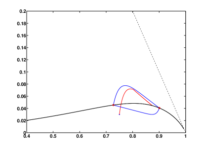
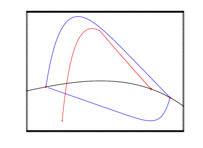
Figure 2: Illustration of convergence of optimal trajectories towards the optimal Perron eigenvector for the three-dimensional growth-fragmentation process (19) with typical parameters. We have plotted the curve of Perron eigenvectors (black line), the boundary of the ergodic set (blue line), and an arbitrary optimal trajectory (red line). The optimal trajectory enters the ergodic set and then converges towards a limit cycle. Right picture is a zoom of the left one. The numerical grid is plotted on the axes: the space step is $\Delta x=5\text{\sc\footnotesize E}{-4}$ to fall much below the width of the ergodic set. Parameters are $\tau_{1}=2\text{\sc\footnotesize E}-2,\tau_{2}=1,\beta=4\text{\sc\footnotesize E}-2$, and $a=2,A=8$.

Qualitative analysis of the optimal control and associated optimal trajectories rely on the description of relevant sets in the simplex. The ergodic set introduced by Arisawa [2, 3] can be characterized as the set enclosed by two remarkable trajectories: each starting from one of the two extremal Perron eigenvectors (resp. $e_{1}(a)$ and $e_{1}(A)$) and evolving with constant control (resp. $A$ and $a$). This set is of particular interest since it attracts all trajectories, not necessarily optimal ones. However it does not give any insight about the fate of optimal trajectories inside the ergodic set.

So far we have only access to local second-order conditions (16) to test the optimality of the best constant control. Numerical tests suggest that we always have $\lambda(\mathcal{M})=\max_{m}\lambda(m)$ in the case of (19), that is to say the optimal trajectory converges towards the optimal Perron eigenvector in the simplex. This is confirmed by finite-volume numerical simulations of the ergodic Hamilton-Jacobi equation (4), see Figure 2. We computed the optimal control $\alpha^{*}$ as a function of the position in the simplex. We observed a clear separation between two connected regions of the simplex (result not shown), corresponding to the extremal choices $\alpha=a$ or $\alpha=A$. This gives an optimal vector field which drives optimal trajectories. Outcomes of the numerical simulations are consistent with the presumable stability of the best constant control against periodic perturbations.

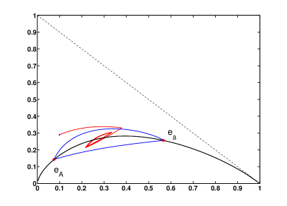
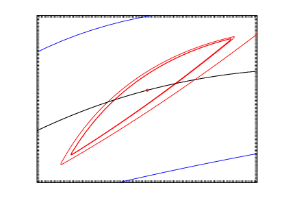
Figure 3: Illustration of the optimal limit cycle for the numerical example (21). We have plotted the curve of Perron eigenvectors (black line), the boundary of the ergodic set (blue line), and an arbitrary optimal trajectory (red line). The optimal trajectory enters the ergodic set and then converges towards a limit cycle. Right picture is a zoom of the left one. The numerical grid is plotted on the axes: the space step is $\Delta x=1\text{\sc\footnotesize E}{-3}$ to fall much below the width of the limit cycle.

A three-dimensional example with an optimal limit cycle

Proposition 9 rules out the existence of optimal limit cycles in dimension $n=2$. Although the previous example of the three-dimensional growth-fragmention process did not exhibit limit cycles apparently, we were able to find another three-dimensional example by testing random choices of matrices with respect to the stability criterion (16):

$$G =\begin{pmatrix}0&0.245&0.007\\ 0&0&0.141\\ 0&0&0\end{pmatrix}$$

$$F =\begin{pmatrix}-0.245&0&0\\ 0.272&-0.499&0\\ 0.645&0.026&-0.035\end{pmatrix}\,.$$ (21)

We assume as in the previous example that the control $\alpha$ takes values in $[a,A]$. The maximal Perron eigenvalue is obtained for $\alpha^{*}\approx 0.415$. The stability criterion (16) has been checked numerically: the optimal constant control is not stable with respect to periodic perturbations at high frequency. Therefore we expect limit cycles to attract optimal trajectories in the simplex in the spirit of the Poincaré-Bendixson theory. This has been checked using finite-volume numerical simulations of the ergodic Hamilton-Jacobi equation (4), see Figure 3. It is worth mentioning that a similar counter-example has been proposed in [18] to answer a question raised in [23]. Our quantitative approach based on second-order conditions provides another example. Furthermore it illustrates the rich possible dynamics of optimal trajectories. The connexion with the Poincaré-Bendixson theory seems appealing. However, proving that limit cycles are the only alternative to pointwise convergence seems out of reach at the moment, due to the complexity of the Poincaré-Bendixson theory in the case of discontinuous vector fields [17].

References

- [1] A. A. Agrachev and Y. L. Sachkov. Control theory from the geometric viewpoint. Springer-Verlag, Berlin, 2004. Control Theory and Optimization, II.
- [2] M. Arisawa. Ergodic problem for the Hamilton-Jacobi-Bellman equation. I. Existence of the ergodic attractor. Annales de l’Institut Henri Poincaré (C) Non Linear Analysis, 14(4):415–438, 1997.
- [3] M. Arisawa. Ergodic problem for the Hamilton-Jacobi-Bellman equation. II. Annales de l’Institut Henri Poincaré (C) Non Linear Analysis, 15(1):1–24, 1998.
- [4] N. E. Barabanov. An absolute characteristic exponent of a class of linear nonstationary systems of differential equations. Sibirsk. Mat. Zh., 29(4):12–22, 222, 1988.
- [5] N. E. Barabanov. On the aizerman problem for third-order time-dependent systems. Diff. Urav., 29(10):1659–1668, 1836, 1993.
- [6] N. E. Barabanov. Asymptotic behavior of extremal solutions and structure of extremal norms of linear differential inclusions of order three. Linear Algebra and its Applications, 428(10):2357–2367, 2008.
- [7] M. Bardi and I. Capuzzo-Dolcetta. Optimal control and viscosity solutions of Hamilton-Jacobi-Bellman equations. Birkhäuser, 1997.
- [8] B. Bonnard, J.-B. Caillau, and E. Trélat. Second order optimality conditions in the smooth case and applications in optimal control. ESAIM Control Optim. Calc. Var., 13(2):207–236 (electronic), 2007.
- [9] V. Calvez and P. Gabriel. Optimal growth for linear processes with affine control. arXiv:1203.5189 [math], Mar. 2012.
- [10] V. Calvez, N. Lenuzza, D. Oelz, J.-P. Deslys, P. Laurent, F. Mouthon, and B. Perthame. Size distribution dependence of prion aggregates infectivity. Math. Biosci., 1:88–99, 2009.
- [11] I. Capuzzo-Dolcetta and P.-L. Lions. Hamilton-Jacobi equations with state constraints. Trans. Amer. Math. Soc., 318(2):643–683, 1990.
- [12] J. Castilla, P. Saà, C. Hetz, and C. Soto. In vitro generation of infectious scrapie prions. Cell, 121(2):195–206, 2005.
- [13] Y. Chitour, P. Mason, and M. Sigalotti. On the marginal instability of linear switched systems. Systems and Control Letters, 61:247–257, 2012.
- [14] J. Clairambault, S. Gaubert, and T. Lepoutre. Comparison of Perron and Floquet eigenvalues in age structured cell division cycle models. Math. Model. Nat. Phenom., 4(3):183–209, 2009.
- [15] J. Clairambault, S. Gaubert, and B. Perthame. An inequality for the Perron and Floquet eigenvalues of monotone differential systems and age structured equations. C. R. Math. Acad. Sci. Paris, 345(10):549–554, 2007.
- [16] J.-M. Coron, P. Gabriel, and P. Shang. Optimization of an amplification protocol for misfolded proteins by using relaxed control. Journal of Mathematical Biology, 2014. DOI: 10.1007/s00285-014-0768-9.
- [17] T. de Carvalho, C. A. Buzzi, and R. D. Euzébio. On Poincaré-Bendixson theorem and non-trivial minimal sets in planar nonsmooth vector fields. arXiv:1307.6825, July 2013.
- [18] L. Fainshil, M. Margaliot, and P. Chigansky. On the stability of positive linear switched systems under arbitrary switching laws. IEEE Transactions on Automatic Control, 54(4):897–899, Apr. 2009.
- [19] A. Fathi. Théorème KAM faible et théorie de Mather sur les systèmes lagrangiens. C. R. Acad. Sci. Paris Sér. I Math., 324(9):1043–1046, 1997.
- [20] A. Fathi. The Weak KAM Theorem in Lagrangian Dynamics. Cambridge Studies in Advanced Mathematics, to appear.
- [21] S. Gaubert and Z. Qu. Dobrushin ergodicity coefficient for markov operators on cones, and beyond, 2013. Eprint arXiv:1302.5226.
- [22] M. Gaye, Y. Chitour, and P. Mason. Properties of barabanov norms and extremal trajectories associated with continuous-time linear switched systems. In Proceedings of the 52nd IEEE Conference on Decision and Control, pages 716–721, Florence, Italie, 2013.
- [23] L. Gurvits, R. Shorten, and O. Mason. On the stability of switched positive linear systems. IEEE Transactions on Automatic Control, 52(6):1099–1103, June 2007.
- [24] V. N. Kolokoltsov and V. P. Maslov. Idempotent analysis and applications. Kluwer Acad. Publisher, 1997.
- [25] B. Lemmens and R. D. Nussbaum. Non-linear Perron-Frobenius theory, volume 189 of Cambridge Tracts in Mathematics. Cambridge University Press, 2012.
- [26] J. Mallet-Paret and R. Nussbaum. Eigenvalues for a class of homogeneous cone maps arising from max-plus operators. Discrete and Continuous Dynamical Systems, 8(3):519–562, July 2002.
- [27] J. Masel, V. Jansen, and M. Nowak. Quantifying the kinetic parameters of prion replication. Biophysical Chemistry, 77(2-3):139–152, 1999.
- [28] O. Mason and F. Wirth. Extremal norms for positive linear inclusions. Linear Algebra and its Applications, 444:100–113, Mar. 2014.
- [29] P. Michel. Optimal proliferation rate in a cell division model. Math. Model. Nat. Phenom., 1(2):23–44, 2006.
- [30] I. D. Morris. Mather sets for sequences of matrices and applications to the study of joint spectral radii. Proc. London Math. Soc., 3(107):121–150, 2013.
- [31] R. D. Nussbaum. Finsler structures for the part metric and Hilbert’s projective metric and applications to ordinary differential equations. Differential Integral Equations, 7(5-6):1649–1707, 1994.
- [32] G.-C. Rota and G. Strang. A note on the joint spectral radius. Nederl. Akad. Wetensch. Proc. Ser. A 63 = Indag. Math., 22:379–381, 1960.
- [33] J. Silveira, G. Raymond, A. Hughson, R. Race, V. Sim, S. Hayes, and B. Caughey. The most infectious prion protein particles. Nature, 437(7056):257–261, Sept. 2005.
- [34] C. Soto, G. P. Saborio, and L. Anderes. Cyclic amplification of protein misfolding: application to prion-related disorders and beyond. Trends in Neurosciences, 25(8):390–394, 2002.
- [35] F. Wirth. The generalized spectral radius and extremal norms. Linear Algebra and its Applications, 342(1–3):17–40, 2002.