Crossover from Equilibration to Aging: (Non-equilibrium) Theory vs. Simulations

Abstract

Understanding glasses and the glass transition requires comprehending the nature of the crossover from the ergodic (or equilibrium) regime, in which the stationary properties of the system have no history dependence, to the mysterious glass transition region, where the measured properties are non-stationary and depend on the protocol of preparation. In this work we use non-equilibrium molecular dynamics simulations to test the main features of the crossover predicted by the molecular version of the recently-developed multicomponent non-equilibrium self-consistent generalized Langevin equation (NE-SCGLE) theory. According to this theory, the glass transition involves the abrupt passage from the ordinary pattern of full equilibration to the aging scenario characteristic of glass-forming liquids. The same theory explains that this abrupt transition will always be observed as a blurred crossover by the unavoidable finiteness of the time window of any experimental observation. We find that within their finite waiting-time window, the simulations confirm the general trends predicted by the theory.

I Introduction

The amorphous solidification of glass- and gel-forming liquids is an ubiquitous non-equilibrium process of enormous relevance in physics, chemistry, biology, and materials science and engineering dawson . In contrast with equilibrium crystalline solids, whose properties have no history dependence, non-equilibrium amorphous solids may exhibit aging and their properties actually depend on their preparation protocol angellreview1 . Although a long and rich theoretical discussion on this subject has lasted already for several decades, building a general and fundamental framework that simultaneously predicts the main universal signatures of these phenomena, as well as their specific features reflecting the particular molecular interactions and the concrete fabrication protocol involved, remains “one of the most relevant challenges of condensed matter” anderson .

Within the last two decades great advances have been made in the field of spin glasses, where a mean-field theory has been developed cugliandolo to describe non-equilibrium states. The models involved, however, cannot describe the evolution of the spatial structure of real angellreview1 or simulated zaccarelli ; hermes ; gabriel structural glass formers. On the other hand, mode coupling theory (MCT) predicts goetze1 ; goetze2 many of the experimentally observed features of the initial slowdown of real and simulated supercooled liquids. As an equilibrium theory, however, it is unable to describe non-equilibrium phenomena such as aging, and predicts a divergence of the $\alpha$-relaxation time $\tau_{\alpha}$ at a critical temperature $T_{c}$, which is never observed in practice angellreview1 ; edigerreview1 ; ngaireview1 .

In recent years, however, a general unifying theory has been developed, which might well provide the long-awaited fundamental framework referred to above. This is the non-equilibrium self-consistent generalized Langevin equation (NE-SCGLE) theory nescgle1 . This theory was built upon a non-stationary extension nescgle1 of Onsager’s general and fundamental laws of linear irreversible thermodynamics and the corresponding stochastic theory of thermal fluctuations onsager1 ; onsager2 ; onsagermachlup1 ; onsagermachlup2 , adequately extended delrio ; faraday to allow for the description of memory effects and spatial non-locality. From this general and abstract formalism, and after a number of theoretical arguments and approximations, the concrete but generic NE-SCGLE theory of irreversible processes in liquids was derived. As summarized below, this theory simultaneously predicts relevant universal signatures of the glass and the gel transitions, as well as specific features reflecting the particular molecular interactions of the systems considered.

For example, for simple liquids with purely repulsive interparticle interactions, the NE-SCGLE theory leads to a simple and intuitive description of the non-stationary and non-equilibrium process of formation of (high-temperature, high-density) hard-sphere–like glasses nescgle3 . For model liquids with repulsive plus attractive interactions, the NE-SCGLE theory predicts a still richer and more complex scenario, which also includes the formation of sponge-like gels and porous glasses by arrested spinodal decomposition nescgle5 at low densities and temperatures. The NE-SCGLE theory has recently been extended to multi-component systems nescgle4 and to systems of non-spherical particles gory1 ; nescgle7 , thus opening the route to the description of more subtle and complex non-equilibrium amorphous states of matter.

Although these predicted scenarios are qualitatively consistent with experimental observations, a more critical and quantitative evaluation is required before this theory can gain acceptance as a reliable microscopic non-equilibrium statistical thermodynamic theory. Thus, the main purpose of the present work is to carry out the first such systematic comparison, using as a reference the results of the molecular dynamics (MD) simulations of Ref. gabriel , which describe the equilibration and aging of a polydisperse hard-sphere (HS) liquid. As it will be shown below, within the time window of the simulations, a remarkable quantitative agreement is observed between the predicted scenario and the simulation results.

This paper is structured as follows: The theoretical arguments and approximations in which the NE-SCGLE theory of irreversible processes is based are briefly summarize in Section II. For simplicity, this summary focuses on the original version of the NE-SCGLE theory which describes the structure and dynamics of monocomponent Brownian liquids. However, in order to model the polydispersity as well as the passage from short-time ballistic to long-time diffusive dynamics involved in the MD simulations, we resort to the molecular version of the recently-developed multicomponent NE-SCGLE theory nescgle4 . To facilitate the reading of this manuscript, however, the discussion of these general theoretical (but rather technical) aspects are collected as Appendices A-D at the end of the manuscript. Thus, Section III contains the main results of this work, which compares the predicted scenario with the simulation results for the crossover from equilibration to aging of a dense polydisperse hard-sphere liquid. Finally, the main conclusions and a discussion of possible directions for further work are contained in Section IV.

II Fundamental basis of the NE-SCGLE theory

As mentioned in the introduction, the non-equilibrium self-consistent generalized Langevin equation (NE-SCGLE) theory was derived as a generic application of the non-equilibrium extension nescgle1 of Onsager’s theory of time-dependent thermal fluctuations. Here we briefly review the main features of this abstract and general formalism, and the manner in which it becomes, in a particular application, a generic theory of the non-equilibrium evolution of the structure and dynamics of simple liquids.

II.1 From a general and abstract formalism to a concrete but generic theory

For Onsager’s theory we mean the general and fundamental laws of linear irreversible thermodynamics and the corresponding stochastic theory of thermal fluctuations, as stated by Onsager onsager1 ; onsager2 and by Onsager and Machlup onsagermachlup1 ; onsagermachlup2 , respectively, and as extended in Refs. delrio ; faraday to allow for the description of memory effects and spatial non-locality. The fundamental assumption of the non-equilibrium extension of Onsager’s theory is that an arbitrary non-equilibrium slow relaxation process may be described as a globally non-stationary, but locally stationary, stochastic process nescgle3 . From this assumption, general time-evolution equation for the non-stationary mean value $\overline{a}_{i}(t_{w})$ and covariance $\sigma_{ij}(t_{w})\equiv\overline{\delta a_{i}(t_{w})\delta a_{j}(t_{w})}$ of the fluctuations $\delta a_{i}(t_{w})=a_{i}(t_{w})-\overline{a}_{i}(t_{w})$ of the $M$ macroscopic state variables $[a_{1}(t_{w}),a_{2}(t_{w}),...,a_{M}(t_{w})]$ are derived.

To apply this canonical formalism one has to define which physical properties are represented by the abstract state variables $a_{i}(t_{w})$. For example, if we have in mind a monocomponent liquid formed by $N$ particles in a volume $V$, we may identify $a_{i}(t_{w})$ with the instantaneous number $N_{i}(t_{w})$ of particles in the volume $\Delta V=V/M$ of the ith cell of an (imaginary) partitioning of the volume $V$ into $M$ cells. Or, better, with the ratio $n_{i}(t_{w})\equiv N_{i}(t_{w})/\Delta V$, which in the limit $\Delta V/V\to 0$ becomes the local particle concentration profile $n(\textbf{r},t_{w})$. As explained in detail in Ref. nescgle1 , this leads to concrete but generic (i.e., applicable to any monocomponent liquid) time evolution equations for the mean value $\overline{n}(\textbf{r},t_{w})$ and for the covariance $\sigma(\textbf{r},\textbf{r}^{\prime};t_{w})\equiv\overline{\delta n(\textbf{r},t_{w})\delta n(\textbf{r}^{\prime},t_{w})}$ of the fluctuation $\delta n(\textbf{r},t_{w})=n(\textbf{r},t_{w})-\overline{n}(\textbf{r},t_{w})$. The first of these equations reads

$$\frac{\partial\overline{n}(\textbf{r},t_{w})}{\partial t_{w}}=D^{0}{\nabla}\cdot b(\textbf{r},t_{w})\overline{n}(\textbf{r},t_{w})\nabla\beta\mu[{\bf r};\overline{n}(t_{w})],$$ (1)

whereas the second is written in terms of the Fourier transform (FT) $\sigma(k;\textbf{r},t_{w})$ of the globally non-uniform but locally homogeneous covariance $\sigma(\textbf{r},\textbf{r}+\textbf{x};t_{w})$,

$$\begin{split}\frac{\partial\sigma(k;\textbf{r},t_{w})}{\partial t_{w}}=&-2k^{2}D^{0}\overline{n}(\textbf{r},t_{w})b(\textbf{r},t_{w})\mathcal{E}(k;\overline{n}(\textbf{r},t_{w}))\sigma(k;\textbf{r},t_{w})\\ &+2k^{2}D^{0}\overline{n}(\textbf{r},t_{w})\ b(\textbf{r},t_{w}),\end{split}$$ (2)

In these equations $D^{0}$ is the particles’ short-time self-diffusion coefficient (apexD0, ), $b(\textbf{r},t_{w})$ is their local reduced mobility, and $\mu[{\bf r};\overline{n}(t_{w})]$ is their chemical potential. $\mathcal{E}(k;\overline{n}(\textbf{r},t_{w}))$ is the FT of $\mathcal{E}[{\bf r},\textbf{r}+\textbf{x};n]\equiv\left[{\delta\beta\mu[{\bf r};n]}/{\delta n(\textbf{r}+\textbf{x})}\right]$.

Eqs. (1) and (2) above correspond to Eqs. (4.1) and (4.3) of Ref. nescgle1 , which discusses other more specific theories and limits that turn out to be contained as particular cases of these equations. For example, let us imagine that we manipulate the system to an arbitrary (generally non-equilibrium) initial state with mean concentration profile $\overline{n}^{0}(\textbf{r})$ and covariance $\sigma^{0}(k;\textbf{r})$, for then letting the system equilibrate for $t_{w}>0$ in the presence of an external field $\psi({\bf r})$ and in contact with a temperature bath of temperature $T$. The solution of Eqs. (1) and (2) then describes how the system relaxes to its final equilibrium state whose mean profile and covariance are $\overline{n}^{eq}(\textbf{r})$ and $\sigma^{eq}(k;\textbf{r})$. Describing this response at the level of the mean local concentration profile $\overline{n}(\textbf{r},t_{w})$ is precisely the aim of dynamic density functional theory (DDFT) tarazona1 ; tarazona2 ; archer , whose central equation is recovered from Eq. (1) in the limit in which we neglect the friction effects embodied in $b(\textbf{r},t_{w})$ by setting $b(\textbf{r},t_{w})=1$ (see Eq. (15) of Ref. tarazona1 ).

The description of the non-equilibrium state of the system in terms of the random variable $n(\textbf{r},t_{w})$ is not complete, however, without the simultaneous description of the relaxation of the covariance $\sigma(k;\textbf{r},t_{w})$ in Eq. (2). In fact, under some circumstances, the main signature of the non-equilibrium evolution of a system may be embodied not in the temporal evolution of the mean value $\overline{n}({\bf r};t_{w})$ but in the evolution of the covariance $\sigma(k;\textbf{r},t_{w})$ (which is essentially a non-uniform and non-equilibrium version of the static structure factor). This may be the case, for example, when a homogeneous system in the absence of external fields remains approximately homogeneous, $\overline{n}({\bf r};t_{w})\approx\overline{n}\equiv N/V$, after a sudden temperature change. Under these conditions, the non-equilibrium process is described only by the solution of Eq. (2). Let us point out that in the limit $b(t_{w})\to 1$ and within the small-wave-vector approximation, $\mathcal{E}(k;\overline{n})\approx\mathcal{E}_{0}+\mathcal{E}_{2}k^{2}$, Eq. (2) becomes the basic kinetic equation describing the early stage of spinodal decomposition (see, for example, Eq. (3.4) of Ref. furukawa ).

Eqs. (1) and (2) above are coupled between them through the local mobility function $b(\textbf{r},t_{w})$, essentially a non-stationary and state-dependent Onsager’s kinetic coefficient. In addition, these two equations are also coupled, through $b(\textbf{r},t_{w})$, with the two-point (van Hove) correlation function $C(\textbf{r},\tau;\textbf{x};t_{w})\equiv\overline{\delta n(\textbf{x},t_{w})\delta n(\textbf{x}+\textbf{r},t_{w}+\tau)}$. According to Ref. nescgle1 , the memory function of $C(\textbf{r},\tau;\textbf{x};t_{w})$ can in its turn be written approximately in terms of $\overline{n}({\bf r};t_{w})$ and $\sigma(k;\textbf{r},t_{w})$, thus introducing strong non-linear effects. Thus, even before solving Eqs. (1) and (2), they reveal a number of relevant features of general and/or universal character.

The most illuminating of them is that, besides the equilibrium stationary solutions $\overline{n}^{eq}(\textbf{r})$ and $\sigma^{eq}(k;\textbf{r})$, defined by the equilibrium conditions $\nabla\beta\mu[{\bf r};\overline{n}^{eq}]=0$ and $\mathcal{E}(k;\overline{n}(\textbf{r},t_{w}))\sigma(k;\textbf{r},t_{w})=1$, Eqs. (1) and (2) also predict the existence of another set of stationary solutions that satisfy the dynamic arrest condition, $\lim_{t_{w}\to\infty}b(\textbf{r},t_{w})=0$. This far less-studied second set of solutions describes, however, important non-equilibrium stationary states of matter, corresponding to common and ubiquitous non-equilibrium amorphous solids, such as glasses and gels.

II.2 Spatial uniformity, a simplifying approximation.

To appreciate the essential physics of this fundamental and universal prediction of Eqs. (1) and (2), the best is to provide explicit examples. To do this without a high mathematical cost, however, let us write $\overline{n}(\textbf{r},t_{w})$ as $\overline{n}(\textbf{r},t_{w})=\overline{n}(t_{w})+\Delta\overline{n}(\textbf{r},t_{w})$, and in a first stage let us neglect the spatial heterogeneities represented by the deviations $\Delta\overline{n}(\textbf{r},t_{w})$. As a result, rather than solving the time-evolution equation for $\overline{n}({\bf r};t_{w})$, we have that $\overline{n}(t_{w})$ now becomes a control parameter, so that we only have to solve the time-evolution equation for the covariance $\sigma(k,\textbf{r};t_{w})$. We may consider, for example, the specific case in which the system is constrained to remain isochoric and spatially homogeneous ($\overline{n}({\bf r};t_{w})\approx\overline{n}\equiv N/V$) after an instantaneous temperature quench at time $t_{w}=0$, from an arbitrary initial temperature to a lower final temperature $T$. For this process, the time-evolution equation for the Fourier transform (FT) $\sigma(k;t_{w})$ of the covariance $\sigma(\textbf{r},\textbf{r}^{\prime};t_{w})=\sigma(\mid\textbf{r}-\textbf{r}^{\prime}\mid;t_{w})$ can be written, for $t_{w}>0$ and in terms of the non-stationary static structure factor $S(k;t_{w})\equiv\sigma(k;t_{w})/\overline{n}$, as

$$\frac{\partial S(k;t_{w})}{\partial t_{w}}=-2k^{2}D^{0}b(t_{w})\overline{n}\mathcal{E}_{f}(k)\left[S(k;t_{w})-1/\overline{n}\mathcal{E}_{f}(k)\right].$$ (3)

in which $\mathcal{E}_{f}(k)=\mathcal{E}(k;\overline{n},T_{f})$ is the Fourier transform (FT) of the functional derivative $\mathcal{E}[\mid\textbf{r}-\textbf{r}^{\prime}\mid;n,T]\equiv\left[{\delta\beta\mu[{\bf r};n]}/{\delta n({\bf r}^{\prime})}\right]$ of the chemical potential $\mu$, evaluated at $n({\bf r})=\overline{n}$ and $T=T_{f}$.

It is important to mention that the solution of this equation yields in principle $S(k;t_{w})$ as output, for given $b(t_{w})$ provided as input. This calls for an independent relationship between these two unknowns, which may have the format of an equation (or system of equations) that accepts $S(k;t_{w})$ as input and yields $b(t_{w})$ as output. This is precisely the role of the following set of equations. The first of them is an expression for the time-evolving mobility $b(t_{w})$,

$$b(t_{w})=[1+\int_{0}^{\infty}d\tau\Delta{\zeta}^{*}(\tau;t_{w})]^{-1},$$ (4)

in terms of the $t_{w}$-evolving, $\tau$-dependent friction coefficient $\Delta{\zeta}^{*}(\tau;t_{w})$, which can be approximated by nescgle1

$$\begin{split}\Delta\zeta^{*}(\tau;t_{w})=\frac{D_{0}}{24\pi^{3}\overline{n}}\int d{\bf k}\ k^{2}\left[\frac{S(k;t_{w})-1}{S(k;t_{w})}\right]^{2}\times\\ F(k,\tau;t_{w})F_{S}(k,\tau;t_{w}).\end{split}$$ (5)

In this equation $\tau$ is the correlation time and $t_{w}$ is the waiting (or evolution) time. $F(k,\tau;t_{w})$ and $F_{S}(k,\tau;t_{w})$ are, respectively, the collective and self non-equilibrium intermediate scattering functions (ISFs), whose respective memory functions are approximated to yield the following approximate expressions for the Laplace transforms (LT) $\hat{F}(k,z;t_{w})$ and $\hat{F}_{S}(k,z;t_{w})$,

$$\hat{F}(k,z;t_{w})=\frac{S(k;t_{w})}{z+\frac{k^{2}D^{0}S^{-1}(k;t_{w})}{1+\lambda(k;t_{w})\ \Delta\hat{\zeta}^{*}(z;t_{w})}},$$ (6)

and

$$\hat{F}_{S}(k,z;t_{w})=\frac{1}{z+\frac{k^{2}D^{0}}{1+\lambda(k;t_{w})\ \Delta\hat{\zeta}^{*}(z;t_{w})}}.$$ (7)

In these equations $\lambda(k)$ is a phenomenological “interpolating function” nescgle1 , given by

$$\lambda(k;t_{w})=1/[1+(k/k_{c}(t_{w}))^{2}],$$ (8)

with $k_{c}(t_{w})$ being an empirically chosen cutoff wave vector.

Eqs. (5)-(8) are the non-equilibrium extension of the corresponding equations of the equilibrium SCGLE theory, which is recovered in the long-$t_{w}$ stationary limit in which $S(k;t_{w}\to\infty)\to S^{(eq)}(k)\equiv 1/\overline{n}\mathcal{E}_{f}(k)$. The derivation of these equations in Ref. nescgle1 also extends to non-equilibrium conditions the same approximations and assumptions employed in the original derivation of the equilibrium SCGLE theory todos2 . Such an extension is quite natural within the framework of the non-equilibrium generalization of Onsager’s theory, but not in the context of the Mori-Zwanzig formalism boonyip , which is deeply rooted in the equilibrium condition.

Coupling Eqs. (3) and (4) with Eqs. (5)-(8) results in the NE-SCGLE closed system of equations that must be solved self-consistently. Thus, the simultaneous solution of Eqs. (3)-(8) above constitutes the NE-SCGLE description of the spontaneous evolution of the structure and dynamics of an instantaneously and homogeneously quenched monocomponent liquid. The only element that we still have to determine is the empirically chosen cutoff wave vector $k_{c}(t_{w})$. For simplicity, we shall define this parameter in reference to the position of the main peak of $S(k;t_{w})$, in an identical manner as the cutoff wave vector $k_{c}^{eq}$ of the equilibrium SCGLE theory is defined in reference to the position of the main peak of $S^{(eq)}(k)$. In this manner, the NE-SCGLE theory becomes a self-consistent theory with no adjustable parameters.

II.3 General physical insights revealed by the NE-SCGLE equations

Being a particular case of Eq. (3), the most relevant and general physical insights provided by Eq. (3) is the NE-SCGLE prediction of the existence of two fundamentally different kinds of stationary solutions, implying the existence of two fundamentally different kinds of states of matter. The first corresponds to ordinary thermodynamic equilibrium states, in which stationarity is attained because the factor $\left[S(k;t_{w})-1/\overline{n}\mathcal{E}_{f}(k)\right]$ on the right side of Eq. (3) vanishes, i.e., because $S(k;t_{w})$ is able to reach its thermodynamic equilibrium value $S^{(eq)}(k;\overline{n},T_{f})=1/\overline{n}\mathcal{E}_{f}(k)$, while the mobility $b(t_{w})$ attains a finite positive long-time limit $b_{f}$.

Under these conditions, one can estimate the equilibration time $t^{eq}_{w}(\overline{n},T_{f})$ of a quench to a final temperature $T_{f}$ at fixed density $\overline{n}$ (or fixed volume fraction $\phi$), as the waiting time such that the difference between $S(k_{max};t_{w})$ and its asymptotic equilibrium value $S^{(eq)}(k_{max};\overline{n},T_{f})$ is sufficiently small, say $[S(k_{max};t_{w})-S_{f}(k_{max})]\approx e^{-5}$. Thus, according to the solution of Eq. (3), the condition defining $t^{eq}_{w}(\phi)$ is $[S(k_{max};t^{eq}_{w})-S_{f}(k_{max})]=\exp[-2k^{2}D_{0}u(t^{eq}_{w})/S_{f}(k_{max})]\approx\exp[-5]$, where $u(t_{w})\equiv\int_{0}^{t_{w}}b(t_{w}^{\prime})dt_{w}^{\prime}$. Since for long waiting times $u(t_{w})\propto b_{f}t_{w}$, later in this paper we shall estimate $t^{eq}_{w}(\phi)$ as

$$t_{w}^{eq}(\overline{n},T_{f})\approx 5S^{(eq)}(k_{max};\overline{n},T_{f})/2k_{max}^{2}D^{0}b_{f},$$ (9)

where $D^{0}b_{f}=D^{(eq)}_{L}(\overline{n},T_{f})$ is the equilibrium long-time self-diffusion coefficient at the final state point $(\overline{n},T_{f})$. This equilibration time is predicted to increase when $b_{f}$ decreases, and to diverges as $1/b_{f}$ when the state point $(\overline{n},T_{f})$ approaches the ergodic–non-ergodic transition line. This means that already in the ergodic neighborhood of this boundary one should experience enormous difficulties in equilibrating the system within practical experimental times.

The second class of stationary solutions of Eq. (3) emerges from the possibility that the long-time asymptotic limit of the kinetic factor $b(t_{w})$ vanishes, so that $dS(k;t_{w})/dt_{w}$ vanishes at long times without requiring the equilibrium condition $\left[S(k;t_{w})-1/\overline{n}\mathcal{E}_{f}(k)\right]=0$ to be fulfilled. Under these conditions $S(k;t_{w})$ will now approach a distinct non-equilibrium stationary limit, denoted by $S_{a}(k)$, which is definitely different from the expected equilibrium value $S_{f}(k)=S^{(eq)}(k;\overline{n},T_{f})$. Furthermore, the difference $[S(k;t_{w})-S_{a}(k)]$ is predicted to decay to zero in an extremely slow fashion, namely, as $t_{w}^{-0.833}$ nescgle3 . This second class of stationary solutions represents dynamically arrested states of matter (glasses, gels, etc.). The properties of these stationary but intrinsically non-equilibrium states, such as $S_{a}(k)$, are predicted to strongly dependent on the preparation protocol (in our example, on $T_{i}$ and $T_{f}$). Furthermore, due to the extremely slow approach to its asymptotic limit, no matter how long we wait, any finite-time measurement will only record the non-stationary, $t_{w}$-dependent value of the measured properties ($S(k;t_{w})$, $F(k,\tau;t_{w})$, $F_{S}(k,\tau;t_{w})$, etc.).

Although the NE-SCGLE system of equations (5)-(8) is highly non-linear, changing variable from $t_{w}$ to $u(t_{w})\equiv\int_{0}^{t_{w}}b(t^{\prime}_{w})dt^{\prime}_{w}$ re-writes Eq. (3) as a linear relaxation equation for $S^{*}(k;u)$,

$$\frac{\partial}{\partial u}\left[S^{*}(k;u)-S_{f}(k)\right]=-\alpha(k)\left[S^{*}(k;u)-S_{f}(k)\right],$$ (10)

with $\alpha(k)\equiv 2k^{2}D^{0}/S_{f}(k)$. The solution of Eq. (3) can thus be written as $S(k;t)=S^{*}(k;u(t))$, with

$$S^{*}(k;u)=S_{f}(k)+\left[S_{i}(k)-S_{f}(k)\right]e^{-\alpha(k)u}.$$ (11)

It also predicts nescgle3 that the non-linearity is actually encapsulated in the time-dependence of the “internal” (or “material”) time $u(t_{w})$, in full consistency with the phenomenological model of aging of Tool and Narayanaswamy tool ; narayanaswamy , commonly used to model aging and to fit a large number of experimental data hornboll ; hecksher ; richert . We thus conclude that the NE-SCGLE theory captures this intriguing and relevant universality and casts it in a more fundamental and precise first-principles physical context.

III Crossover from ergodic equilibration to non-equilibrium aging of a polydisperse hard-sphere liquid

In this section we discuss the quantitative test of a third general insight of the NE-SCGLE theory. This refers to the nature of the high density hard-sphere glass transition. According to the scenario predicted by the NE-SCGLE theory, the discontinuous and singular transition predicted by equilibrium theories (such as MCT or the equilibrium SCGLE theory) for the hard-sphere liquid is intrinsically correct, but essentially unobservable in practice. This is due to the fact that such theories predict the divergence of the equilibrium $\alpha$-relaxation time $\tau^{(eq)}_{\alpha}(\phi)$ at the critical volume fraction $\phi_{a}$ (and that it remains infinite for $\phi\geq\phi_{a}$). Of course, if $\tau^{(eq)}_{\alpha}(\phi)$ becomes infinite, it is reasonable to conjecture that also the equilibration time $t^{(eq)}(\phi)$ (i.e., the time it takes the system to equilibrate after preparation) must also be infinite. If this conjecture were correct, then the predicted diverging equilibrium scenario will not be amenable to experimental tests, due to the unavoidable constraint of any real experiment or measurement, to be limited to finite time-windows.

Let us mention that the previous scenario, in which the control parameter is the volume fraction $\phi$, is also expected to hold almost without change when we consider a sequence of quenches from a common initial temperature $T_{0}$ to a final temperature $T$ along the same isochore. In this case, the control parameter is the temperature $T$, with its inverse $1/T$ playing the role of the volume fraction $\phi$ in the present discussion. This $\phi\leftrightarrow 1/T$ correspondence has been predicted by the equilibrium SCGLE theory (see ref. dtsoft ) and by the present non-equilibrium extension (separate manuscript). It is a fact, however, that in any real experiment (or simulation) one indeed determines a “real” experimental value $\tau_{\alpha}(\phi;t_{w})$ (or $\tau_{\alpha}(1/T;t_{w})$) of the the $\alpha$-relaxation time. In general, however, such measured value $\tau_{\alpha}(t_{w})$ will depend on the waiting time $t_{w}$ after preparation, thus being a non-equilibrium property that cannot be predicted by an equilibrium theory. The power of the NE-SCGLE theory is precisely that it provides a detailed prediction of the non-equilibrium evolution of the system at any finite evolution time $t_{w}$, thus shifting the attention from unobservable infinite-time equilibrium singularities, to the finite-$t_{w}$ non-equilibrium properties actually measured in practice, such as $\tau_{\alpha}(t_{w})$

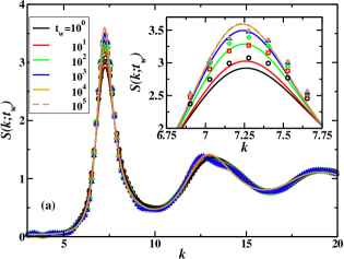
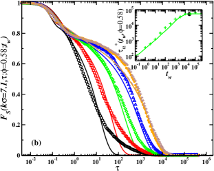
Figure 1: Non-equilibrium evolution of the structure and dynamics of a hard-sphere liquid in the process of its isochoric equilibration at fixed volume fraction $\phi=0{.}58$ according to the (MD) non-equilibrium simulations (symbols) and to the NE-SCGLE theory (solid lines). Fig. 1 Snapshots of $S(k,t_{w})$ as a function of $k$, with a zoom at the main peak in the inset, for the indicated sequence of waiting times. Fig. 1 Corresponding snapshots (from left to right) of $F_{S}(k,\tau;\phi,t_{w})$ plotted as a function of correlation time $\tau$ at fixed $k\sigma=7{.}1$. The inset plots the $\alpha$-relaxation time $\tau_{\alpha}(t_{w},\phi)$, scaled as $\tau_{\alpha}^{*}(t_{w},\phi)\equiv k^{2}D^{0}\tau_{\alpha}(k\sigma;t_{w},\phi)$, as a function of evolution time $t_{w}$, for this equilibration process. The dark asterisk is the equilibration point ($t_{w}^{eq},\tau_{\alpha}^{*eq}$).

These are precisely the predictions that we mean to quantitatively test with the following comparisons. In the particular simulations of Ref. gabriel , a hard-sphere liquid was driven to a non-equilibrium state by means of an effective sudden compression protocol to a final density $\overline{n}$ corresponding to the desired volume fraction $\phi=\pi\overline{n}\sigma^{3}/6$. This protocol is used to generate an ensemble of configurations representative of such non-equilibrium state, characterized by a well-defined initial static structure factor $S_{0}(k;\phi)$. These representative configurations are then taken as the initial condition of an ensemble of standard MD simulation runs describing the non-equilibrium structural relaxation leading to the equilibration (or aging) of the system. This non-equilibrium transient is the subject of study of these simulations (in contrast with ordinary equilibrium simulations, in which this stage is discarded).

The theoretical modeling of the same transient is provided by the simultaneous solution of Eqs. (3)-(8) above, after complementing Eq. (3) with the initial condition $S(k;t=0)=S_{0}(k;\phi)$ and after determining the thermodynamic function $\mathcal{E}_{f}(k)=\mathcal{E}(k;\overline{n},T_{f})$ evaluated at the final state point of the quench. In the present case this corresponds to setting $\overline{n}\mathcal{E}_{f}(k)=\overline{n}\mathcal{E}_{HS}(k;\phi)=1/S^{(eq)}_{HS}(k;\phi)$, for which we use Percus-Yevick’s approximation percusyevick with its Verlet-Weis correction verletweis . For the initial non-equilibrium structure factor $S_{0}(k;\phi)$ we could use directly the result of the simulated non-equilibrium preparation protocol described in the previous paragraph.

Alternatively, we could theoretically model this non-equilibrium structure factor by the equilibrium structure factor of the hard-sphere liquid, $S^{(eq)}_{HS}(k;\phi_{i})$, at an “initial” volume fraction $\phi_{i}$, chosen such that the structural and/or dynamical properties of such equilibrium HS liquid are similar to those of the non-equilibrium state generated by the actual non-equilibrium preparation protocol. In fact, due to dynamical equivalence between soft- and hard-sphere liquids, we could model $S_{0}(k;\phi)$ by the equilibrium static structure factor $S^{(eq)}(k;n_{i},T_{i})$ of any soft-sphere liquid included in the hard-sphere dynamic universality class dtsoft ; atomic3 , provided that the density $n_{i}$ and temperature $T_{i}$ are chosen such that the structural and/or dynamical properties match those of the previously defined hard-sphere liquid, $S^{(eq)}(k;n_{i},T_{i})\approx S^{(eq)}_{HS}(k;\phi_{i})$.

In practice, however, the scenario predicted by the solution of Eqs. (3)-(8) is virtually independent of the specific manner to model the initial non-equilibrium structure factor $S_{0}(k;\phi)$. Thus, in the results that follow, we approximated $S_{0}(k;\phi)$ by the equilibrium static structure factor $S^{(eq)}(k;\phi_{i},T_{i})$ of a polydisperse fluid of soft spheres of diameter $\overline{\sigma}$ and whose interactions are modeled by the Weeks-Chandler-Andersen (WCA) pair potential. In this way, the process start with the system initially at a fluid-like state of temperature $T_{i}=0.06[\epsilon/k_{B}]$ and the same volume fraction $\phi$ of the simulated HS liquid and, at $t_{w}=0$, the temperature is instantaneously lowered to a final value $T_{f}=0$ at which the expected equilibrium state is that of a polydisperse hard-sphere liquid at volume fraction $\phi$.

Fig. 1 illustrates the simplest and most straightforward comparison between the NE-SCGLE theoretical predictions and the simulation results for the non-equilibrium isochoric evolution at fixed $\phi=0.58$ of the HS liquid, in terms of $S(k;t_{w})$ and of the non-equilibrium self intermediate scattering function $F^{S}(k,\tau;t_{w})$ ($\equiv\langle\exp[i\textbf{k}\cdot\Delta\textbf{R}(t_{w})]\rangle$, with $\Delta\textbf{R}(t_{w})=\textbf{R}(t_{w}+\tau)-\textbf{R}(t_{w})$ being the displacement of a tagged particle). This comparison involves a sequence of snapshots of $S(k;t_{w})$ as a function of $k$ (Fig. 1), and of $F^{S}(k=7.1\sigma^{-1},\tau;t_{w})$ as a function of correlation time $\tau$ (Fig. 1), corresponding to a sequence of waiting times $t_{w}=\ 10^{0},\ 10^{1},\ 10^{2},\ 10^{3},\ 10^{4}$ and $10^{5}$ (in molecular time units, $[\sigma\sqrt{M/k_{B}T}]$).

These results illustrate that both, simulations and theory, agree in that no dramatic changes are observed in the evolution of the structure, except for the modest increase in the main peak of $S(k;t_{w})$, zoomed-in in the inset of Fig. 1. In contrast, the dynamics does exhibit a remarkable slowing down, occurring within an “equilibration” time $t_{w}^{eq}(\phi)$. The kinetics of this equilibration process is best summarized by the $t_{w}$-dependence of the non-equilibrium $\alpha$-relaxation time $\tau_{\alpha}(t_{w},\phi)$, defined here by the condition $F_{S}(k=7.1\sigma^{-1},\tau_{\alpha};t_{w},\phi)=1/e$, and illustrated in the inset of Fig. 1 for the equilibration process of the HS liquid at $\phi=0.58$.

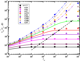
Figure 2: Non-equilibrium Molecular Dynamics simulations (symbols) and NE-SCGLE theoretical results (solid lines for equilibration and dot-dashed lines for aging processes) for the $\alpha$-relaxation time $\tau_{\alpha}^{*}(t_{w},\phi)$, plotted as a function of evolution time $t_{w}$ for a sequence of fixed volume fractions. The asterisks represent the equilibration points $(t^{eq}_{w}(\phi),\tau^{*eq}_{\alpha}(\phi))$ and the dashed line passing through them is the power-law fit $\tau_{\alpha}^{*eq}(\phi)=2.8\times[t_{w}^{eq}(\phi)]^{0.96}$.

At this point let us recall that, in order to prevent crystallization, the MD simulations in the figures actually correspond to an 8.66% (size) polydisperse HS liquid. To properly take this fact into account, the solid lines in Fig. 1 actually correspond to the solution of the NE-SCGLE equations for a polydisperse HS liquid, modeled as an equimolar binary mixture with size ratio yielding a polydispersity of 8.66%. Similarly, to properly compare the NE-SCGLE theoretical predictions (originally derived for Brownian, rather than molecular, liquids) with the present MD simulation data, we applied the long-time dynamic equivalence between Brownian and molecular systems proposed in Ref. AtomicMix , to adapt the NE-SCGLE theory to liquids with underlying molecular microscopic dynamics. This allows us to compare on an equal footing the theoretically-predicted results with the simulated dynamics of the atomic liquid. These methodological aspects of our theoretical calculations are explained in Appendices A-C.

By extending the calculations and comparisons in Fig. 1 to a sequence of other volume fractions in the metastable region of the HS liquid, a more panoramic view emerges of the consistency between the scenarios revealed by theory and by simulations. The results are presented in Fig. 2, which illustrates the extent of the consistency between the main qualitative features of the predicted and the simulated scenarios. For example, in both we see that when the fixed volume fraction is smaller than 0.582, the system will equilibrate within a $\phi$-dependent equilibration time $t_{w}^{eq}(\phi)$ determined by Eq. (9). This equilibration time strongly increases with $\phi$, in a very similar manner as the equilibrium value $\tau_{\alpha}^{eq}(\phi)$ of the $\alpha$-relaxation time. In fact, as can be gathered from the asterisks in the figure, our theory predicts that $t_{w}^{eq}(\phi)\propto[\tau_{\alpha}^{eq}(\phi)]^{\eta}$, with $\eta\approx 1$ (rather than $\eta\approx 1.43$, as determined in the simulations gabriel ; kimsaito ).

For $\phi\geq 0.582$, the NE-SCGLE theory agrees with its equilibrium version (and with MCT) in the prediction that $\tau_{\alpha}^{eq}(\phi)$, and hence also $t_{w}^{eq}(\phi)$, is infinite. This prediction cannot be refuted nor demonstrated, since in practice one can only measure finite $\tau^{*}_{\alpha}(t_{w},\phi)$ at finite waiting times, within finite correlation-time windows. Such finite measurements, however, constitute a stringent and valuable test of the NE-SCGLE theory, which always predicts a finite value for $\tau^{*}_{\alpha}(t_{w},\phi)$ at any finite $t_{w}$. The result of such test is illustrated in Fig. 2 with the four irreversible processes occurring at fixed volume fractions in the non-ergodic regime $\phi\geq 0.582$ (indicated with fill symbols).

For these processes we observe excellent quantitative agreement with the simulation data for $t_{w}\leq 10^{3}$ , but noticeable deviations at longer $t_{w}$. The origin of these deviations might lie in the intrinsic inaccuracies of the approximations involved in the NE-SCGLE theory and/or in the difficulties to simulate the relaxation of a genuine non-ergodic system. For example, for simplicity our theory approximates the mean local density $\overline{n}(\textbf{r};t_{w})$ by its bulk value $n$, thus neglecting structural and dynamical heterogeneities. From the simulation side, the non-equilibrium ensemble employed (see details in the appendix D) involved at least 40 realizations and $1024$ particles. Although this is perfectly adequate for a conventional equilibration process, it is perhaps insufficient at long waiting times in the true non-ergodic regime, as $\phi$ increases far above $\phi_{c}\approx 0.582$.

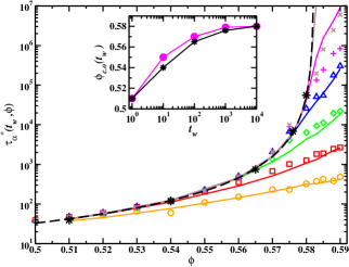
Figure 3: Same as in Fig. 2, but now $\tau_{\alpha}^{*}(t_{w},\phi)$ is plotted as a function of $\phi$ for fixed times $t_{w}=10^{0},\ 10^{1},\ 10^{2},\ 10^{3},$ $10^{4}$ and $10^{5}$ (from bottom to top; the dashed line corresponds to $t_{w}=\infty$). In this case, the dark asterisks indicate the (theoretical) $t_{w}$-dependent volume fraction $\phi_{c.o.}(t_{w})$ that describes the crossover from fully equilibrated to insufficiently equilibrated conditions. In the inset we compare the predicted (asterisks) and simulated (circles) results for $\phi_{c.o.}(t_{w})$.

Although these limitations of the theory and of the simulations must be the subject of more detailed and systematic study, the comparison in Fig. 2 is already highly instructive and revealing, since it provides a kinetic conceptual framework to discuss the nature of the processes of equilibration and aging. To illustrate this, let us now plot the $\alpha$-relaxation time $\tau^{*}_{\alpha}(t_{w},\phi)$ as a function of $\phi$ for a sequence of fixed waiting times. Fig. 3 illustrates that both, theory and simulations, coincide in that the plot of $\tau^{*}_{\alpha}(t_{w},\phi)$ as a function of $\phi$ for a given fixed waiting time $t_{w}$ exhibits two regimes. The first corresponds to samples that have fully equilibrated within this waiting time $(\phi\leq\phi_{c.o.}(t_{w}))$, and the second corresponds to samples for which equilibration is not yet complete $(\phi\geq\phi_{c.o.}(t_{w}))$. The rather loose boundary between these two regimes defines a crossover volume fraction denoted by $\phi_{c.o.}(t_{w})$, illustrated by the asterisks in Fig. 3, which increases with $t$ but seems to saturate to the value $\phi_{c}\equiv\phi_{c.o.}(t_{w}\to\infty)\approx 0.582$ determined by the equilibrium SCGLE theory, as indicated in the inset.

IV Conclusions

In summary, from the theoretical and simulated non-equilibrium results compared in Figs. 1 and 3 we can infer some important conclusions, but also identify several equally relevant issues left open for further discussion. For example, the comparison in Fig. 1 confirms that, at least within the window of waiting times considered, the NE-SCGLE theory captures the correct kinetics of the simulated dynamic arrest transition. This applies particularly to the characteristic feature of the aging of glassy materials observed in the non-equilibrium simulations, namely, the progressive development with waiting time $t_{w}$, of the two-step decay of $F_{S}(k,\tau;t_{w})$ with correlation time $\tau$. Second, the kinetic perspective provided by the non-equilibrium simulations and by the NE-SCGLE theory, defines a useful additional conceptual tool to describe some aspects of the glass transition in model HS liquids. For example, the “equilibrated to non-equilibrated” crossover in the $t_{w}$-dependence of $\tau^{*}_{\alpha}(t_{w},\phi)$ in Fig. 3 could also be interpreted as a “fragile to strong” dynamic crossover that changes with the age of the system fscrossoverchen . This opens the question of the relevance of this NE-SCGLE scenario in the understanding of this actual experimental “fragile to strong” dynamic crossover phenomena observed in many molecular glass-formers fscrossoverchen . This discussion will be facilitated by the NE-SCGLE theory, adapted here to polydisperse or multicomponent atomic liquids, but that must still be extended to thermal protocols involving finite cooling rates.

For the time being, however, the qualitative and quantitative agreement in the comparison in Fig. 2 illustrates the overall consistency between the general scenario observed in the simulations and that predicted by the NE-SCGLE theory. This quantitative test, together with the qualitative consistency with experimental observations of the recently-predicted NE-SCGLE scenario of dynamically arrested spinodal decomposition, provide encouraging evidences of the pertinence and accuracy of this theoretical approach for the description of non-equilibrium dynamic arrest phenomena.

^⋆ Whitacre College of Engineering, Department of Chemical Engineering, Texas Tech University, Lubbock, TX 79409-3121, USA.

^† Shull Wollan Center $-$ Joint Institute for Neutron Sciences, Oak Ridge, TN 37831, USA.

^∗ Departamento de Ingeniería Física, División de Ciencias e Ingenierías, Universidad de Guanajuato, Loma del Bosque 103, 37150 León, México.

Appendix A Multicomponent extension of the NE-SCGLE theory (review of Ref. nescgle4 )

The extension of the NE-SCGLE theory to multicomponent liquid was developed in Ref. nescgle4 . The structural and dynamical properties of a multicomponent liquid are written in terms of the partial static structure factors $S_{\alpha\beta}(k;t_{w})$ and partial (collective and self) intermediate scattering functions, $F_{\alpha\beta}(k,\tau;t_{w})$ and $F^{S}_{\alpha\beta}(k,\tau;t_{w})$, of the binary mixture. The determination of these partial properties involve the solution of the multicomponent version nescgle4 of Eqs. (3)- (8) above.

For an $s$-component mixture, these equations are

$$\frac{\partial S(k;t_{w})}{\partial t_{w}}=-k^{2}D^{0}\cdot b(t_{w})\cdot\Bigl{[}\sqrt{n}\cdot\mathcal{E}(k;n,T_{f})\cdot$$

$$\sqrt{n}\Bigr{]}\cdot S(k;t_{w})-S(k;t_{w})\cdot\Bigl{[}\sqrt{n}\cdot\mathcal{E}(k;n,T_{f})\cdot$$

$$\sqrt{n}\Bigr{]}\cdot b(t_{w})\cdot D^{0}k^{2}+2k^{2}D^{0}\cdot b(t_{w}),$$ (12)

with $\sqrt{n}$ being a $s\times s$ diagonal matrix whose $\alpha$th diagonal element is $\sqrt{n_{\alpha}}$, and in which the element $\mathcal{E}_{\alpha\beta}(k;n,T_{f})$ of the matrix $\mathcal{E}(k;n,T_{f})$ is the Fourier transform (FT) of the functional derivative $\mathcal{E}_{\alpha\beta}[\textbf{r}-\textbf{r}^{\prime};n,T]\equiv\left[{\delta\beta\mu_{\alpha}[{\bf r};n,T]}/{\delta n_{\beta}({\bf r}^{\prime})}\right]\ =\delta({\bf r}-{\bf r}^{\prime})/n_{\alpha}({\bf r})-c_{\alpha\beta}^{(2)}[{\bf r},{\bf r}^{\prime};n,T]$ evaluated at the (fixed) composition $n=(n_{1},...,n_{s})$ and final temperature $T_{f}$ of the quenched system, with $c_{\alpha\beta}^{(2)}[{\bf r},{\bf r}^{\prime};n,T]$ being the direct correlation function. The non-zero elements of the $s\times s$ diagonal matrices $D^{0}$ and $b(t_{w})$ are, respectively, the short-time self-diffusion coefficients $D^{0}_{\alpha}$ and time-dependent mobility functions $b_{\alpha}(t_{w})$, of species $\alpha$. The latter is written as

$$b_{\alpha}[\tau;t_{w}]=\left[1+\int_{0}^{\infty}d\tau\Delta\zeta^{*}_{\alpha}[\tau;t_{w}]\right]^{-1},$$ (13)

with $\Delta\zeta^{*}_{\alpha}[\tau;t_{w}]$ approximated by

$$\Delta\zeta^{*}_{\alpha}(\tau;t_{w})=\frac{D^{0}_{\alpha}}{3\big{(}2\pi\big{)}^{3}}\int d{\bf k}\ k^{2}[F^{S}(\tau)]_{\alpha\alpha}\Bigl{[}h\cdot\sqrt{n}\cdot$$

$$S^{-1}\cdot F(\tau)\cdot S^{-1}\cdot\sqrt{n}\cdot h\Bigr{]}_{\alpha\alpha}.$$ (14)

In this equation the matrix $h$ is given by $h=\sqrt{\overline{n}}^{-1}\cdot(S-I)\cdot\sqrt{\overline{n}}^{-1}$ and we have systematically omitted the arguments $k$ and $t_{w}$ of the $s\times s$ matrices $h(k;t_{w})$, $S(k;t_{w})$, $F(k,\tau;t_{w})$, and $F^{S}(k,\tau;t_{w})$. Finally, the time-evolution equations for $F(k,\tau;t_{w})$ and $F^{S}(k,\tau;t_{w})$ in Laplace space read

$$\hat{F}(k,z;t_{w})=\{zI+k^{2}D^{0}\cdot[zI+$$

$$\lambda(k;t_{w})\cdot\Delta\hat{\zeta}^{*}(z;t_{w})]^{-1}\cdot S^{-1}(k;t_{w})\}^{-1}\cdot S(k;t_{w})$$

and

$$\hat{F^{S}(k,z;t_{w})}=\{zI+k^{2}D^{0}\cdot[zI+$$

$$\lambda(k;t_{w})\cdot\Delta\hat{\zeta}^{*}(z;t_{w})]^{-1}\}^{-1}$$

where $\hat{F}(k,z;t_{w})$ and $\hat{F}^{S}(k,z;t_{w})$ are the Laplace transforms of the collective and self partial intermediate scattering functions $F_{\alpha\beta}(k,\tau;t_{w})$ and $F_{\alpha\beta}^{S}(k,\tau;t_{w})$, and $\lambda(k;t_{w})$ is a diagonal matrix whose non-zero elements $\lambda_{\alpha\alpha}(k;t_{w})$ are given by

$$\lambda_{\alpha\alpha}(k;t_{w})=1/\left[1+\left(k/k^{c}_{\alpha}(t_{w})\right)^{2}\right].$$ (17)

Eqs. (12)- (17) constitutes the essence of the non-equilibrium self-consistent generalized Langevin equation (NE-SCGLE) theory describing the irreversible isochoric relaxation of a suddenly quenched liquid mixture with underlying Brownian or diffusive short-time microscopic dynamics.

Appendix B Molecular adaptation (following Ref. AtomicMix ).

The theoretical predictions presented and discussed in the present paper involve one additional correction, namely, the introduction of a simple interpolating device to incorporate the correct short-time ballistic limit of the dynamics of atomic liquids in the NE-SCGLE dynamic properties (illustrated in Fig. 1). This correction does not affect the essential features of the predicted long-time dynamics associated with the glass transition. However, it is needed to compare the theory, developed for Brownian liquids with underlying short-time diffusive microscopic dynamics, with the results of molecular dynamics simulations, whose short-time dynamics is ballistic. This issue is thus not inherent to the non-equilibrium nature of the NE-SCGLE theory, and in fact, it has recently been discussed in more detail in Ref. AtomicMix in the context of the equilibrium SCGLE theory. In the present work we assume that exactly the same arguments and approximations apply when adapting the NE-SCGLE theory of multicomponent Brownian liquids, summarized in the previous section (Eqs. (12)-(17)), to the description of the dynamics of multicomponent atomic liquids.

In essence, following Ref. AtomicMix , we use the fact that the NE-SCGLE equations (Eqs. (12)-(17)) also describe the non-equilibrium dynamics of the atomic mixture in the long-time diffusive regime, and that a simple manner to interpolate between the correct short-time ballistic and long-time difusive behavior, is provided by the interpolating expressions in Eqs. (4.4)-(4.6) of Ref. AtomicMix . In the present non-equilibrium context, the first of these equations is an integro-diferential equation for the mean square displacement $W_{\alpha}^{(molec)}(\tau;t_{w})$,

$$\frac{M_{\alpha}}{\zeta^{0}_{\alpha}}\frac{dW_{\alpha}^{(molec)}(\tau;t_{w})}{d\tau}+W_{\alpha}^{(molec)}(\tau;t_{w})=D^{0}_{\alpha}\tau-$$

$$\int_{0}^{\tau}\Delta\zeta^{*}_{\alpha}(\tau-\tau^{\prime};t_{w})W_{\alpha}^{(molec)}(\tau^{\prime};t_{w})d\tau^{\prime},$$ (18)

where $M_{\alpha}$ is the mass and $\zeta^{0}_{\alpha}=k_{B}T/D_{\alpha}^{0}$, with $D_{\alpha}^{0}$ being the short-time self-diffusion coefficient of the $\alpha$th atomic species and $T$ being the final temperature of the quench.

The solution of this equation for $W_{\alpha}^{(molec)}(\tau;t_{w})$ satisfies the correct short-time ballistic limit. Introduced in the format of a Gaussian approximation, it guarantees the correct short-time ballistic limit of the collective and self ISFs. To use this fact we follow Eqs. (4.5) and (4.6) of Ref. AtomicMix , which in our non-equilibrium context are written as the following approximate interpolating expressions for the $s\times s$ matrices $F^{(molec)}(k,\tau;t_{w})$ and $F_{S}^{(molec)}(k,\tau;t_{w})$.

$$F^{(molec)}(k,\tau;t_{w})= F(k,\tau;t_{w})+$$

$$\{S(k,t_{w})\cdot\exp[-k^{2}W^{(molec)}(\tau;t_{w})\cdot$$

$$S^{-1}(k,t_{w})]-F(k,\tau;t_{w})\}\cdot\exp[-Z\tau],$$ (19)

and

$$F_{S}^{(molec)}(k,\tau;t_{w})= F_{S}(k,\tau;t_{w})+\{\exp[-k^{2}W^{(molec)}(\tau;t_{w})]$$

$$-F_{S}(k,\tau;t_{w})\}\cdot\exp[-Z\tau].$$ (20)

In these ($s\times s$) matrix equations, the diagonal matrices $W^{(molec)}(\tau;t_{w})$ and $Z$ have diagonal elements $W^{(molec)}_{\alpha}(\tau;t_{w})$ and $Z_{\alpha}\equiv(\zeta^{0}_{\alpha}/M_{\alpha})$, respectively.

The resulting molecular version of the multicomponent NE-SCGLE theory is thus contained in Eqs. (12)-(17) plus Eqs. (18)-(20). The solution of these equations provides a first-principles description of the main dynamic properties of a simple molecular liquid mixture. In a specific application, we start by solving Eqs. (12)-(17) to determine $\Delta\zeta^{*}(\tau;t_{w})$, $F(k,\tau;t_{w})$, and $F_{S}(k,\tau;t_{w})$. These functions describe the short-$\tau$ diffusive dynamics of Brownian, not molecular liquids. To incorporate the correct short-time ballistic limit, we employ these functions as input of Eqs. (18)-(20), thus evaluating $F^{(molec)}(k,\tau;t_{w})$, $F_{S}^{(molec)}(k,\tau;t_{w})$, and $W_{\alpha}^{(molec)}(\tau;t_{w})$. These functions describe the predicted NE-SCGLE dynamics of our atomic or molecular mixture. There, however, we have omitted the superscript $(molec)$, only employed here for the clarity of the present summary.

Appendix C Modeling polydispersity: the atomic hard-sphere liquid.

In order to actually practice the protocol outlined in the last paragraph to solve the NE-SCGLE Eqs. (12)-(20), there are still a few elements that await a more accurate definition. We refer to the short-time self-diffusion coefficients $D_{\alpha}^{0}$, to the cutoff wave-vectors $k^{c}_{\alpha}(t_{w})$ entering in the interpolating functions in Eq. (17), and to the matrix $\mathcal{E}(k;n,T_{f})$. These elements, however, are system-dependent, and hence, must be determined in the context of the concrete model system studied. Thus, let us now address this issue in the context of the monocomponent (but polydisperse) hard-sphere liquid discussed in the paper. This system is modeled in the simulations as a monocomponent but polydisperse hard-sphere liquid with HS diameters subjected to a continuous uniform distribution yielding a polydispersity of 8.66 %.

In the theoretical modeling we approximate this uniform distribution by a binodal distribution yielding the same polydispersity, i.e., as an equimolar binary HS mixture with diameters $\sigma_{1}=(1-\epsilon)$ and $\sigma_{2}=(1+\epsilon)$, with $\epsilon=0.0866$. Hence, the structural and dynamic properties of the resulting bidisperse liquid, $S(k;t_{w})=\sum_{\alpha,\beta=1}^{2}\sqrt{x_{\alpha}x_{\beta}}S_{\alpha\beta}(k;t_{w})$, $F(k,\tau;t_{w})=\sum_{\alpha,\beta=1}^{2}\sqrt{x_{\alpha}x_{\beta}}F_{\alpha\beta}(k,\tau;t_{w})$, and $F_{S}(k,\tau;t_{w})=\ \sum_{\alpha=1}^{2}x_{\alpha}F^{S}_{\alpha}(k,\tau;t_{w})$, are written in terms of the partial static structure factors $S_{\alpha\beta}(k;t_{w})$ and partial (collective and self) intermediate scattering functions, $F_{\alpha\beta}(k,\tau;t_{w})$ and $F^{S}_{\alpha\beta}(k,\tau;t_{w})$ of the binary mixture.

The determination of $D_{\alpha}^{0}$, $k^{c}_{\alpha}(t_{w})$, and $\mathcal{E}(k;n,T_{f})$ must be made at the level of the equilibrium version of the theory. For this we mean the long-$t_{w}$ asymptotic limit of Eqs. (12)-(20) in which the matrix $S(k;t_{w})$ has reached the equilibrium stationary solution of Eq. (12), namely, $S(k;t_{w}\to\infty)\equiv S^{eq}(k;n,T_{f})=\left[\sqrt{n}\cdot\mathcal{E}(k;n,T_{f})\cdot\sqrt{n}\right]^{-1}$. In this limit, Eqs. (14)-(20) become a closed system of equations for the equilibrium dynamic properties $F^{eq}(k,\tau)$, $F_{S}^{eq}(k,\tau)$, and $W_{\alpha}^{eq}(\tau)$, given $S^{eq}(k;n,T)$ as input. This equilibrium theory was developed in Ref. AtomicMix and applied there to the prediction of the equilibrium properties of the same polydisperse hard-sphere liquid discussed in this work. For this, the assumption was made that

$$D^{0}_{1}\approx D^{0}_{2}\approx D^{0}\equiv\frac{3}{8}\left(\frac{k_{B}T}{\pi M}\right)^{1/2}\frac{1}{n\bar{\sigma}^{2}},$$ (21)

and the equilibrium partial static structure factors $S^{eq}_{\alpha\beta}(k)$ were provided by their Percus-Yevick-Verlet-Weis (PYVW) approximation percusyevick ; verletweis , adapted to multicomponent fluids in Ref. williams . Then the cutoff wave-vectors $k^{c}_{\alpha}$ were written as $k^{c}_{\alpha}=1.119k^{max}_{\alpha}$, with $k^{max}_{\alpha}$ being the position of the main peak of $S^{eq}_{\alpha\alpha}(k)$.

Going back to the full non-equilibrium theory employed in this work, in the NE-SCGLE Eqs. (12)-(20), we adopt the same equilibrium definition of $D_{\alpha}^{0}$ in Eq. (21), whereas the matrix $\mathcal{E}(k;n,T_{f})$ needed as input in these equations is determined by the equilibrium condition $\mathcal{E}(k;n,T_{f})=\left[\sqrt{n}\cdot S^{eq}(k;n,T_{f})\cdot\sqrt{n}\right]^{-1}$, with $S^{eq}(k;n,T_{f})$ also approximated by its multicomponent Percus-Yevick-Verlet-Weis (PYVW) approximation percusyevick ; verletweis ; williams . As for the cutoff wave vector $k_{c}(t_{w})$, we also adopt the equilibrium prescription, so that $k_{c}(t_{w})=1.119\times k^{max}_{\alpha}(t_{w})$, with $k^{max}(t_{w})$ being the the position of the main peak of $S(k,t_{w})$.

Appendix D Non-equilibrium molecular dynamics simulations.

In this work we performed non-equilibrium molecular dynamics (NE-MD) simulations to describe the non-equilibrium structural and dynamical evolution of a polydisperse hard-sphere system in their metastable regime close to the glass transition. Our NE-MD simulation data are produced using event-driven simulations and following the same methodology explained in Ref. gabriel . We have used polydisperse samples whose diameters are evenly distributed between $\overline{\sigma}(1-w/2)$ and $\overline{\sigma}(1+w/2)$, with $\overline{\sigma}$ being the mean diameter. In this study, as in the previous work, we have considered the case $w=0.3$, corresponding to a polydispersity $s_{\sigma}=w/\sqrt{12}=0.0866$. The initial configurations are prepared by placing $N$-soft spheres at completely random positions in a cubic cell of volume $V$, interacting through a short ranged repulsive soft (but increasingly harder) interaction and in the presence of strong dissipation, and all the particles are assumed to have the same mass $M$. These nonthermalized hard-sphere configurations are then given random velocities taken from a Maxwell-Boltzmann distribution, with $k_{B}T$ set as the energy unit, and are used as the starting configurations for the event-driven simulations. All results are showed in reduced units, i.e., lenght in units of $\overline{\sigma}$, time in units of $\overline{\sigma}\sqrt{M/k_{B}T}$.

With the purpose of completing our study about the equilibration and aging of a polydisperse hard-sphere (HS) liquid, which is described in Ref. gabriel , we investigate the finite-size effect on the non-equilibrium structural and dynamical evolution of the polydisperse system. We have run simulations over systems of $N$=1024, 2048, 4096 and 8192 spheres and with the intention to generate a reasonable statistical, we have run at least $40$ independent realizations for an array of volume fractions between $0.55$ and $0.58$.

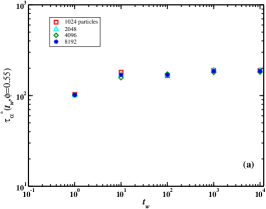
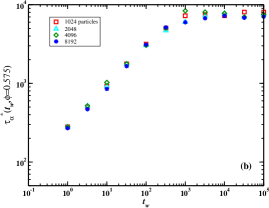
Figure 4: Nonequilibrium evolution of the dimensionless $\alpha$-relaxation time, displayed as $\tau_{\alpha}^{*}(k=7.1;t_{w})$ corresponding to the equilibration processes at fixed volume fractions Fig. 4 $\phi=0.55$ and Fig. 4 $\phi=0.575$.

Our main conclusions are as follow: First, the results obtained do not show a significant dependence on particle number, at least not in all metastable regime, and are independent of the number of realizations. Second, the results are consistent with those reported in Ref. gabriel . This is further illustrated in the Fig. 4 in which we plot the $\alpha$-relaxation time $\tau^{*}_{\alpha}(t_{w},\phi)$, defined by the condition $F_{s}(k,\tau_{\alpha};t_{w})=e^{-1}$, as a function of the evolution time $t_{w}$ for two distinct, representive volume fractions of the metastable regime $\phi$=0.55 and 0.575. As can be noted on the figure, in the case of $\phi=0.55$, the data almost overlap each other for the waiting times considered. In the case of $\phi=0.575$, a slight difference can be observed for higher times than $t_{w}=10^{3}$.

Due to the enormous amount of time required to run the simulation for volume fractions $\phi>0.58$, we have decided not to include the preliminary results here but suggest that the loss of ergodicity becomes a truly fundamental challenge, since the size of the representative non-equilibrium ensemble needed to get stable statistics in the simulations seems to increase without bound as one gets deeper in the glassy regime. This is indeed work in progress, but we believe that the discussion of the paper does exhibit an immediate contribution of the non-equilibrium SCGLE theory, namely, the conceptual enrichment of the discussion of the glass transition problem by introducing the waiting-time dimension $t_{w}$ in the description of glassy behavior.

References

- (1) K. A. Dawson, Current Opinion in Colloid & Interface Science 7, 218 (2002).
- (2) Angell C. A., Ngai K. L., McKenna G. B., McMillan P. F. and Martin S. F., J. Appl. Phys. 88 3113 (2000).
- (3) P. W. Anderson, Science 267 1615 (1995).
- (4) Bouchaud J.-P., Cugliandolo L., Kurchan J., Mezard M., Physica A 226,243 (1996).
- (5) E. Zaccarelli et al., Phys. Rev. Lett. 103, 135704 (2009).
- (6) M. Hermes and M. Dijkstra, J. Phys.: Condens. Matter 22, 104114 (2010).
- (7) G. Pérez, et al., Phys. Rev. E 83, 060501(R) (2011).
- (8) W. Götze, in Liquids, Freezing and Glass Transition, edited by J. P. Hansen, D. Levesque, and J. Zinn-Justin (North-Holland, Amsterdam, 1991).
- (9) W. Götze and L. Sjögren, Rep. Prog. Phys. 55, 241 (1992).
- (10) M. D. Ediger, C. A. Angell, and S. R. Nagel, J. Phys. Chem. 100, 13200 (1996).
- (11) K. L. Ngai, D. Prevosto, S. Capaccioli and C. M. Roland, J. Phys.: Condens. Matter 20, 244125 (2008).
- (12) P. E. Ramírez-González and M. Medina-Noyola, Phys. Rev. E 82, 061503 (2010).
- (13) L. Onsager, Phys. Rev. 37, 405 (1931).
- (14) L. Onsager, Phys. Rev. 38, 2265 (1931).
- (15) L. Onsager and S. Machlup, Phys. Rev. 91, 1505 (1953).
- (16) S. Machlup and L. Onsager, Phys. Rev. 91, 1512 (1953).
- (17) M. Medina-Noyola and J. L. del Río-Correa, Physica 146 A, 483 (1987).
- (18) M. Medina-Noyola, Faraday Discuss. Chem. Soc. 83, 21 (1987).
- (19) L. E. Sánchez-Díaz, P. E. Ramírez-González, and M. Medina-Noyola, Phys. Rev. E 87, 052306 (2013).
- (20) For the definition of in atomic liquids see Appendix C, specifically Eq. (21)
- (21) J. M. Olais-Govea, L. López-Flores, and M. Medina-Noyola, J. Chem Phys. 143, 174505 (2015).
- (22) L. E. Sánchez-Díaz, E. Lázaro-Lázaro, J. M. Olais-Govea and M. Medina-Noyola, J. Chem Phys. 140, 234501 (2014).
- (23) L.F. Elizondo-Aguilera, P. F. Zubieta-Rico, H. Ruíz Estrada, and O. Alarcón-Waess, Phys. Rev. E, 90, 052301 (2014).
- (24) E. Cortés-Morales, L.F. Elizondo-Aguilera, and M. Medina-Noyola, J. Phys. Chem. B, 120 (32), pp 7975-7987 (2016).
- (25) U. Marini Bettolo Marconi and P. Tarazona, J. Chem. Phys. 110, 8032 (1999).
- (26) U. Marini Bettolo Marconi and P. Tarazona, J. Phys.: Condens. Matter 12, A413 (2000).
- (27) A. J. Archer and M. Rauscher, J. Phys. A 37, 9325 (2004).
- (28) H. Furukawa, Adv. Phys., 34, 703 (1985).
- (29) R. Juárez-Maldonado et al., Phys. Rev. E 76, 062502 (2007).
- (30) J. P. Boon and S. Yip, Molecular Hydrodynamics (McGraw-Hill, New York, 1980).
- (31) A. Q. Tool, J. Am. Ceram. Soc. 29, 240 (1946).
- (32) O. S. Narayanaswamy, J. Am. Ceram. Soc. 54, 491 (1971).
- (33) T. Hecksher, N. B. Olsen, K. Niss, and J. C. Dyre, J. Chem. Phys. 133, 174514 (2010).
- (34) R. Richert, Phys. Rev. Lett. 104, 085702 (2010).
- (35) L. Hornboll, T. Knusen, Y. Yue, and X. Guo, Chem. Phys. Lett. 494, 37 (2010).
- (36) J. K. Percus and G. J. Yevick, Phys. Rev. 110, 1 (1957).
- (37) L. Verlet and J.-J. Weis, Phys. Rev. A 5 939 (1972).
- (38) P. E. Ramírez-González, L. López-Flores, H. Acuña-Campa, and M. Medina-Noyola. Phys. Rev. Lett. 107, 155701 (2011)
- (39) L. López-Flores, H. Ruíz-Estrada, M. Chávez-Páez, and M. Medina-Noyola, Phys. Rev. E 88, 042301 (2013).
- (40) E. Lázaro-Lázaro, P. Mendoza-Méndez, L. F. Elizondo-Aguilera, J. A. Perera-Burgos, P. E. Ramírez-González, G. Pérez-Ángel, R. Castañeda-Priego and M. Medina-Noyola, J. Chem Phys. 146, 184506 (2017).
- (41) K. Kim and S. Saito, Phys. Rev. E 79, 060501(R) (2009).
- (42) S H Chen, Y Zhang, M Lagi, S H Chong, P Baglioni and F Mallamace, J. Phys.: Condens. Matter 21, 504102 (2009).
- (43) S. R. Williams and W. van Megen, Phys. Rev. E 64, 041502 (2001).